An Estimate of the Prevalence of BSE in the United States

July 20, 2006

2

EXECUTIVE SUMMARY .......................................................................................................................... 3 INTRODUCTION ........................................................................................................................................ 4 DATA INPUTS FOR THE ANALYSIS ..................................................................................................... 4

COLLECTION PERIOD FOR SAMPLES USED IN THIS ANALYSIS....................................................................... 4 SURVEILLANCE STREAMS ........................................................................................................................... 5 DATA INPUT ASSUMPTIONS........................................................................................................................ 6

MODELING APPROACHES..................................................................................................................... 7 ASSUMPTIONS IN MODELING METHODS ...................................................................................................... 8 ESTIMATION OF PREVALENCE WITH BSURVE PREVALENCE B METHOD ..................................................... 9 ESTIMATION OF PREVALENCE WITH BAYESIAN BIRTH-COHORT METHOD ................................................. 11

SENSITIVITY ANALYSIS ....................................................................................................................... 15 COMPARISON OF THE PREVALENCE ESTIMATE FROM THE BSURVE MODEL TO AN ESTIMATE GENERATED USING A SIMPLER MODEL .......................................................................................................................... 15 SENSITIVITY OF PREVALENCE ESTIMATE TO ADDITIONAL CASES .............................................................. 17 SENSITIVITY OF PREVALENCE ESTIMATE TO ALTERNATIVES FOR ASSUMPTIONS AND INPUT PARAMETERS TO THE BSURVE MODEL. .......................................................................................................................... 18

RESULTS OF PREVALENCE ANALYSIS............................................................................................ 21 RESULTS OF PREVALENCE ANALYSIS ........................................................................................................ 21

RESULTS OF SENSITIVITY ANALYSIS.............................................................................................. 22 SENSITIVITY OF PREVALENCE ESTIMATE TO BSURVE MODEL AND ASSUMPTIONS .................................... 22 SENSITIVITY OF PREVALENCE ESTIMATE TO 1, 2, OR 3 ADDITIONAL POSITIVE ANIMALS ........................... 23 SENSITIVITY OF PREVALENCE ESTIMATE TO ALTERNATIVES FOR ASSUMPTIONS AND INPUT PARAMETERS TO THE BSURVE MODEL. .......................................................................................................................... 24

CONCLUSION OF ANALYSIS ............................................................................................................... 32 APPENDIX A: AGE DISTRIBUTION OF U.S. CATTLE ................................................................... 34

AGE DISTRIBUTION OF THE U.S. NATIONAL HERD..................................................................................... 34 COMPARISON OF NUMBER ENTERING POPULATION TO CULLING AND DEATH LOSSES................................ 36

APPENDIX B. BAYESIAN BIRTH COHORT MODEL (WINBUGS) CODE................................... 38 REFERENCE LIST ................................................................................................................................... 40

3

Executive Summary

The United States has conducted bovine spongiform encephalopathy (BSE) surveillance with increasing intensity since 1990, including an enhanced effort following the identification of a Canadian cow that tested positive in 2003 (APHIS 2006). The goal of this analysis is to estimate the prevalence of BSE in the United States using surveillance data that have been collected over the 7-year period prior to March 17, 2006; this surveillance time frame reflects World Organization for Animal Health (OIE) guidelines, which suggest determining prevalence over a 7-year period. This information will help guide and support future requests for consideration of the overall BSE status of the United States. Moreover, in the interest of transparency, this information will also be made publicly available on the U.S. Department of Agriculture website.

Among the 735,213 cattle sampled in the 7 years prior to March 17, 2006, two infected indigenous animals were identified in addition to the 2003 imported cow from Canada. Results of this analysis suggest that the number of infected cattle in the U.S. is very low.

We estimated the prevalence using two methods. The first estimate is from the BSurvE model (Wilesmith et al., 2004) and is based only on surveillance testing data with no additional information about an effective feed ban. The second method, the Bayesian Birth Cohort model (BBC), was suggested by Vose Consulting in an independent review of the analysis1 and uses the point assignments (sample’s information value) from the BSurvE model. It assumes that the U.S. feed ban implemented in 1997 was at least as effective as a feed ban initiated by the United Kingdom (U.K.) in 1988 and that prevalence in the U.S. would decline proportionately. The mathematical techniques used in this method combine the surrogate U.K. feed ban effectiveness with U.S. surveillance data to provide a more precise estimation of the expected prevalence in the United States.

The most likely value (with upper and lower confidence levels) for the estimated number of BSE infected cattle from the two models was 4 (1,8) (BBC) and 7 (3,24) (BSurvE) in a population of approximately 42 million adult cattle. The results, including upper bounds of both methods, support a conclusion that the prevalence of BSE in the United States is less than 1 infected animal per million adults.

The data were further analyzed to determine the sensitivity of the prevalence estimate to: 1. The BSurvE model and its assumptions, 2. Inclusion of additional cases (for example, the Canadian origin animal) with the

same amount of negative surveillance, and 3. Alternatives for assumptions and input parameters to the BSurvE model.

In each case, the magnitude of change due to the uncertain parameters was not substantial and did not change the conclusion that BSE prevalence is less than 1 infected animal per million adults. The lower and upper bounds from these analyses were 1 to 32 infected animals. When as many as 5 BSE cases (2 indigenous and 3 hypothetical) were included with no additional negatives, the conclusion remained robust with an upper limit of 40. 1 Vose Consulting U.S. LLC, 14 Green Street, Princeton, NJ 08542, USA, www.risk-modelling.com.

4

Introduction

The United States has conducted BSE surveillance with increasing intensity since 1990, including an enhanced effort following the identification of a Canadian cow that tested positive in 2003. This analysis uses surveillance data that have been collected over the 7-year period prior to March 17, 2006, to estimate the prevalence of BSE in the United States. This surveillance timeframe reflects OIE guidelines, which suggest determining prevalence over a 7-year period. The prevalence estimate will help guide and support any future requests for consideration of the overall BSE status of the United States. Prevalence is defined as the proportion of infected animals in a population. Although the simplest approach to the estimation of prevalence is to calculate this proportion directly (e.g., 2 cases / 735,213 samples), the animals sampled for surveillance in the United States were not chosen randomly and represent a population of considerably higher risk than the remaining population. To assess the prevalence, we use two modeling methods for the estimate. The first approach to the estimate uses the BSurvE model developed by the European Union for determining BSE prevalence. The second method uses the BSurvE model’s assignment of point values to each sample and its calculated probability of the animal surviving as input parameters. These parameters are then combined with additional information about an effective feed ban to give a prevalence estimate. The following sections of this document first describe the data used in the analysis and related assumptions inherent in them. Then we present in detail the modeling methods that were used to estimate the prevalence and assumptions for model parameters. Next, we investigate the effect of uncertain parameters and assumptions that have the largest impact on the estimate. We present the results of the prevalence analysis and the sensitivity of the estimate to the uncertain parameters and finally, close with a summary and conclusion of the analysis. Data inputs for the analysis

Collection period for samples used in this analysis Consistent with OIE guidelines for BSE surveillance, this analysis used surveillance data collected over a 7-year period from April 1, 1999, through March 17, 2006, taking into account the long incubation period for BSE. Table 1 summarizes the 7-year totals of surveillance testing and numbers of cattle in each surveillance stream.

5

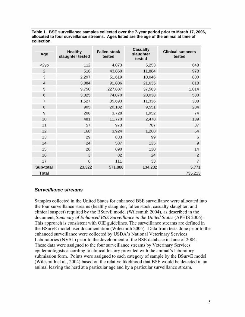
Table 1. BSE surveillance samples collected over the 7-year period prior to March 17, 2006, allocated to four surveillance streams. Ages listed are the age of the animal at time of collection.

Age Healthy slaughter tested

Fallen stock tested

Casualty slaughter

tested Clinical suspects

tested

<2yo 112 4,073 5,253 648 2 518 43,860 11,884 978 3 2,297 51,619 10,046 800 4 3,884 91,806 21,635 818 5 9,750 227,887 37,583 1,014 6 3,325 74,070 20,038 580 7 1,527 35,693 11,336 308 8 905 20,182 9,551 284 9 208 3,728 1,952 74

10 481 11,770 2,478 139 11 57 973 787 37 12 168 3,924 1,268 54 13 29 833 99 6 14 24 587 135 9 15 28 690 130 14 16 3 82 24 2 17 6 111 33 7

Sub-total 23,322 571,888 134,232 5,771Total 735,213

Surveillance streams Samples collected in the United States for enhanced BSE surveillance were allocated into the four surveillance streams (healthy slaughter, fallen stock, casualty slaughter, and clinical suspect) required by the BSurvE model (Wilesmith 2004), as described in the document, Summary of Enhanced BSE Surveillance in the United States (APHIS 2006). This approach is consistent with OIE guidelines. The surveillance streams are defined in the BSurvE model user documentation (Wilesmith 2005). Data from tests done prior to the enhanced surveillance were collected by USDA’s National Veterinary Services Laboratories (NVSL) prior to the development of the BSE database in June of 2004. These data were assigned to the four surveillance streams by Veterinary Services epidemiologists according to clinical history provided with the animal’s laboratory submission form. Points were assigned to each category of sample by the BSurvE model (Wilesmith et al., 2004) based on the relative likelihood that BSE would be detected in an animal leaving the herd at a particular age and by a particular surveillance stream.

6

Data Input Assumptions

Likelihood ratio. Recorded clinical signs for many animals tested during the enhanced surveillance were compatible with BSE but these animals were not initially assigned to the clinical suspect category. For the summary analysis of enhanced surveillance, these animals were assigned to the clinical suspect category if they exhibited signs that were at least 807 times more likely to be found in BSE cases than the U.S. targeted population (APHIS 2006). The denominator of the ratio (likelihood of signs in cases / likelihood of signs in non-cases) is assumed to include all of the negative surveillance data from enhanced surveillance including animals submitted with minimal clinical history. We assume that the 807 threshold and the denominator value correctly capture animals that appropriately should be considered as clinical suspects by BSurvE. The sensitivity of the prevalence estimate to this assumption is discussed in the sensitivity analysis section.

Model parameters affected by population age distribution.

o Exit probability for uninfected animals (Dt) at time t (BSurvE Model Table 6) are derived from the age distribution of the healthy cattle population. Calculations in the BSurvE model assume that a specific number of calves are born each year and that the birth cohort size will decrease across time. It also assumes that the population dynamics are stable from year to year. The model requires an idealized “average” distribution to describe the population. Because the exact age distribution of the 42 million U.S. adult cattle is unknown, a careful estimation of an idealized age distribution is presented in Appendix A. (The sensitivity of the prevalence estimate to this assumption is discussed in the sensitivity analysis section.).

o Exit probabilities for infected animals (Ct). Data to determine the distribution of exiting infected animals (BSurvE model Table 3) are dependent on the incubation period of the disease. These data are not available for the United States because there have been very few cases. Values included in the BSurvE model were based on U.K. experience with the disease and are assumed reasonable for the U.S.. The sensitivity of the prevalence estimate to this assumption is discussed in the sensitivity section.

o Proportion of uninfected and infected cattle that will exit via each surveillance stream (dj|t and cj|t). These data (BSurvE model Table 4 and 5) are not available for the United States; however, the data included in the downloaded BSurvE model were deemed by USDA Veterinary Services epidemiologists to be a reasonable approximation for the United States. The sensitivity of the prevalence estimate to this assumption is discussed in the sensitivity section.

7

Modeling Approaches

U.S. surveillance data presented in this report include 735,213 tests over the 7-year period with two positive indigenous animals and one imported animal. A very simple crude estimate of prevalence is the quotient of 2 / 735,213 or 3 / 735,213 (i.e., 2.7 or 4.0 cases per million high-risk cattle respectively). However, the sampling methodology used to collect the samples was intentionally biased to select from a population of cattle targeted to have high risk of demonstrating BSE (i.e., adult cattle showing clinical signs involving the central nervous system and dead and nonambulatory cattle with clinical signs that could not be evaluated). Medical knowledge of the clinical presentation of BSE suggests that these animals are many times more likely than the general population of cattle to present with BSE (e.g., European data on a similar population suggests that they are 28 times more likely to present with BSE) (EFSA, 2004). However, this crude estimate of prevalence considers only detectable infected cattle, which likely represents only about 40 percent of BSE cases (Wilesmith et al., 2004)2. Using these approximations, the prevalence estimate would be less than 1 BSE infected animal per million adult cattle. Other methods of estimation have been developed that more precisely account for population differences and demographics. A recently developed model, which was designed to utilize cattle demographics, rate of exit from the populations, and known disease characteristics, is the BSurvE model (Wilesmith et al., 2004). This model directly estimates likelihood of finding BSE and assigns a point value to each surveillance sample compared to the information that might be gained from a random sample. Because BSurvE was designed for analysis of BSE targeted surveillance and has received favorable international review (EFSA, 2004), it was chosen as a method for prevalence analysis in the United States. Although BSurvE estimates prevalence in the standing cattle population from surveillance data, it does not incorporate further information about the presence or efficacy of a feed ban. For example, given knowledge of an effective feed ban yet no surveillance data, one might arrive at informed conclusions about the prevalence at some future time (e.g., the Harvard-Tuskegee model predicts a decline to near zero within a few years) (Cohen et al., 2001, 2003). The addition of a small bit of surveillance data would support or detract from that assessment while a large enough amount of data would eventually overwhelm any assumptions regarding feed-ban effects. Bayesian methods of analysis allow mathematical inclusion of the surveillance data and prior knowledge about prevalence to give a final estimate reflecting the total of available information. Because of its ability to incorporate all data, this method of analysis was also conducted to determine BSE prevalence. 2 To further test Wilesmith’s assumption that 40% of BSE cases survive long enough to become detectable, we calculate that 39.97 percent of BSE infected survive long enough to become detectable. This calculation is based on data, time specific exit probabilities, and incubation algorithm from the Harvard-Tuskegee BSE risk model (Cohen et al. 2003) and assumes that animals become infected at 6 months.

8

Assumptions in modeling methods Statistical models of disease are designed to provide a mathematical description of real world events that affect populations. Clearly, in a perfect world where absolute knowledge was possible, prevalence would simply be the number of known-infected animals in the sample divided by the number of samples collected. However, because exact information is often not possible, models must use reliable estimates, averages, or probability distributions to capture values from statistically large numbers to draw conclusions. The following assumptions are inherent in the mechanics of the analytic models described. Where indicated, a quantitative treatment of their impacts is provided in the sensitivity analysis section of this document.

Proportion of pre-clinical detection. The current version of BSurvE allows variation in the percentage of animals detectable in the pre-clinical phase of infection. In this analysis, the proportion of animals that would be detectable if they left the herd in the year prior to showing clinical signs was defined as 40 percent. The sensitivity of the prevalence estimate to this assumption is discussed in the sensitivity section.

Infection in first year of life. BSurvE and BBC assume that all animals are infected in the first year of life. Since the likelihood of infection after the first year is small, the effect of its bias on the outcome of the model is minimized (Wilesmith et al., 2004).

Constant versus declining prevalence. BSurvE Prevalence B assumes a constant incidence of new cases through all years while the Bayesian Birth Cohort (BBC) method diverges from BSurvE and assumes that incidence was constant prior to the feed ban but began to decline afterward. Although both assumptions cannot be correct, the outcomes of the two analyses are essentially equal and indicate that the assumption has negligible influence on the models (see results).

The U.S. feed ban is at least as effective as the 1988 U.K. ban. BSE prevalence in the U.K. declined rapidly for each birth cohort born after the U.K. implemented the 1988 feed ban. For the BBC model, we assume that the U.S. mammalian-to-ruminant feed ban of 1997 was as effective as the U.K. ruminant-to-ruminant ban in 1988 and that prevalence will decline proportionally. The BSurvE model does not include data about the feed ban. (This assumption is discussed in detail in the BBC model section.)

Sensitivity of testing clinical animals. BSurvE assumes infected animals tested more than a year before they develop clinical signs are non-detectable (i.e., sensitivity equals 0 percent). BSurvE also assumes the sensitivity of testing is 100 percent if the animal has reached a stage of infection showing clinical signs (Wilesmith et al., 2004). Nevertheless, BSurvE assumes that animals tested within one year of when they would show clinical signs are only detectable in this preclinical phase 40 percent of the time.

Disease behavior. The BSurvE analysis and the BBC method assume that the biological characteristics of BSE, such as incubation time, clinical presentation, age of infection, and age related exit probability of infected animals, are primarily dependent on the biology of the disease rather than the country in which they occur.

9

Although population demographics and management practices may vary, it is unlikely that the disease would behave differently in different countries. To further assess this assumption, the sensitivity of prevalence to the latency period (Cj,t) in the BSurvE model parameters) of BSE is evaluated in the sensitivity analysis section.

Influence of sampling. The BSE surveillance data represent a very large, targeted sample covering all cattle producing regions in the country. The BSurvE model requires only independence between observations and not random selection of samples (Wilesmith, et al., 2004). However, its authors suggest “…it is important to include the requirement that a country-wide geographic coverage be included, without being too prescriptive” (Wilesmith et al., 2004). Because the sampling strategy for BSE surveillance collected samples from all parts of the United States, we assume that it satisfies the requirements of the BSurvE model. for further detail on sample coverage (See Summary of Enhanced BSE Surveillance) (APHIS 2006).

Prior distribution for BBC. The BBC method assumes that prior to collection of surveillance data, BSE prevalence could have been any value from zero to 100 percent of the cattle in the United States. Although this prior distribution assumes no knowledge about prevalence, it is completely overwhelmed by data and minimally influences the outcome of the model (see results).

Estimation of prevalence with BSurvE Prevalence B method BSurvE Version 06.03 was downloaded March 22, 2006, from http://www.bsurve.com. The BSurvE Web site includes the current version of the BSurvE model as well as documentation that provides detailed descriptions of the underlying functions of the model and step-by-step user instructions (Wilesmith et al., 2005; Wilesmith et al., 2004). The following paragraphs describe the model and provide an overview of the more detailed information provided by the BSurvE supporting documentation. The BSurvE model is designed to estimate prevalence of BSE in a national cattle herd based on targeted sampling strategies similar to U.S. surveillance. Since it was designed to estimate prevalence of BSE and has received positive review (EFSA, 2004), it was chosen as a method to estimate the prevalence of BSE in the U.S. adult cattle population as of March 17, 2006. The BSurvE model uses epidemiologic information accumulated during the U.K. and European outbreaks to predict parameters such as the incubation period of BSE, probable length of an infected animal’s life, and the dynamics of disease expression in infected animals. It combines this information with the surveillance test data to assign point values for targeted samples taken from different surveillance streams. The points represented by an animal tested for BSE are based on the relative likelihood that the disease would be detected in an animal leaving the herd at a particular age and by a particular surveillance stream. Under this scheme, one point is equivalent to a test from an animal randomly selected for testing from the national herd (Wilesmith et al., 2004).

10

The BSurvE model provides two separate estimation methods that differ in purpose. The first method, referred to as the Prevalence A method, is relevant in a country with endemic infection because its prime objective is to determine whether the infection rate is decreasing because of control measures. This method treats each birth cohort independently to enable evaluation of differences in BSE prevalence from year to year among birth cohorts. It also estimates prevalence in the current population of adult cattle by adding the estimated number of infected cattle from each birth cohort that remain alive until the present. The second BSurvE prevalence estimation method, referred to as the Prevalence B method, is intended for use in non-endemic countries. These are defined as countries where “either no cases have been detected despite a continuing surveillance program, or a very small number of cases have been detected, insufficient to indicate that the BSE agent has been distributed in the country to a significant degree” (Wilesmith et al., 2004, p. 7). This method assumes there is a period of time across which the infection rate in a country remains reasonably constant and estimates prevalence across all surveillance data accumulated during that time. We decided, based on our analysis and feedback from the BSurvE authors, that the Prevalence B method was the more appropriate of the two methods for the U.S. Therefore, results from this estimation method are reported here. The BSurvE model is noteworthy for its sound epidemiologic structure, including stratifying cattle by age and cause of death (healthy slaughter, fallen stock, casualty slaughter, or clinical suspect) and accounting for the relative likelihood of detecting BSE in various strata (EFSA, 2004). However, the EFSA review indicates that numerous country-specific BSurvE inputs (e.g., exit constants for uninfected cattle, exit constants for infected animals, proportion of infected or uninfected cattle that would exit in each surveillance stream) often must be based on expert opinion and may lack precision due to the variation of individual opinions (EFSA, 2004). BSurvE serves to interpret BSE surveillance information characterized by age of cattle sampled and surveillance stream. The four surveillance streams (healthy slaughter, fallen stock, casualty slaughter, and clinical suspect) differ with respect to the point values that samples from each stream contribute to the total U.S. surveillance system (APHIS 2006).3 For any combination of cattle age and surveillance stream, the number of points allotted to a sample is calculated by BSurvE. These points are accumulated across all samples to determine prevalence given the number of positive samples observed. A 90 percent confidence interval for prevalence is also computed; it is bounded by the 5th and 95th percentiles of the prevalence uncertainty distribution. The point value concept was developed to account for targeted sampling. Higher point values are assigned to samples with a higher likelihood of being positive. The BSurvE methods are based on this concept, which was published by Cannon in a manuscript on combining surveillance data from multiple sources (Cannon 2002). These methods are further enhanced to weight samples by the likelihood that the sample tests positive. 3 Allocation of animals to surveillance streams is described in detail in the document Summary of Enhanced BSE Surveillance.

11

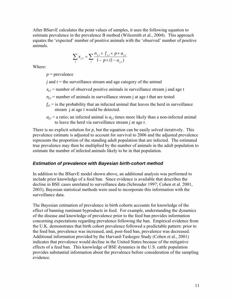
After BSurvE calculates the point values of samples, it uses the following equation to estimate prevalence in the prevalence B method (Wilesmith et al., 2004). This approach equates the ‘expected’ number of positive animals with the ‘observed’ number of positive animals.

∑∑ −×−×××

=j tj

tjtjtj

jtj ap

apfnx

)1(1 ,

,,,,

Where:

p = prevalence

j and t = the surveillance stream and age category of the animal

xj,t = number of observed positive animals in surveillance stream j and age t

nj,t = number of animals in surveillance stream j at age t that are tested

fj,t = is the probability that an infected animal that leaves the herd in surveillance stream j at age t would be detected.

aj,t = a ratio; an infected animal is aj,t times more likely than a non-infected animal to leave the herd via surveillance stream j at age t.

There is no explicit solution for p, but the equation can be easily solved iteratively. This prevalence estimate is adjusted to account for survival to 2006 and the adjusted prevalence represents the proportion of the standing adult population that are infected. The estimated true prevalence may then be multiplied by the number of animals in the adult population to estimate the number of infected animals likely to be in that population.

Estimation of prevalence with Bayesian birth-cohort method In addition to the BSurvE model shown above, an additional analysis was performed to include prior knowledge of a feed ban. Since evidence is available that describes the decline in BSE cases unrelated to surveillance data (Schreuder 1997; Cohen et al. 2001, 2003), Bayesian statistical methods were used to incorporate this information with the surveillance data. The Bayesian estimation of prevalence in birth cohorts accounts for knowledge of the effect of banning ruminant byproducts in feed. For example, understanding the dynamics of the disease and knowledge of prevalence prior to the feed ban provides information concerning expectations regarding prevalence following the ban. Empirical evidence from the U.K. demonstrates that birth cohort prevalence followed a predictable pattern: prior to the feed ban, prevalence was increased, and, post-feed ban, prevalence was decreased. Additional information provided by the Harvard-Tuskegee Study (Cohen et al., 2001) indicates that prevalence would decline in the United States because of the mitigative effects of a feed ban. This knowledge of BSE dynamics in the U.S. cattle population provides substantial information about the prevalence before consideration of the sampling evidence.

12

The Prevalence B method described above assumes that the prevalence of BSE is constant across all birth cohorts. This assumption is questionable from an epidemiological perspective because the feed ban serves to break any established cycle of infection. Thus, prevalence is expected to decrease in each successive birth cohort after the feed ban was established in 1997. The Bayesian Birth Cohort method provides a more precise estimate of U.S. prevalence by combining the epidemiology underlying the BSurvE model with information about the effect of the feed ban on prevalence. This method assumes a priori that prevalence could be any fractional value between 0 and 1, then uses the total surveillance point values for each birth cohort sampled in the United States to inform the prevalence estimate. These point values were determined using the BSurvE model and are displayed in Table 2. Table 2. Point values calculated by BSurvE for each birth cohort are shown below. The column on the right lists the birth cohorts in which positive animals were found.

Age cohort Total point value Number positive 2004 17,057 0 2003 81,573 0

2002 281,496 0 2001 810,504 0

2000 1,563,402 0 1999 1,482,719 0

1998 1,062,070 0 1997 923,217 0

1996 346,751 1 1995 115,128 0

1994 52,263 0 1993 8,830 1

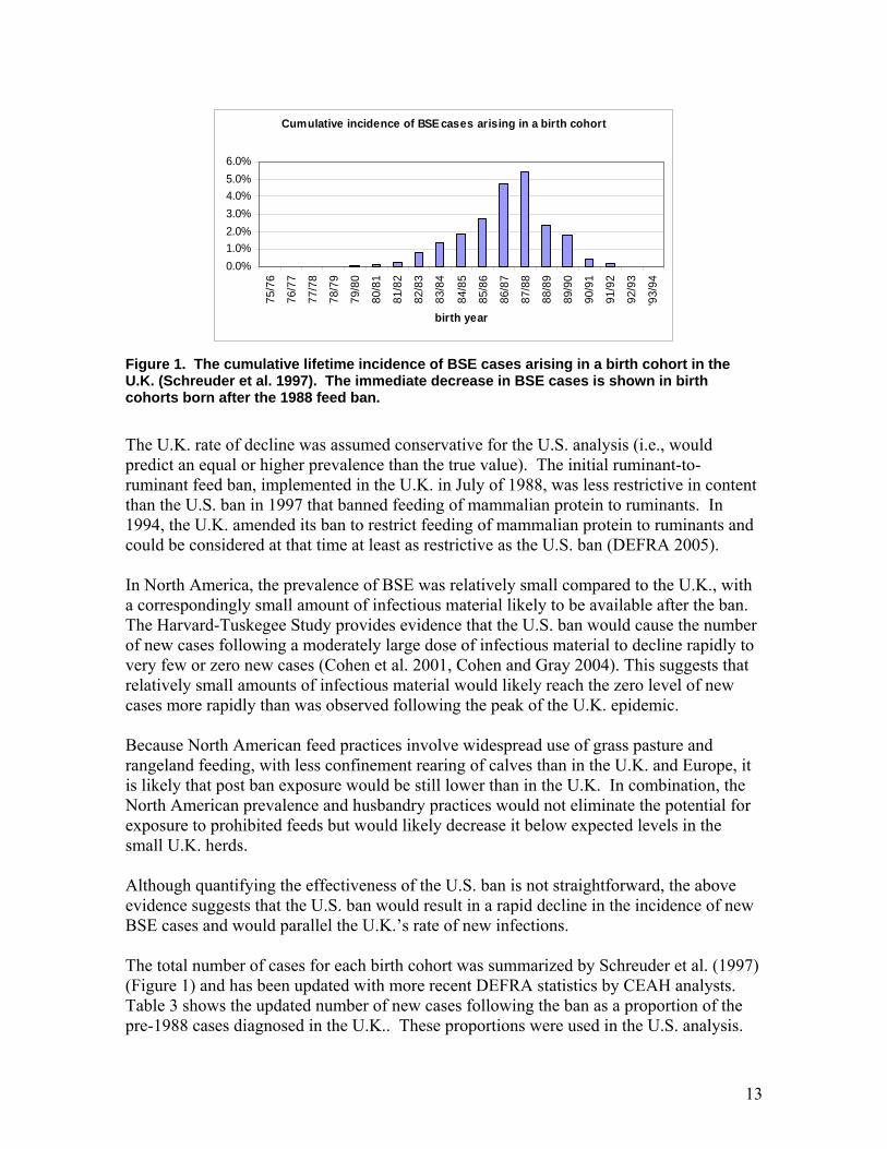
Prevalence in each birth cohort was assumed constant until the effect of the 1997 feed ban rule. From that point forward, the number of new infections each year would be expected to decrease. Because only two cases of BSE were detected in the United States, insufficient data exists to estimate the effect of the feed ban on prevalence in each birth cohort. To address this shortcoming, the reduction in prevalence in each birth cohort was assumed equivalent to the reduction in prevalence observed in the U.K.. This evidence was used to adjust the estimated prevalence for birth cohorts born in 1998 or later in the model. There is little argument that the implementation of feed mitigations will decrease the risk of new BSE cases. Note in the epidemic curve shown in Figure 1 that although the U.K.’s BSE epidemic was on the upswing when the 1988 ban was implemented, it declined rapidly for each cohort of cattle born after the ban. The rate of decline is easily quantifiable from data that are available from the U.K. epidemic before and following the 1988 ruminant-to-ruminant feed ban (DEFRA statistics, 2005).

13

Cumulative incidence of BSE cases arising in a birth cohort

0.0%1.0%2.0%3.0%4.0%5.0%6.0%

75/7

6

76/7

7

77/7

8

78/7

9

79/8

0

80/8

1

81/8

2

82/8

3

83/8

4

84/8

5

85/8

6

86/8

7

87/8

8

88/8

9

89/9

0

90/9

1

91/9

2

92/9

3

'93/

94

birth year

Figure 1. The cumulative lifetime incidence of BSE cases arising in a birth cohort in the U.K. (Schreuder et al. 1997). The immediate decrease in BSE cases is shown in birth cohorts born after the 1988 feed ban.

The U.K. rate of decline was assumed conservative for the U.S. analysis (i.e., would predict an equal or higher prevalence than the true value). The initial ruminant-to-ruminant feed ban, implemented in the U.K. in July of 1988, was less restrictive in content than the U.S. ban in 1997 that banned feeding of mammalian protein to ruminants. In 1994, the U.K. amended its ban to restrict feeding of mammalian protein to ruminants and could be considered at that time at least as restrictive as the U.S. ban (DEFRA 2005). In North America, the prevalence of BSE was relatively small compared to the U.K., with a correspondingly small amount of infectious material likely to be available after the ban. The Harvard-Tuskegee Study provides evidence that the U.S. ban would cause the number of new cases following a moderately large dose of infectious material to decline rapidly to very few or zero new cases (Cohen et al. 2001, Cohen and Gray 2004). This suggests that relatively small amounts of infectious material would likely reach the zero level of new cases more rapidly than was observed following the peak of the U.K. epidemic. Because North American feed practices involve widespread use of grass pasture and rangeland feeding, with less confinement rearing of calves than in the U.K. and Europe, it is likely that post ban exposure would be still lower than in the U.K. In combination, the North American prevalence and husbandry practices would not eliminate the potential for exposure to prohibited feeds but would likely decrease it below expected levels in the small U.K. herds. Although quantifying the effectiveness of the U.S. ban is not straightforward, the above evidence suggests that the U.S. ban would result in a rapid decline in the incidence of new BSE cases and would parallel the U.K.’s rate of new infections. The total number of cases for each birth cohort was summarized by Schreuder et al. (1997) (Figure 1) and has been updated with more recent DEFRA statistics by CEAH analysts. Table 3 shows the updated number of new cases following the ban as a proportion of the pre-1988 cases diagnosed in the U.K.. These proportions were used in the U.S. analysis.

14

Table 3. Number of BSE cases in the U.K. by cohort and proportion of cases in cohorts born after the feed ban relative to number of cases in the last cohort born before the ban

Years since feed ban

U.K. Birth

cohort

BSE cases in the U.K.

Proportion of the

1987/88 U.K.

cohort’s incidence

U.S. Birth

cohort

Years since feed ban

0 1987/88 39,201 1.0 1997 0 1 1988/89 16,556 0.42 1998 1 2 1989/90 11,044 0.28 1999 2 3 1990/91 5,036 0.128 2000 3 4 1991/92 4,348 0.11 2001 4 5 1992/93 3,231 0.08 2002 5 6 1993/94 2,517 0.06 2003 6 7 1994/95 1,675 0.04 2004 7 8 1995/96 444 0.01 2005 8

In the BBC model, the probability of infection is assumed constant until the implementation of the feed ban in 1997. The level of reduction in each of the 5 years after the implementation of the ban is taken from Table 3 (e.g., where ,kψ denotes proportion of reduction, reduction in cases was 16,556/39,201=0.42 in the first birth cohort after the implementation of the U.K. ban 1997ψ = 1, 1998ψ = 0.42, 1999ψ = 0.28 and so on). After the fifth year there is assumed no further reduction in prevalence associated with the ban. The formulation of the remaining portions of the model is as follows. The estimation of the prevalence in each birth cohort was performed using WinBUGS statistical application (Version 1.4.1, downloaded January 2006 from http://www.mrc-bsu.cam.ac.uk/bugs/winbugs/contents.shtml). This software package uses the Gibb’s sampling technique to estimate the parameters of the model. This requires a prior distribution for the prevalence parameter .P The prior chosen was ~ (1,1),P Beta which implies that no prior knowledge regarding the prevalence of the disease was incorporated into the model before considering the sampling evidence and that the starting prevalence could have been any value from 0 to 100 percent. For the reader not familiar with the WinBUGS software, supporting documentation, tutorials, and a downloadable copy of the application are available at the same Web site. We assume that the observed number of BSE cases in birth cohort k is kx . In many disease applications, the model for the number of infected animals is

~ ( , )k k kx Binomial n p , where prevalence is denoted by pk and number of sampled animals is nk (Vose 2000). However, due to the large sample size and the small prevalence, it is appropriate to use the model ~ ( )k kx Poisson λ , where ,kkk ptsp ××=ψλ kψ is the

15

reduction in prevalence in birth cohort k , p is the baseline prevalence in the years prior to the feed ban, and kpts is the number of points calculated by the BSurvE model for each birth cohort. Because one BSurvE point value is essentially equivalent to one sampled animal selected from the general population, the parameter kλ describes the expected number of BSE cases in birth cohort k. In addition to estimating the prevalence in each birth cohort (i.e., pkψ ), the number of infected animals was estimated by summing the number of standing animals (through 2005) in each birth cohort multiplied by the prevalence in the birth cohort.

Specifically,2005

1993

k

k kk

X N p r=

=

= ×∑ , where N is the total number of adult cattle in the United

States (i.e., ~42 million) and kr is the proportion of infected cattle in birth cohort k that remain in the population of adult cattle as of 2006. The specific values for kr are estimated in BSurvE and range from 0.2 percent for the 1993 birth cohort (i.e., there is a 0.2 percent chance that an infected animal born in 1993 would survive to 2006 or later) to 61 percent for the 2003 birth cohort. (WinBUGS code used in this model may be found in appendix B) Sensitivity Analysis

Sensitivity analysis provides a mechanism for evaluating the influence of model inputs and assumptions on the estimated BSE prevalence. An exhaustive assessment of all conceivable sources of uncertainty on prevalence estimates would be a daunting task and was not attempted in this analysis. Instead, we identified three general sources of analytic uncertainty for further assessment that could have the greatest effect on the outcome of the analysis. These are:

1. Comparison of the prevalence estimate from the BSurvE model to an estimate generated using a simpler model;

2. Sensitivity of the prevalence estimate to inclusion of additional cases (for example, the Canadian origin case) with the same amount of negative surveillance;

3. Sensitivity of the prevalence estimate to various alternatives for input parameters to the BSurvE model.

Each source of uncertainty is presented separately below. Results are reported in conjunction with the model results section of the document. Comparison of the prevalence estimate from the BSurvE model to an estimate generated using a simpler model The two analytic methods in this analysis rely wholly (Prevalence B method) or in part (Bayesian Birth Cohort) on the theory and assumptions described above for the BSurvE

16

model. The BBC method uses the point values generated by BSurvE to arrive at prevalence estimates and thus only partly uses BSurvE. For purposes of comparison, we use an alternative method for estimating the prevalence of BSE completely independent of BSurvE. This method was suggested by Cohen and Gray (2004). We refer to it as the extrapolation method. The extrapolation method is relatively simple with few inherent assumptions. Although it does not directly evaluate each specific BSurvE assumption described in previous sections of this document, it tests the accuracy of the results without relying on the assumptions described for the two analytic methods. Results that are comparable to the output of the BSurvE and BBC model would suggest that the prevalence estimate is not sensitive to assumptions used in these two models. In the extrapolation method, we estimate the prevalence in the targeted population directly from the sampling data. We estimate prevalence among members of the non-targeted population by assuming it is proportional to prevalence in the targeted population (i.e., we extrapolate from the targeted to the non-targeted population). Prevalence in the U.S. is estimated as a mixture of the prevalence in targeted and non-targeted subpopulations after adjusting for the imperfect detection sensitivity of surveillance. The strength of this method is its simplicity. It considers all samples in the targeted population to be similar and does not explicitly account for variability in the types of targeted samples, ages of cattle sampled, or differential sensitivity of detection as a function of age or stage of infection. Additionally, it assumes that the proportion of cattle in the European “high-risk” population is similar to the U.S. and that the probability of finding an infected animal in the high-risk population compared to the healthy population is the same for each country.

The first step in the extrapolation approach is to estimate the apparent prevalence of BSE in the higher-risk subpopulation (i.e., the United States’ surveillance program targets cattle at the highest risk of being infected with BSE).

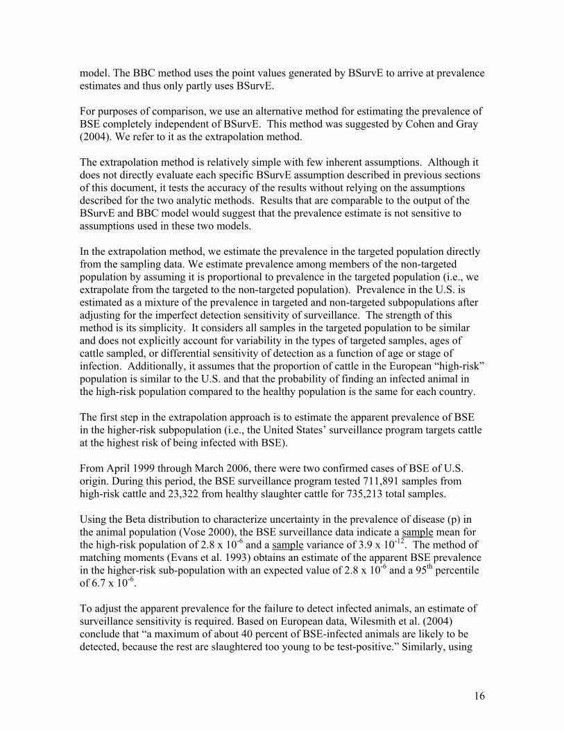
From April 1999 through March 2006, there were two confirmed cases of BSE of U.S. origin. During this period, the BSE surveillance program tested 711,891 samples from high-risk cattle and 23,322 from healthy slaughter cattle for 735,213 total samples. Using the Beta distribution to characterize uncertainty in the prevalence of disease (p) in the animal population (Vose 2000), the BSE surveillance data indicate a sample mean for the high-risk population of 2.8 x 10-6 and a sample variance of 3.9 x 10-12. The method of matching moments (Evans et al. 1993) obtains an estimate of the apparent BSE prevalence in the higher-risk sub-population with an expected value of 2.8 x 10-6 and a 95th percentile of 6.7 x 10-6. To adjust the apparent prevalence for the failure to detect infected animals, an estimate of surveillance sensitivity is required. Based on European data, Wilesmith et al. (2004) conclude that “a maximum of about 40 percent of BSE-infected animals are likely to be detected, because the rest are slaughtered too young to be test-positive.” Similarly, using

17

input data, age and production specific probability of exit, and incubation distribution from the Harvard-Tuskegee BSE risk model (Cohen et al., 2003) and assuming that animals become infected at 6 months, we calculate that 39.97 percent of BSE infected animals in the United States are expected to become clinical. Therefore, we assume that the sensitivity of the BSE surveillance is approximately 40 percent with respect to the higher-risk sub-population. Extrapolation from the high-risk sub-population to the normal sub-population requires an estimate of the relative likelihood of disease in the two sub-populations. Considering the BSE testing conducted in the EU-15 during 2001-2004 (available at: http://europa.eu.int/comm/food/food/biosafety/bse/annual_reps_en.htm), cattle in the European higher-risk population (emergency slaughter, clinical suspects, and fallen stock) are 28 times more likely to test BSE positive than cattle in the healthy slaughter category. To estimate prevalence in the total adult cattle population, a weighted average of the subpopulation estimates is calculated, where the weights assigned to the subpopulation values are their respective proportion of the total adult cattle population. Surveillance data are unavailable for a direct estimate of the proportion of the U.S. adult cattle population that satisfies the definition of animals at higher-risk of BSE. Nevertheless, APHIS (2004) estimated the cattle population targeted for BSE surveillance to be about 1 percent of the total U.S. adult cattle population. Although the structure of the cattle population and practices differ, the European Commission (EC) classified 3.26 percent and 3.42 percent of the European Union (EU) adult cattle population (≥ 2 years of age) as high risk (fallen stock, animals with clinical signs at ante mortem inspection, and emergency slaughter) in 2003 and 2004, respectively (EC 2004, 2005). Therefore, to maintain a conservative estimate (i.e., err on the side of higher prevalence), the higher-risk sub-population is assumed to represent 3 percent of the total adult cattle population. Accordingly, the normal sub-population is assumed to represent 97 percent of the total population4. Dividing the apparent prevalence distribution by the 40 percent sensitivity, then solving for the resultant beta distribution, gives an estimated prevalence distribution in the higher-risk sub-population. Applying the 1:28 ratio to the estimated BSE prevalence distribution in the higher-risk sub-population, then solving for the resultant beta distribution, estimates a prevalence in the normal sub-population. Simulating the weighted average of the higher-risk and normal subpopulations’ beta distributions estimates the mean, 5th, and 95th percentiles of the prevalence distribution. Sensitivity of prevalence estimate to additional cases The prevalence estimate in this analysis is based on two positive animals out of 735,213 samples. We add additional cases into the prevalence model input data without including any additional negative surveillance to provide perspective for the sensitivity of the prevalence estimate to additional BSE cases.

4 Note that if we assume that the higher-risk sub-population represents less than 3% of the total adult population, then the estimated prevalence in the total population will decrease. Therefore, our assumption of 3 percent will necessarily yield a higher estimate of BSE prevalence (i.e., this is a conservative assumption).

18

For example, the decision to exclude (or include) the positive Canadian-origin cow is problematic. Excluding this animal from the analysis is seemingly justified given that it was infected in Canada and its infection never threatened the U.S. cattle industry because it was destroyed when detected. Furthermore, the OIE recognizes this case as having been imported from Canada and assigns it to Canada (http://www.oie.int/eng/info/en_esbmonde.htm). Likewise, the detection of one or more additional cases is possible. Given the uncertainty inherent in the decision to exclude or include the Canadian-origin case and the possibility for detection of further cases, it is appropriate to assess the sensitivity of the estimated prevalence to the inclusion of additional positives. To examine this sensitivity, data reflecting one, two, or three new cases were added to the 1997 birth cohort test data (i.e., totals of three, four, or five cases), and alternative estimates of prevalence were generated by the BSurvE and Bayesian Birth Cohort methods. Sensitivity of prevalence estimate to alternatives for assumptions and input parameters to the BSurvE model. Sensitivity of prevalence estimate to changes in the likelihood ratio estimator for determining clinical suspects Two assumptions were made about the likelihood estimator used to assign samples from the enhanced surveillance to the clinical suspect surveillance stream. The first is the threshold value to assign the sample to the clinical suspect stream and the second relates to the inclusion of all surveillance data in the denominator of the likelihood ratio. Samples from the enhanced surveillance were initially defined as clinical suspects if they were submitted as being “highly suspicious” for BSE, rabies suspects, or animals that had CNS signs or were FSIS antemortem condemned for CNS signs. Many samples were submitted in other categories that also had a clinical history of signs likely to be associated with BSE but were not recorded as such in the “submission reason” section of the sample test form. Analysis of the enhanced BSE surveillance data identified these animals to be clinical suspects by comparing the likelihood of finding the signs in histopathologically confirmed cases reported in the U.K. (Wilesmith et al. 1992) with the likelihood of finding the signs in un-infected animals from the enhanced surveillance targeted population (APHIS 2006). For example, if a sign or combination of signs were found 30 percent of the time in BSE cases but only once in every 1,000 BSE negative animals (0.1 percent), then it would be 300 times (0.30/0.001) more likely to occur in the BSE cases. The threshold for assignment to the clinical suspect category was determined as samples from animals with signs that were at least 807 times more likely to be found in BSE cases than in the enhanced surveillance targeted population. For detailed description of the procedures used to allocate samples, see Summary of Enhanced BSE Surveillance in the United States (APHIS 2006).

19

To test the sensitivity of the prevalence estimate to the 807 threshold, we selected likelihood ratio cutoff values of 250 and 2000; 250 was the approximate 25th percentile of the points-by-age distribution (weighted by the frequency of various ages in the adult cattle population) and 2000 was approximately the largest point value assigned to a clinical suspect by the BSurvE model, respectively (APHIS 2006). Estimates from BSurvE and the Bayesian birth cohort methods were re-calculated using the revised number of clinical suspect samples resulting from the changes in likelihood ratio cutoffs. The second assumption about the likelihood ratio was that the denominator of the ratio correctly includes all negative surveillance data collected for enhanced surveillance although 84 percent had no observable clinical signs other than “dead-unknown cause” documented prior to death. The approach used in our baseline analysis assumes that all cattle reported “dead – unknown cause” had none of the clinical signs reported for submissions with more complete clinical histories. The approach in this sensitivity analysis is to assume that all cattle reported “dead – unknown cause” have clinical signs consistent with the frequency of clinical signs observed among those submissions with more complete clinical histories. This is equivalent to removing the “dead – unknown cause” submissions from the estimation of specificity (denominator of the likelihood ratio). Recalculation of the likelihood ratios for all cattle in the enhanced surveillance dataset was conducted for submissions that did not include “dead – unknown cause” as their sole clinical sign. Age determination At the time of sample collection, documentation of exact cattle ages was often not available, so cattle were primarily aged via dentition. With the exception of a five-month period in 2004, ages were recorded in a continuous fashion in years or months. The BSurvE model uses 17 different ages ranging from 1 to 17 in one-year increments (with age “1” representing cattle less than 2 years old, and “17” representing cattle aged 17 or older). Thus, our data were placed into one of these 17 age categories for use in the BSurvE model, as shown in Table 1. Ages were imputed as described in the document, Summary of Enhanced BSE Surveillance in the United States (APHIS 2006) for cattle of unknown age and for those collected during the 5-month period in which ages were recorded categorically Dentition is a relatively reliable indicator of age up to age 5, but it is difficult to accurately age cattle within one year of its true age for cattle aged 5 or older. Thus, it is likely that some ages were misclassified for cattle 5 or older. Because points in the BSurvE model are affected by cattle age, the sensitivity of the prevalence estimate to age is assessed in the sensitivity analysis. Additionally, ages for cattle 5 years or older were adjusted based on the probability of cattle of each age existing in the U.S. population (i.e., using data for cattle 5 and above in Table A2). This adjustment was performed prior to imputation of unknown cattle ages so the imputation could be based on the new age distribution.

20

Sensitivity of prevalence estimate to exit parameters affected by population age distribution, pre-clinical detection, and probabilities that uninfected and infected cattle will exit via each surveillance stream The BSurvE model depends on several inputs that are difficult to estimate. For example, the proportion of infected cattle that exit via each of the four surveillance streams is impossible to determine in the United States because of the small number of infected cattle. The BSurvE model provides values for such inputs based on scientific literature and data from the U.K. and European outbreaks. Additionally, the BSurvE developers have designed a tool to assess the sensitivity of prevalence estimates to changes in input settings and model parameters. The tool, BSens, is an Excel® (Microsoft Corporation, Redmond, WA) spreadsheet application. (BSens was provided by the BSurvE authors August 2005: available by request at http://www.BSurvE.com) BSens allows sensitivity analysis on:

a) Exit probability parameters affected by population age distribution (e.g., exit probabilities for uninfected (BSurvE variable Dt) and infected (BSurvE variable Ct) cattle at age t.

b) The proportion of preclinical cattle that exit and are detectable. c) Probabilities that uninfected (BSurvE variable tjd , ) and infected (BSurvE

variable tjc , ) cattle will exit via surveillance stream j given that they exit at time t.

The U.S. testing data used for the BSurvE analysis were summarized and entered into BSens including the age distribution of cattle used for the U.S. analysis (as outlined in Appendix A). BSens analyzes sensitivity using the Prevalence B algorithm. As BSurvE inputs are changed in BSens, the percentage change in prevalence is measured relative to the baseline result. Using regression analysis, BSens estimates sensitivity coefficients, which equal the percentage change in prevalence for a 1 percent change in the value of the input. A large coefficient suggests that estimated prevalence is relatively sensitive to the input while smaller coefficients suggest less influential inputs.

a) Exit probability parameters influenced by population age distribution; Exit probabilities for uninfected (Dt) and infected (Ct) cattle at age t.

The cattle age distribution used in BSurvE is an input provided by the user that describes the number of cattle by age in the United States cattle population and determines the annual culling fraction for all integer ages of cattle (Dt). The age-related culling fraction is a crucial input to calculating the point values of samples in BSurvE. To assess the sensitivity of estimated prevalence to changes in the exit parameter Dt (directly calculated from cattle age distribution), a gamma distribution is fit to the cattle age distribution . Although the actual U.S. distribution is not best described by a gamma distribution, Bsens only requires an approximate fit to calculate the relative differences reported by sensitivity analysis. The mean,

21

standard deviation, and mode of the fitted gamma distribution are systematically altered and the change in estimated prevalence is recorded by BSens. In similar manner, to assess the sensitivity of estimated prevalence to changes in the latent period for infected cattle (Ct), BSens fits a gamma distribution to the age distribution used in BSurvE. The mean, standard deviation and mode of this gamma distribution are systematically altered to assess the sensitivity of prevalence to this input.

b) Proportion of exiting preclinical cattle that are detectable.

The value used in BSurvE for the proportion of preclinical cattle that are detectable within 1 year of developing clinical disease is 40 percent. BSens evaluates the sensitivity of prevalence by changing this value and calculating a coefficient of sensitivity.

c) Probabilities (proportions) that uninfected (dj,t) and infected (cj,t) cattle will exit via

each surveillance stream (j) given that they exit at time t (from BSurvE table 4 and 5).

By altering the probabilities that infected animals exit via one of the surveillance streams given that it leaves at age t (cj,t) for the healthy slaughter, fallen stock and casualty slaughter streams, BSens determines the sensitivity of prevalence estimates to all of these inputs. The clinical suspect probabilities are adjusted on each iteration of BSens so that the total exit probability for each age category sums to one. By altering the probabilities that uninfected animals exit via one of the surveillance streams given that it leaves at age category t (dj,t) for the healthy slaughter, fallen stock and casualty slaughter streams, BSens determines the sensitivity of prevalence estimates to all of these inputs. The clinical suspect values are adjusted on each iteration of BSens so that the total probability for each age sums to one.

Results of Prevalence Analysis

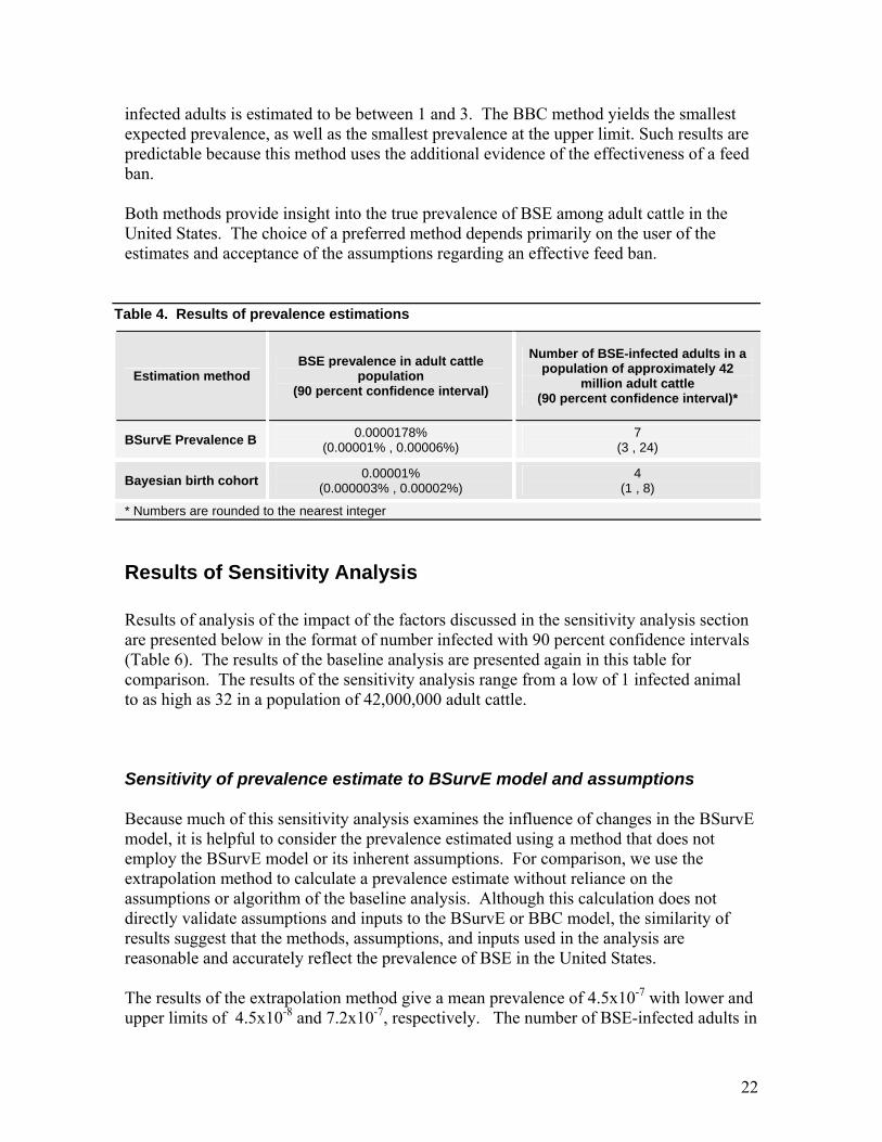
Results of prevalence analysis For each of the two methods used in the analysis, the expected prevalence and the 90 percent confidence limits are shown in Table 4. The corresponding number of infected animals among the approximately 42 million adult cattle in the United States is also estimated for the expected prevalence as well as the 90 percent confidence interval. The results of the two methods are similar, with the expected number of infected adults at 4 and 7 respectively for BBC and BSurvE Prevalence B. At the upper limit, the number of infected adults is estimated to be between 8 and 24; while at the lower limit, the number of

22

infected adults is estimated to be between 1 and 3. The BBC method yields the smallest expected prevalence, as well as the smallest prevalence at the upper limit. Such results are predictable because this method uses the additional evidence of the effectiveness of a feed ban. Both methods provide insight into the true prevalence of BSE among adult cattle in the United States. The choice of a preferred method depends primarily on the user of the estimates and acceptance of the assumptions regarding an effective feed ban.

Table 4. Results of prevalence estimations

Estimation method BSE prevalence in adult cattle

population (90 percent confidence interval)

Number of BSE-infected adults in a population of approximately 42

million adult cattle (90 percent confidence interval)*

BSurvE Prevalence B 0.0000178% (0.00001% , 0.00006%)

7 (3 , 24)

Bayesian birth cohort 0.00001% (0.000003% , 0.00002%)

4 (1 , 8)

* Numbers are rounded to the nearest integer Results of Sensitivity Analysis

Results of analysis of the impact of the factors discussed in the sensitivity analysis section are presented below in the format of number infected with 90 percent confidence intervals (Table 6). The results of the baseline analysis are presented again in this table for comparison. The results of the sensitivity analysis range from a low of 1 infected animal to as high as 32 in a population of 42,000,000 adult cattle. Sensitivity of prevalence estimate to BSurvE model and assumptions Because much of this sensitivity analysis examines the influence of changes in the BSurvE model, it is helpful to consider the prevalence estimated using a method that does not employ the BSurvE model or its inherent assumptions. For comparison, we use the extrapolation method to calculate a prevalence estimate without reliance on the assumptions or algorithm of the baseline analysis. Although this calculation does not directly validate assumptions and inputs to the BSurvE or BBC model, the similarity of results suggest that the methods, assumptions, and inputs used in the analysis are reasonable and accurately reflect the prevalence of BSE in the United States. The results of the extrapolation method give a mean prevalence of 4.5x10-7 with lower and upper limits of 4.5x10-8 and 7.2x10-7, respectively. The number of BSE-infected adults in

23

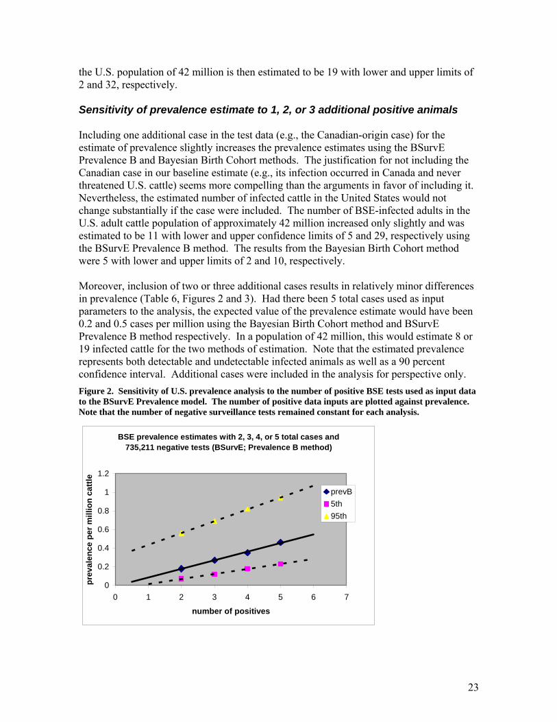
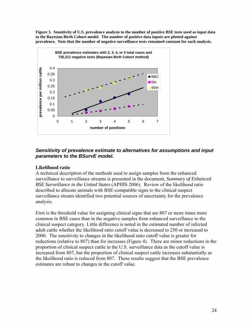
the U.S. population of 42 million is then estimated to be 19 with lower and upper limits of 2 and 32, respectively. Sensitivity of prevalence estimate to 1, 2, or 3 additional positive animals Including one additional case in the test data (e.g., the Canadian-origin case) for the estimate of prevalence slightly increases the prevalence estimates using the BSurvE Prevalence B and Bayesian Birth Cohort methods. The justification for not including the Canadian case in our baseline estimate (e.g., its infection occurred in Canada and never threatened U.S. cattle) seems more compelling than the arguments in favor of including it. Nevertheless, the estimated number of infected cattle in the United States would not change substantially if the case were included. The number of BSE-infected adults in the U.S. adult cattle population of approximately 42 million increased only slightly and was estimated to be 11 with lower and upper confidence limits of 5 and 29, respectively using the BSurvE Prevalence B method. The results from the Bayesian Birth Cohort method were 5 with lower and upper limits of 2 and 10, respectively. Moreover, inclusion of two or three additional cases results in relatively minor differences in prevalence (Table 6, Figures 2 and 3). Had there been 5 total cases used as input parameters to the analysis, the expected value of the prevalence estimate would have been 0.2 and 0.5 cases per million using the Bayesian Birth Cohort method and BSurvE Prevalence B method respectively. In a population of 42 million, this would estimate 8 or 19 infected cattle for the two methods of estimation. Note that the estimated prevalence represents both detectable and undetectable infected animals as well as a 90 percent confidence interval. Additional cases were included in the analysis for perspective only. Figure 2. Sensitivity of U.S. prevalence analysis to the number of positive BSE tests used as input data to the BSurvE Prevalence model. The number of positive data inputs are plotted against prevalence. Note that the number of negative surveillance tests remained constant for each analysis.

BSE prevalence estimates with 2, 3, 4, or 5 total cases and 735,211 negative tests (BSurvE; Prevalence B method)

0

0.2

0.4

0.6

0.8

1

1.2

0 1 2 3 4 5 6 7

number of positives

prev

alen

ce p

er m

illio

n ca

ttle

prevB5th95th

24

Figure 3. Sensitivity of U.S. prevalence analysis to the number of positive BSE tests used as input data to the Bayesian Birth Cohort model. The number of positive data inputs are plotted against prevalence. Note that the number of negative surveillance tests remained constant for each analysis.

BSE prevalence estimates with 2, 3, 4, or 5 total cases and 735,211 negative tests (Bayesian Birth Cohort method)

00.050.1

0.150.2

0.250.3

0.350.4

0 1 2 3 4 5 6 7

number of positives

prev

alen

ce p

er m

illio

n ca

ttle

BBC5th95th

Sensitivity of prevalence estimate to alternatives for assumptions and input parameters to the BSurvE model. Likelihood ratio A technical description of the methods used to assign samples from the enhanced surveillance to surveillance streams is presented in the document, Summary of Enhanced BSE Surveillance in the United States (APHIS 2006). Review of the likelihood ratio described to allocate animals with BSE-compatible signs to the clinical suspect surveillance stream identified two potential sources of uncertainty for the prevalence analysis. First is the threshold value for assigning clinical signs that are 807 or more times more common in BSE cases than in the negative samples from enhanced surveillance to the clinical suspect category. Little difference is noted in the estimated number of infected adult cattle whether the likelihood ratio cutoff value is decreased to 250 or increased to 2000. The sensitivity to changes in the likelihood ratio cutoff value is greater for reductions (relative to 807) than for increases (Figure 4). There are minor reductions in the proportion of clinical suspect cattle in the U.S. surveillance data as the cutoff value is increased from 807, but the proportion of clinical suspect cattle increases substantially as the likelihood ratio is reduced from 807. These results suggest that the BSE prevalence estimates are robust to changes in the cutoff value.

25

0

0.01

0.02

0.03

0.04

0.05

0.06

0.07

0.08

0.09

0.1

1 10 100 1,000 10,000 100,000 1,000,000 10,000,000

Likelihood value (log scale)

Prop

ortio

n of

cat

tle w

ith li

kelih

ood

>1

Figure 4. Plot of likelihood ratio values for cattle in the U.S. enhanced BSE surveillance database with estimated likelihood ratios greater than one.

The second source of uncertainty in the likelihood ratio was the inclusion of all negative surveillance data in the ratio’s denominator. The number of clinical suspects was recalculated after animals with the single presenting sign of “dead-unknown cause” were excluded from the denominator. The recalculated likelihood ratios were uniformly smaller than those calculated in the baseline analysis resulting in fewer samples with values that exceed the threshold of 807 necessary to qualify as clinical suspects. In the baseline analysis, there were 5,771 samples classified as clinical suspects. In this sensitivity analysis, this count was revised to 5,013. The sensitivity of prevalence to the recalculated values was low. Age determination Because age determination of cattle by changes in dentition becomes increasingly less precise after age 5 years, the possibility exists that the reported ages of cattle in the surveillance data were incorrectly recorded. Redistributing the reported ages for cattle 5 and above to parallel the distribution of cattle aged 5 and above in the standing population resulted in a more even distribution of samples across the ages 5-17. However, this had little effect on prevalence estimates, raising it only slightly. Sensitivity of prevalence estimate to exit parameters dependent on age distribution (BSurvE variables Dj,t and Cj,t), pre-clinical detection, and probabilities (proportions) that uninfected and infected cattle will exit via each surveillance stream

26

Exit constants for uninfected and infected cattle (Dj,t and Cj,t) The age distribution input to BSurvE for the United States is described in detail in Appendix A. This input is used by BSurvE to calculate exit constants of uninfected animals (Dt). The Bsens sensitivity coefficient suggests that small changes will result in small changes in prevalence. We have a high degree of certainty that this input is correct for the United States’ cattle population and consider this potential source of uncertainty unlikely to have substantial impact on the results of the analysis. The Bsens coefficients for Dt suggest that BSE prevalence estimated by BSurvE changes approximately proportional to changes in the mean and standard deviation of the gamma distribution describing Dt. For example, a 1 percent increase in the mean of the gamma distribution for Dt results in a 1.5 percent increase in prevalence. If the average age of uninfected cattle increases, then the points per sample is generally reduced; this change will render U.S. surveillance evidence slightly less valuable and imply a slightly larger prevalence. In contrast, a 1 percent increase in the standard deviation of the gamma distribution for Dt results in a 1.9 percent decrease in prevalence. Therefore, if the spread of the culling distribution is increased, then the culling fraction for the middle ages of cattle tends to be reduced; this change will increase likelihood ratios for middle-aged cattle (e.g., 4- to 6-year-olds) thereby increasing the point values for such samples and implying a slightly smaller prevalence. The exit probabilities for infected animals (Ct inputs) are also influenced by age distribution but cannot be estimated from U.S. data because of the lack of positive animals. Because disease specific parameters such as latency period are unlikely to vary between countries, the values used in BSurvE are assumed the most appropriate exit constants. The sensitivity coefficient for Ct suggests that BSE prevalence estimated by BSurvE will increase by approximately 3.3 percent for a 1 percent increase in the mean of the latency period. Increasing the average age that infected cattle exit the population (latency period) will generally reduce the point values of samples and, correspondingly, cause the surveillance information to support a somewhat larger prevalence. On the other hand, increasing the standard deviation by 1 percent increases the spread of the distribution and results in almost a 1 percent decrease in prevalence. The sensitivity coefficients for these inputs were low, so changing these inputs would not result in disproportionately large changes in prevalence. Proportion of exiting preclinical cattle that are detectable The probability that pre-clinical cattle are detectable within 1 year of developing clinical signs had a very small sensitivity coefficient and negligible effect on the prevalence estimate. The sensitivity coefficient estimated by BSens for this parameter is -2.3x10-11.

27

Probabilities (proportions) that uninfected (BSurvE variable dj,t) and infected (BSurvE variable cj,t) cattle will exit via each surveillance stream (j) given that they exit at time t (from BSurvE table 4 and 5). The sensitivity coefficients estimated by BSens describe the percentage change in prevalence for a 1 percent change in the surveillance stream exit probabilities for infected cattle (cj,t) and uninfected cattle (dj,t). The coefficients for the cj,t parameters suggest that BSE prevalence has low sensitivity to these parameters. For example, a 10 percent increase in the proportion of infected cattle that exit via the healthy slaughter stream (e.g., from 5 percent to 5.5 percent) will increase prevalence by approximately 0.5 percent (~10 x 0.05 percent). Nevertheless, the BSurvE values for cj,t (generally 5 percent, 10 percent, 10 percent, and 75 percent for healthy, fallen stock, casualty slaughter and clinical suspect surveillance streams, respectively), were derived from a combination of U.K. and E.U. data, as well as expert opinion (D. Prattley, personal communication, 2006). For the U.S. prevalence analysis, these values were deemed a reasonable approximation of the streams in which BSE-infected cattle showing signs would exit. A review of recent E.U. BSE surveillance data (excluding the U.K.) suggests that the proportion of infected cattle exiting the population as clinical suspects may be smaller than the BSurvE values. The U.K. was excluded from the aforementioned review of E.U. surveillance data because of differences from other E.U. countries, including more infected clinical suspect cases because of that country’s past reliance on passive reporting of suspicious BSE cases. The stream in which infected animals, if present in the U.S., would likely exit the U.S. herd is debatable and based on epidemiology, management, and culling practices. However, using the E.U. proportions for infected cattle exiting via each surveillance stream appears to be one reasonable alternative for the BSurvE values of cj,t, so this was included in the sensitivity analysis. Based on 2004 E.U. data (after subtraction of U.K. results) exit fractions for the healthy slaughter, fallen stock, casualty slaughter and clinical suspect streams were 29 percent, 49 percent, 2 percent, and 20 percent, respectively.. These values were used for cj,t, in place of the aforementioned 5 percent, 10 percent, 10 percent, and 75 percent for healthy, fallen stock, casualty slaughter and clinical suspect surveillance streams, respectively. The cj,t values are intended to be estimates of how animals would leave the standing population if they were infected and showing clinical signs. Looking at the animals testing positive in each surveillance stream includes those that are clinically as well as preclinically infected (except for those in the clinical suspect stream). Thus the percentages of animals testing positive in each stream cannot be directly used for cj,t. Nevertheless, using the E.U. data provides a quantified scenario for further testing the sensitivity of prevalence to this input. Despite the reduction in fraction of infected cattle exiting via the clinical suspect stream in this alternative scenario, the resulting estimated prevalence is only moderately increased. The coefficients for the dj,t parameters demonstrate that BSE prevalence estimated by BSurvE is more sensitive to these parameters than others assessed in this section. For

28

example, a 1 percent increase in the proportion of uninfected cattle that exit via the healthy slaughter stream (e.g., from 87.8 percent to 88.7 percent) will decrease prevalence by approximately 3 ½ fold. But, an increase of this magnitude for the healthy slaughter stream also changes the other exit probabilities by approximately -7 percent, which has the overall effect of increasing prevalence by approximately 2 ¼ fold (e.g., 0.2 per million to 0.5 per million) because of the much larger reduction in exit constants for fallen stock, casualty slaughter and clinical suspects. Nevertheless, such results are not intuitively appealing because we expect a reduction in the exit constant for, particularly, clinical suspects to result in a reduction in prevalence5. One problem with the BSens approach for dj,t is that the exit constant for the healthy slaughter stream is close to one, so even small changes to this value require drastic changes in the other exit constant values. To clarify this sensitivity we can directly observe changes in prevalence by changing the BSurvE settings according to uncertainties that are specific to the U.S. situation (i.e., identify what values of dj,t are implied by the U.S. surveillance evidence). The values for dj,t vary according to cattle age. For example, the probability of uninfected cattle leaving via the healthy slaughter stream varies from 97 percent the first year of age to 87.8 percent for 16-year-old cattle. Similarly, the probability such cattle exit via the clinical suspect category increases from 0.01 percent during the first year to 0.1 percent at 16 years of age. Because the U.S. surveillance effort did not target healthy slaughter cattle, it is not possible to assess the probability of this path from our sample. Nevertheless, if we recalculate the dj,t probabilities conditioned on sampling strictly from the fallen stock, casualty slaughter and clinical suspect streams, we estimate the fraction of samples expected from each stream according to the BSurvE settings. Similarly, we can calculate the relative frequency of samples from the U.S. surveillance effort in each of these targeted streams. The results of this comparison do not exactly overlap, but the overall frequency of clinical suspects sampled is similar to what the BSurvE values for dj,t would predict (Table 5).

5 Points per sample collected from an animal in surveillance stream j of age t is calculated as

,,

,

j tj t

j t

gv

d= (see Appendices A and B). If the denominator of this expression for the clinical suspect stream

is reduced, then we expect the point value per sample to increase thereby reducing the estimated prevalence in the population because of a larger implied sample size.

29

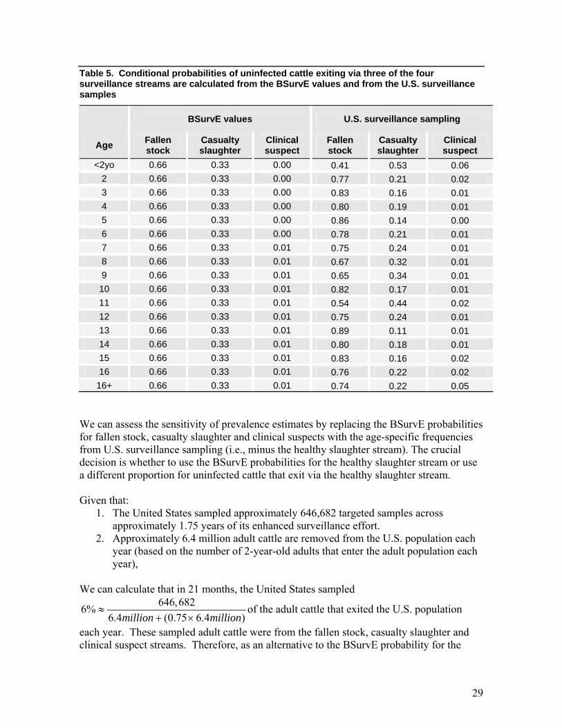
Table 5. Conditional probabilities of uninfected cattle exiting via three of the four surveillance streams are calculated from the BSurvE values and from the U.S. surveillance samples

BSurvE values U.S. surveillance sampling

Age Fallen stock

Casualty slaughter

Clinical suspect

Fallen stock

Casualty slaughter

Clinical suspect

<2yo 0.66 0.33 0.00 0.41 0.53 0.06 2 0.66 0.33 0.00 0.77 0.21 0.02 3 0.66 0.33 0.00 0.83 0.16 0.01 4 0.66 0.33 0.00 0.80 0.19 0.01 5 0.66 0.33 0.00 0.86 0.14 0.00 6 0.66 0.33 0.00 0.78 0.21 0.01 7 0.66 0.33 0.01 0.75 0.24 0.01 8 0.66 0.33 0.01 0.67 0.32 0.01 9 0.66 0.33 0.01 0.65 0.34 0.01 10 0.66 0.33 0.01 0.82 0.17 0.01 11 0.66 0.33 0.01 0.54 0.44 0.02 12 0.66 0.33 0.01 0.75 0.24 0.01 13 0.66 0.33 0.01 0.89 0.11 0.01 14 0.66 0.33 0.01 0.80 0.18 0.01 15 0.66 0.33 0.01 0.83 0.16 0.02 16 0.66 0.33 0.01 0.76 0.22 0.02

16+ 0.66 0.33 0.01 0.74 0.22 0.05 We can assess the sensitivity of prevalence estimates by replacing the BSurvE probabilities for fallen stock, casualty slaughter and clinical suspects with the age-specific frequencies from U.S. surveillance sampling (i.e., minus the healthy slaughter stream). The crucial decision is whether to use the BSurvE probabilities for the healthy slaughter stream or use a different proportion for uninfected cattle that exit via the healthy slaughter stream. Given that:

1. The United States sampled approximately 646,682 targeted samples across approximately 1.75 years of its enhanced surveillance effort.

2. Approximately 6.4 million adult cattle are removed from the U.S. population each year (based on the number of 2-year-old adults that enter the adult population each year),

We can calculate that in 21 months, the United States sampled

646,6826%6.4 (0.75 6.4 )million million

≈+ ×

of the adult cattle that exited the U.S. population

each year. These sampled adult cattle were from the fallen stock, casualty slaughter and clinical suspect streams. Therefore, as an alternative to the BSurvE probability for the

30

healthy slaughter streams, we might estimate that the average probability for the healthy slaughter stream among U.S. cattle was approximately 94 percent. If the BSurvE probabilities for the healthy slaughter stream are used with the U.S. surveillance test results, then the age-specific unconditional probabilities for fallen stock, casualty slaughter and clinical suspects must be calculated. In this case, the resulting prevalence estimates are slightly larger than our baseline estimates. If we use a probability of 94 percent for the healthy slaughter stream and the U.S. surveillance sampling results, then the BSurvE Prevalence B and Bayesian birth cohort methods predict prevalence levels that are less than our baseline estimates.

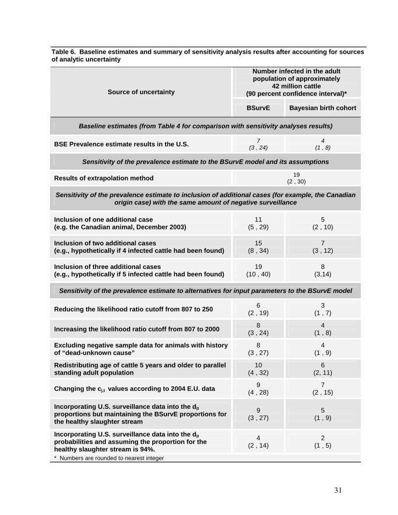
31

Table 6. Baseline estimates and summary of sensitivity analysis results after accounting for sources of analytic uncertainty

Number infected in the adult population of approximately

42 million cattle (90 percent confidence interval)* Source of uncertainty

BSurvE Bayesian birth cohort

Baseline estimates (from Table 4 for comparison with sensitivity analyses results)

BSE Prevalence estimate results in the U.S. 7 (3 , 24)

4 (1 , 8)

Sensitivity of the prevalence estimate to the BSurvE model and its assumptions

Results of extrapolation method 19 (2 , 30)

Sensitivity of the prevalence estimate to inclusion of additional cases (for example, the Canadian origin case) with the same amount of negative surveillance

Inclusion of one additional case (e.g. the Canadian animal, December 2003)

11 (5 , 29)

5 (2 , 10)

Inclusion of two additional cases (e.g., hypothetically if 4 infected cattle had been found)

15 (8 , 34)

7 (3 , 12)

Inclusion of three additional cases (e.g., hypothetically if 5 infected cattle had been found)

19 (10 , 40)

8 (3,14)

Sensitivity of the prevalence estimate to alternatives for input parameters to the BSurvE model

Reducing the likelihood ratio cutoff from 807 to 250 6 (2 , 19)

3 (1 , 7)

Increasing the likelihood ratio cutoff from 807 to 2000 8 (3 , 24)

4 (1 , 8)

Excluding negative sample data for animals with history of “dead-unknown cause”

8 (3 , 27)

4 (1 , 9)

Redistributing age of cattle 5 years and older to parallel standing adult population

10 (4 , 32)

6 (2, 11)

Changing the cj,t values according to 2004 E.U. data 9 (4 , 28)

7 (2 , 15)

Incorporating U.S. surveillance data into the djt proportions but maintaining the BSurvE proportions for the healthy slaughter stream

9 (3 , 27)

5 (1 , 9)

Incorporating U.S. surveillance data into the djt probabilities and assuming the proportion for the healthy slaughter stream is 94%.

4 (2 , 14)

2 (1 , 5)

* Numbers are rounded to nearest integer

32

Conclusion of Analysis

The United States has conducted BSE surveillance with increasing intensity since 1990, including an enhanced effort following the identification of a Canadian cow that tested positive in 2003 (APHIS 2006). This analysis uses surveillance data that have been collected over the 7-year period prior to March 17, 2006, to estimate the prevalence of BSE in the United States. The first part of the prevalence analysis required test samples allocated into surveillance streams compatible with the BSurvE model (Wilesmith et al. 2004, Wilesmith et al 2006). The procedures and limitations of sample collection and allocation have been previously described in detail in the document, Summary of Enhanced BSE Surveillance in the United States (APHIS 2006). We use as a basis for our prevalence estimates the BSurvE model (Wilesmith et al. 2004). The BSurvE model is noteworthy for its sound epidemiologic structure, including stratifying cattle by age and cause of death and accounting for the relative likelihood of detecting BSE in various strata (EFSA 2004). It combines surveillance data, population demographics, and knowledge of the disease pathogenesis with evidence of the relative likelihoods of infectivity in various sub-populations, to estimate BSE prevalence in the entire cattle population. Moreover, the prevalence estimate includes all infected cattle regardless of whether they demonstrated clinical signs, or had been tested for BSE. Prevalence was estimated using two methods. The first estimate from the BSurvE model Prevalence B worksheet is based only on surveillance testing data with no additional information about an effective feed ban. The second method (Bayesian Birth Cohort model) uses the point assignments from the BSurvE model and assumes that the U.S. feed ban was at least as effective as the initial (1988) U.K. ban; i.e., that prevalence would decline proportionately. The mathematical techniques used in this method combine the surrogate U.K. information with surveillance data to provide a more precise estimation of the expected prevalence in the United States. Many inputs for these analyses required assumptions, estimates, or the use of uncertainty distributions. The implications of these uncertain values are discussed in detail in the text. The determination of uncertain parameters was based on justifiable “most likely values” where possible and plausible but conservative estimates otherwise. Additionally, a sensitivity analysis was conducted on several parameters with potential to have significant effect on the models. In each case, the magnitude of change due to the uncertain parameters was not substantial and did not change the conclusion that the prevalence of BSE is less than 1 case per million adult cattle. The results presented are intended to provide an estimate of prevalence based on the best available data and most likely assumptions for unknown parameters. Among the 735,213 cattle sampled in the 7 years prior to March 17, 2006, two infected indigenous animals were identified by the surveillance in addition to the 2003 imported cow from Canada. The results of the two methods of analysis suggest that the number of

33

infected cattle in the United States is extremely low. The 90 percent confidence interval of BSE infected cattle for the two models was between 1 and 8 and between 3 and 24 in a population of approximately 42,000,000 adult cattle. The data were re-analyzed to determine the sensitivity of the prevalence estimate to:

1. The BSurvE model and its assumptions 2. Inclusion of additional cases (e.g., the Canadian origin case) with the same amount

of negative surveillance, 3. Alternatives for assumptions and input parameters to the BSurvE model.

The range of outcomes from these analyses was 1 to 32 infected animals.6 The upper and lower bound of the estimates (range 1 to 32) are a very small fraction of the total population, and strongly support a conclusion that the prevalence of BSE in the United States is below 1 case per million adult cattle. Furthermore, this conclusion remains robust even if as many as five infected cattle had been included in the analysis with no additional negative surveillance data.

6 Table 6 presents two analyses in which the upper bound is greater than 32 infected cattle. However, these are hypothetical situations in which more than 3 cases of BSE are identified in the U.S. These analyses were conducted to show the robustness of the prevalence estimate given the amount of surveillance data that has been collected.

34

Appendix A: Age Distribution of U.S. Cattle

Age distribution of the U.S. national herd The age distribution of cattle is an input parameter to the BSurvE model used to estimate the rate that normal cattle leave the population, and thereby has considerable influence on its estimation of prevalence. Although the United States has begun implementation of a National Animal Identification System (NAIS), the age distribution of cattle has not been fully documented. The following paragraphs describe the derivation of the age distribution used for the BSE analysis. Beef cattle age distribution Rohrer et al. (1988) followed a herd composed of both purebred and mixed-breed cattle throughout their lifetimes and documented the ages that the animals were removed for reproductive failure, death, or disease. Unlike dairy animals, beef cattle are generally maintained in the breeding herd until they fail to produce a calf, which results in a considerably older population. In the Rohrer study, the average age of culling was 9.5 years. The survival analysis conducted on these animals determined that a Weibull distribution would best fit the data with the probability of survival until time “t” equal to the function:

p(t) = exp((-λ t)γ)

The average of the parameters for all cattle of the reported data were:

scale = λ = 0.086 and shape = γ = 2.69. The number of 1-year-olds in the U.S. population of breeding animals was estimated to be equal to the 5,746,000 replacement heifers reported in the NASS database (NASS 2005 ) for January 2005. The number of 2-year-old animals was estimated to be the number of 1-year-olds, minus the probability of culling for first-year heifers. This number is relatively high as maturing heifers are culled during breeding and gestation, but is not readily available in published literature. However, a reasonable estimate of the 2-year-old adult breeding population is reflected by the number of heifers expected to calve as reported by NASS (NASS 2005). For 2005, there were 3,568,000 expected to calve, which suggests that about 38 percent of calves set aside as replacement heifers never enter the adult herd. The number of calves that would eventually enter the replacement heifer cohort would reflect the number of replacement heifers plus the death loss in the first year. Beef calf death loss prior to weaning was estimated by USDA/NAHMS to be 5.5 percent (NAHMS 1998). A small number of calves would be expected to die between weaning and the time they would be chosen as replacements. The Harvard-Tuskegee Study used an annual death rate of 1.2 percent throughout a beef animal’s life (Cohen et al. 2001, 2003). The NAHMS study reported an annual mortality rate of 1.5 percent. Since there is no specific time that replacement heifers are chosen for culling, it is estimated that the death rate between weaning and replacement culling would be 1 percent. Thus, the 0 to 1 age

35

cohort would be 5,746,000 + (0.065*5,746,000) = 6,119,490. The number of animals in the remaining age groups was estimated using the survival function shown above and the starting adult cohort size (2 years) of 3,568,000. The beef cow age distribution as described above resulted in the numbers shown in Table A2. Note that approximately two-thirds of the animals are predicted to be culled after age 8. This is compatible with the NAHMS reason for culling data (NAHMS 1997). The results of the survey indicate that 39 percent of beef cattle were culled because of age or bad teeth. Another 32.9 percent were culled for reproductive reasons or poor calves, reasons that in most cases correspond to older animals. Also, note that the total number predicted by this age distribution (33,038,725) is very similar to NASS data (i.e., 33,055,000 for January 2005). Dairy cattle age distribution The dairy population distribution was reconstructed using summary data provided by Dairy Herd Improvement Association (DHIA) lactation records from Raleigh, NC, and Provo, UT. Animals were assumed to enter first lactation at age 2 and to have one lactation per year afterward until culled. The two milk sheds were assumed to reasonably predict the dairy population in the rest of the United States, and the proportion of animals at each age was extrapolated to the total number of dairy cattle reported by NASS 2005 (9,005,000 milk cows). The number of replacement heifers was taken from NASS data and the assumption made that replacement heifers were 1 year old. The number of animals culled between age 1 and 2 was taken as the difference of the number of replacements (NASS 2005) and the proportion of 2-year-olds predicted by the DHIA records. Since the number of animals entering the population greatly influences the distribution, the ratio of replacements to the number of heifers expected to calve was cross-checked against NASS data (NASS 2005) and the number of first lactation heifers reported in the NASS/NAHMS non-ambulatory study. This ratio was 0.312 for the NAHMS non-ambulatory study (Table A1), 0.315 from NASS statistics, and 0.317 for the DHIA ratio used in the age distribution estimate. Additionally, the number of cattle culled in 1 year, plus the death loss, would be expected to approximate the number of 2-year-olds that enter the herd each year. The NAHMS Dairy Study of 2002 (NAHMS 2002) reports the percent of cows culled for the year was 25.5 percent and the death loss was 4.8 percent. The sum of these numbers is 30.3 percent, which further supports the estimated number of 2-year-olds in the dairy population to be about 30 percent of the adult population. Finally, although the non-ambulatory study did not detail animals by age, the proportions of second, third, and fourth lactations and five or greater lactations compared reasonably well to the proportions predicted by the DHIA distribution. However, the DHIA-based data describe a slightly younger population than the NAHMS cross sectional survey. The difference may be due to several factors. First, the numbers represent slightly different measures; the NAHMS study reports proportions of animals in herds from a cross sectional survey, which could bias the results toward smaller and less intensive

36

production herds. A second possibility could be recall bias for producers who participated in the survey without consulting records for the actual proportions of their herd in each lactation. Alternatively, the DHIA distribution may be biased toward larger high production herds, which might describe a younger population. The DHIA-based distribution was chosen without modification for the following reasons. First, it is derived from actual recorded data rather than survey responses. Secondly, the difference is relatively small. And finally, the younger distribution will err conservatively in the BSurvE point value calculations. Table A1. Comparison of lactation data from NAHMS study to estimate of distribution used for BSE analysis. Note that approximately 80% of the herds reported in the NAHMS study are represented in the first column.

Lactation Percent of non-ambulatory herd

Percent of control herd

Distribution used in BSE analysis

1st 31.2% 25.8% 31.7% 2nd , 3rd , and 4th 48.8% 48% 56.0%

5th or greater 20% 26.2% 12.3% Comparison of number entering population to culling and death losses The estimated age distribution shown in Table A2 reasonably models the number of animals expected to enter the national herd based on the number of cull cattle and the death losses. For example, the number of federally inspected slaughter cattle reported in 2004 was 5,069,000. The beef death loss described above at 1.5 percent would be approximately 0.015*33,038,725 =495,580. Dairy death loss as described above would be approximately 0.048*9,004,976 = 432,239. The total would then be approximately 6 million. The difference from the 6,439,494 2-year-olds reported in Table A2 is likely due to other NASS slaughter reporting categories such as “farm slaughter” (154,000) and “other (commercial)” slaughter (587,000) (NASS 2005).

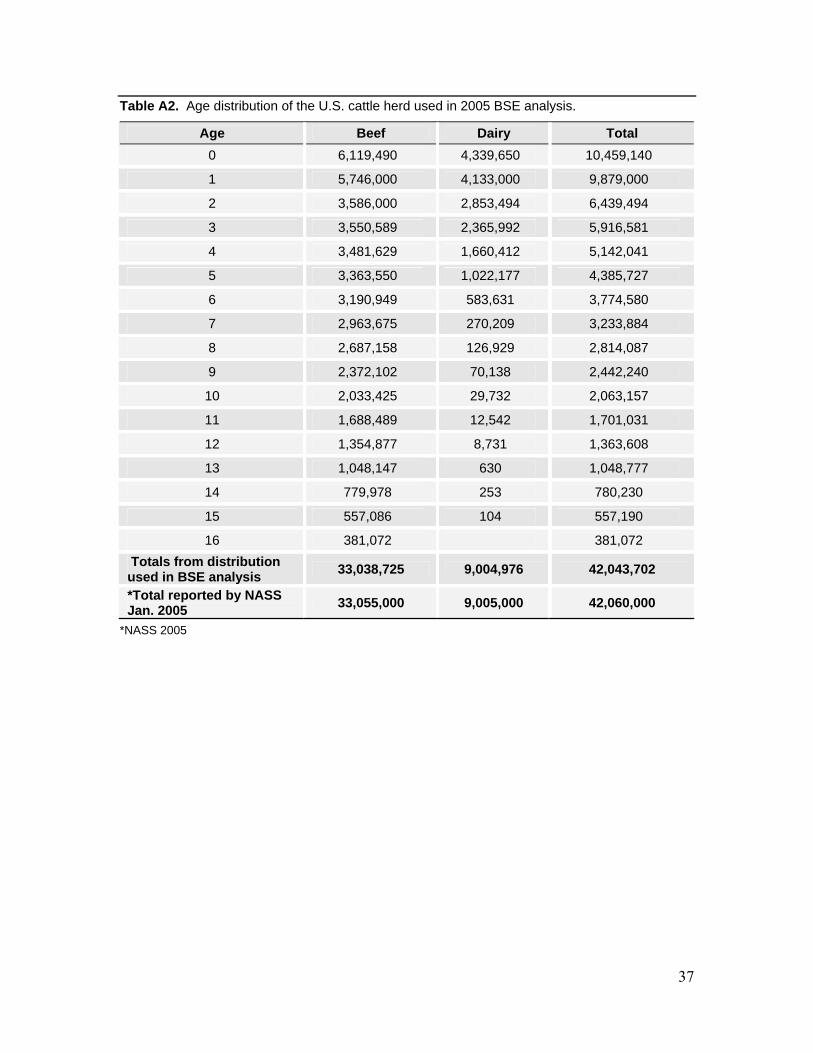
37

Table A2. Age distribution of the U.S. cattle herd used in 2005 BSE analysis.

Age Beef Dairy Total 0 6,119,490 4,339,650 10,459,140

1 5,746,000 4,133,000 9,879,000

2 3,586,000 2,853,494 6,439,494

3 3,550,589 2,365,992 5,916,581

4 3,481,629 1,660,412 5,142,041

5 3,363,550 1,022,177 4,385,727

6 3,190,949 583,631 3,774,580

7 2,963,675 270,209 3,233,884

8 2,687,158 126,929 2,814,087

9 2,372,102 70,138 2,442,240

10 2,033,425 29,732 2,063,157

11 1,688,489 12,542 1,701,031

12 1,354,877 8,731 1,363,608

13 1,048,147 630 1,048,777

14 779,978 253 780,230

15 557,086 104 557,190

16 381,072 381,072 Totals from distribution used in BSE analysis 33,038,725 9,004,976 42,043,702

*Total reported by NASS Jan. 2005 33,055,000 9,005,000 42,060,000

*NASS 2005

38

Appendix B. Bayesian Birth Cohort Model (WinBUGS) Code

The code to perform this model was provided by Vose Consulting7 during a contracted review of the U.S. analysis. Lines that are preceded with “#” are comments to lead the reader through the structure of the model. Of 100,000 samples generated, the first 20,000 were discarded. This treatment was determined to be more than adequate to achieve model convergence. Bayesian Birth Cohort WinBUGS Model code ################################################################################### # Bayesian approach for incorporating the impact of the feed ban on the prevalence of BSE in the U.S.# ################################################################################### model{ # Use a noninformative prior for the prevalence P ~ dbeta(1,1) #prevalence in the U.S. population prior the U.S. feed ban # Calculate probabilities of infection in each year. Probability of infection is assumed constant until the implementation of the feed ban in 1997. The level of reduction in each of the 5 years after the implementation of the ban is based on data from Schreuder et al. (1997). The reductions only apply to first 5 years following the ban. After 5 years there is assumed no further reduction associated with the ban. P1993 <- P P1994 <- P P1995 <- P P1996 <- P P1997 <- P P1998 <- P*0.42 P1999 <- P*0.28 P2000 <- P*0.128 P2001 <- P*0.11 P2002 <- P*0.08 P2003 <- P*0.08 # Leave level of reduction at the 5 year level of 0.08 for conservative estimation P2004 <- P*0.08 # Calculate expected infections for the number of points accumulated for each year L1993 <- P1993*8830 L1994 <- P1994*52263 L1995 <- P1995*115128 L1996 <- P1996*346751 L1997 <- P1997*923217 L1998 <- P1998*1062070 L1999 <- P1999*1482719 L2000 <- P2000*1563402 L2001 <- P2001*810504 L2002 <- P2002*281496 L2003 <- P2003*81573 L2004 <- P2004*17057

7 Vose Consulting U.S. LLC, 14 Green Street, Princeton, NJ, 08542, USA. www.risk-modelling.com

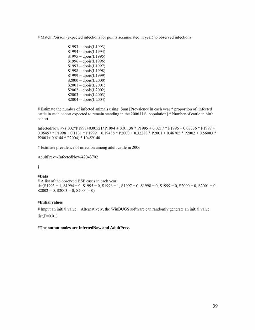
39

# Match Poisson (expected infections for points accumulated in year) to observed infections S1993 ~ dpois(L1993) S1994 ~ dpois(L1994) S1995 ~ dpois(L1995) S1996 ~ dpois(L1996) S1997 ~ dpois(L1997) S1998 ~ dpois(L1998) S1999 ~ dpois(L1999) S2000 ~ dpois(L2000) S2001 ~ dpois(L2001) S2002 ~ dpois(L2002) S2003 ~ dpois(L2003) S2004 ~ dpois(L2004) # Estimate the number of infected animals using; Sum [Prevalence in each year * proportion of infected cattle in each cohort expected to remain standing in the 2006 U.S. population] * Number of cattle in birth cohort InfectedNow <- (.002*P1993+0.00521*P1994 + 0.01138 * P1995 + 0.0217 * P1996 + 0.03736 * P1997 + 0.06457 * P1998 + 0.1131 * P1999 + 0.19488 * P2000 + 0.32288 * P2001 + 0.46705 * P2002 + 0.56003 * P2003+ 0.6144 * P2004) * 10459140 # Estimate prevalence of infection among adult cattle in 2006 AdultPrev<-InfectedNow/42043702 } #Data # A list of the observed BSE cases in each year list(S1993 = 1, S1994 = 0, S1995 = 0, S1996 = 1, S1997 = 0, S1998 = 0, S1999 = 0, S2000 = 0, S2001 = 0, S2002 = 0, S2003 = 0, S2004 = 0)

#Initial values # Imput an initial value. Alternatively, the WinBUGS software can randomly generate an initial value.

list(P=0.01)

#The output nodes are InfectedNow and AdultPrev.

40

Reference List

APHIS (2006). USDA:APHIS: VS, CEAH. Summary of Enhanced BSE Surveillance in the United States, April 28, 2006.

APHIS. (2004) USDA BSE Surveillance Plan: Background on Assumptions and Statistical Inference. APHIS. 2004. 15.

Braun U (1999) Reliability of a diagnosis of BSE made on the basis of clinical signs. The Veterinary Record 145:198-200.

Cannon RM (2002) Demonstrating disease freedom-combining confidence levels. Preventative Veterinary Medicine 52:227-49.

Cockcroft, PD (2000) Clinical sign profile likelihood ratios for bovine spongiform encephalopathy suspects. Research in Veterinary Science 68(3):285-290.

Cohen JT, Duggar K, Gray G, Kreindel S, Abdelrahman H, HabteMariam T, Oryang D, Tameru B. (2001) Evaluation of the Potential for Bovine Spongiform Encephalopathy in the United States. Harvard Center for Risk Analysis/Harvard School of Public Health and Center for Computational Epidemiology, College of Veterinary Medicine, Tuskegee University. November 2001, (revised October 2003). Available at http://www.aphis.usda.gov/lpa/issues/bse/madcow.pdf)

Cohen, J and Gray, G (2004) Comments on USDA bovine spongiform encephalopathy (BSE) surveillance plan. Memorandum to Ron DeHaven, Deputy Administrator, Veterinary Services, APHIS. Harvard Center for Risk Analysis, March 12, 2004.

DEFRA (United Kingdom Department of Environment Food and Rural Affairs) (2005) BSE: Disease control & eradication - The feed ban - Born after the July 1988 ban (BAB) cases. Page last modified 11/22/05 Available November 30, 2005, at: http://www.defra.gov.uk/animalh/bse/controls-eradication/feedban-bornafterban.html

EC (European Commission). (2004) Report on the Monitoring and Testing of Ruminants for the Presence of Transmissible Spongiform Encephalopathy (TSE) in the EU in 2003. http://europa.eu.int/comm/food/food/biosafety/bse/annual_report_tse2003_en.pdf

EC (European Commission). (2005) Report on the Monitoring and Testing of Ruminants for the Presence of Transmissible Spongiform Encephalopathy (TSE) in the EU in 2004. http://europa.eu.int/comm/food/food/biosafety/bse/annual_report_tse2004_en.pdf

EFSA (European Food Safety Authority). (2004) Scientific Report of the European Food Safety Authority on the BSE surveillance model (BSurvE) established by the Community Reference Laboratory for TSE. http://www.efsa.eu.int/science/tse_assessments/bse_tse/661/sr17_bsetse_bsurve_en1.pdf

Evans M, Hastings N, and Peacock B (2000) Statistical Distributions, 2nd ed., John Wiley

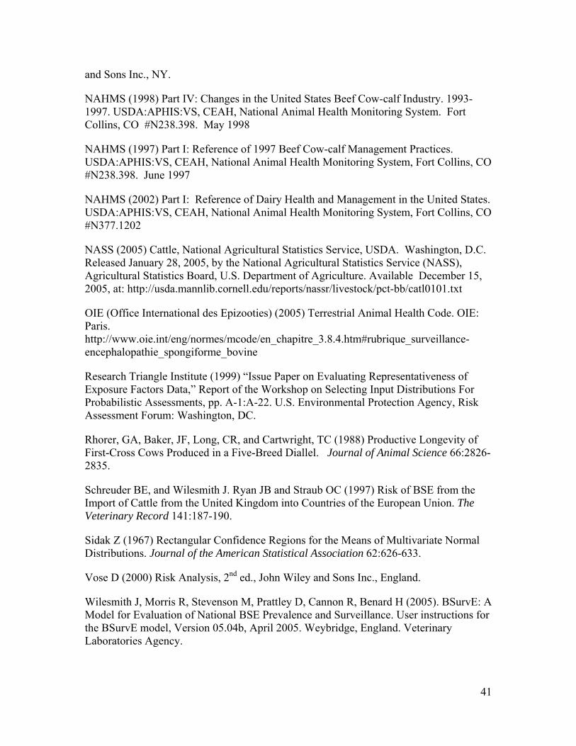
41

and Sons Inc., NY.

NAHMS (1998) Part IV: Changes in the United States Beef Cow-calf Industry. 1993-1997. USDA:APHIS:VS, CEAH, National Animal Health Monitoring System. Fort Collins, CO #N238.398. May 1998

NAHMS (1997) Part I: Reference of 1997 Beef Cow-calf Management Practices. USDA:APHIS:VS, CEAH, National Animal Health Monitoring System, Fort Collins, CO #N238.398. June 1997

NAHMS (2002) Part I: Reference of Dairy Health and Management in the United States. USDA:APHIS:VS, CEAH, National Animal Health Monitoring System, Fort Collins, CO #N377.1202

NASS (2005) Cattle, National Agricultural Statistics Service, USDA. Washington, D.C. Released January 28, 2005, by the National Agricultural Statistics Service (NASS), Agricultural Statistics Board, U.S. Department of Agriculture. Available December 15, 2005, at: http://usda.mannlib.cornell.edu/reports/nassr/livestock/pct-bb/catl0101.txt

OIE (Office International des Epizooties) (2005) Terrestrial Animal Health Code. OIE: Paris. http://www.oie.int/eng/normes/mcode/en_chapitre_3.8.4.htm#rubrique_surveillance-encephalopathie_spongiforme_bovine

Research Triangle Institute (1999) “Issue Paper on Evaluating Representativeness of Exposure Factors Data,” Report of the Workshop on Selecting Input Distributions For Probabilistic Assessments, pp. A-1:A-22. U.S. Environmental Protection Agency, Risk Assessment Forum: Washington, DC.

Rhorer, GA, Baker, JF, Long, CR, and Cartwright, TC (1988) Productive Longevity of First-Cross Cows Produced in a Five-Breed Diallel. Journal of Animal Science 66:2826-2835.

Schreuder BE, and Wilesmith J. Ryan JB and Straub OC (1997) Risk of BSE from the Import of Cattle from the United Kingdom into Countries of the European Union. The Veterinary Record 141:187-190.

Sidak Z (1967) Rectangular Confidence Regions for the Means of Multivariate Normal Distributions. Journal of the American Statistical Association 62:626-633.

Vose D (2000) Risk Analysis, 2nd ed., John Wiley and Sons Inc., England.

Wilesmith J, Morris R, Stevenson M, Prattley D, Cannon R, Benard H (2005). BSurvE: A Model for Evaluation of National BSE Prevalence and Surveillance. User instructions for the BSurvE model, Version 05.04b, April 2005. Weybridge, England. Veterinary Laboratories Agency.

42

Wilesmith J, Morris R, Stevenson M, Cannon R, Prattley D, and Benard H (2004) Development of a Method for the Evaluation of National Surveillance Data and Optimization of National Surveillance Strategies for Bovine Spongiform Encephalopathy. Weybridge, England, European Union TSE Community Reference Laboratory, Veterinary Laboratories Agency.

Wilesmith JW, Ryan JB, and Hueston WD (1992) Bovine spongiform encephalopathy: case-control studies of calf feeding practices and meat and bonemeal inclusion in proprietary concentrates. Research in Veterinary Science 52:325-31.