an equivariant lefschetz fixed-point formula for ... · 4 ivo dell’ambrogio, heath emerson, and...
TRANSCRIPT

arX
iv:1
303.
4777
v1 [
mat
h.K
T]
19
Mar
201
3
AN EQUIVARIANT LEFSCHETZ FIXED-POINT FORMULA
FOR CORRESPONDENCES
IVO DELL’AMBROGIO, HEATH EMERSON, AND RALF MEYER
We dedicate this article to Tamaz Kandelaki, who was a coauthor in an earlier version of this
article, and passed away in 2012. We will remember him for his warm character and his
perseverance in doing mathematics in difficult circumstances.
Abstract. We compute the trace of an endomorphism in equivariant bivari-ant K-theory for a compact group G in several ways: geometrically usinggeometric correspondences, algebraically using localisation, and as a Hattori–Stallings trace. This results in an equivariant version of the classical Lefschetzfixed-point theorem, which applies to arbitrary equivariant correspondences,not just maps.
1. Introduction
Here we continue a series of articles by the last two authors about Euler character-istics and Lefschetz invariants in equivariant bivariant K-theory. These invariantswere introduced in [11,13–16]. The goal is to compute Lefschetz invariants explicitlyin a way that generalises the Lefschetz–Hopf fixed-point formula.
Let X be a smooth compact manifold and f : X → X a self-map with simpleisolated fixed points. The Lefschetz–Hopf fixed-point formula identifies
(1) the sum over the fixed points of f , where each fixed point contributes ±1depending on its index;
(2) the supertrace of the Q-linear, grading-preserving map on K∗(X) ⊗ Q in-duced by f .
It makes no difference in (2) whether we use rational cohomology or K-theorybecause the Chern character is an isomorphism between them.
We will generalise this result in two ways. First, we allow a compact group G toact on X and get elements of the representation ring R(G) instead of numbers. Sec-ondly, we replace self-maps by self-correspondences in the sense of [15]. Sections 2and 3 generalise the invariants (1) and (2) respectively to this setting. The invariantof Section 2 is local and geometric and generalises (1) above; the formulas in Sec-tions 3 and 4 are global and homological and generalise (2) (in two different ways.)The equality of the geometric and homological invariants is our generalisation ofthe Lefschetz fixed-point theorem.
A first step is to interpret the invariants (1) or (2) in a category-theoretic wayin terms of the trace of an endomorphism of a dualisable object in a symmetricmonoidal category.
Let C be a symmetric monoidal category with tensor product ⊗ and tensor unit 1.An object A of C is called dualisable if there is an object A∗, called its dual, and a
2010 Mathematics Subject Classification. 19K99, 19K35, 19D55.This research was supported by the Volkswagen Foundation (Georgian–German non-
commutative partnership). Heath Emerson was supported by a National Science and EngineeringResearch Council of Canada Discovery Grant. Ralf Meyer was supported by the German ResearchFoundation (Deutsche Forschungsgemeinschaft (DFG)) through the Institutional Strategy of theUniversity of Göttingen.
1

2 IVO DELL’AMBROGIO, HEATH EMERSON, AND RALF MEYER
natural isomorphism
C(A⊗B,C) ∼= C(B,A∗ ⊗ C)
for all objects B and C of C. Such duality isomorphisms exist if and only if thereare two morphisms η : 1→ A⊗A∗ and ε : A∗⊗A→ 1, called unit and counit of theduality, that satisfy two appropriate conditions. Let f : A→ A be an endomorphismin C. Then the trace of f is the composite endomorphism
1η−→ A⊗A∗ braid
−−−→ A∗ ⊗AidA∗ ⊗f−−−−−→ A∗ ⊗A
ε−→ 1,
where braid denotes the braiding isomorphism. In this article we also call the tracethe Lefschetz index of the morphism. This is justified by the following example.
Let C be the Kasparov category KK with its usual tensor product structure,A = C(X) for a smooth compact manifold X , and f ∈ KK0(A,A) for some mor-phism. We may construct a dual A∗ from the tangent bundle or the stable normalbundle ofX . In the case of a smooth self-map ofX , and assuming a certain transver-
sality condition, the trace of the morphism f induced by the self-map equals theinvariant (1), that is, equals the number of fixed-points of the map, counted with ap-propriate signs. This is checked by direct computation in Kasparov theory, see [13]for more general results.
This paper springs in part from the reference [13]. A similar invariant to theLefschetz index was introduced there, called the Lefschetz class (of the morphism).The Lefschetz class for an equivariant Kasparov endomorphism of X was defined asan equivariant K-homology class for X . The Lefschetz index, that is, the categoricaltrace, discussed above, is the Atiyah–Singer index of the Lefschetz class of [13].
The main goal of this article is to give a global, homological formula for theLefschetz index generalising the invariant (2) for a non-equivariant self-map. Theformulation and proof of our homological formula works best for Hodgkin Lie groups.A more complicated form applies to all compact groups. The article [13] alsoprovides two formulas for the equivariant Lefschetz class whose equality generalisesthat of the invariants (1) and (2), but the methods there are completely different.
The other main contribution of this article is to compute the geometric expres-
sion for the Lefschetz index in the category kkG
of geometric correspondencesintroduced in [15]. This simplifies the computation in Kasparov’s analytic theoryin [13] and also gives a more general result, since we can work with general smoothcorrespondences rather than just maps. Furthermore, using an idea of Baum andBlock in [4], we give a recipe for composing two smooth equivariant correspondencesunder a weakening of the usual transversality assumption (of [6]). This techniqueis important for computing the Lefschetz index in the case of continuous group ac-tions, where transversality is sometimes difficult to achieve, and in particular, aidsin describing equivariant Euler characteristics in our framework.
Section 2 contains our geometric formula for the Lefschetz index of an equivari-ant self-correspondence. Why is there a nice geometric formula for the Lefschetzindex of a self-map in Kasparov theory? A good explanation is that Connes andSkandalis [6] describe KK-theory for commutative C∗-algebras geometrically, in-cluding the Kasparov product; furthermore, the unit and counit of the KK-dualityfor smooth manifolds have a simple form in this geometric variant of KK. Anequivariant version of the theory in [6] is developed in [15]. In Section 2, we alsorecall some basic results about the geometric KK-theory introduced in [15]. If X is
a smooth compact G-manifold for a compact group G, then KKG∗ (C(X),C(X)) is
isomorphic to the geometrically defined group kkG
∗ (X,X). Its elements are smoothcorrespondences
(1.1) Xb←− (M, ξ)
f−→ X

EQUIVARIANT LEFSCHETZ FIXED-POINT FORMULA 3
consisting of a smooth G-map b, a KG-oriented smooth G-map f , and ξ ∈ K∗G(M).
Theorem 2.18 computes the categorical trace, or Lefschetz index, of such a corre-spondence under suitable assumptions on b and f .
Assume first that X has no boundary and that b and f are transverse; equiva-lently, for allm ∈M with f(m) = b(m) the linear map Db−Df : TmM → Tf(m)Xis surjective. Then
(1.2) Q := {m ∈M | b(m) = f(m)}
is naturally a KG-oriented smooth manifold. We show that the Lefschetz index isthe G-index of the Dirac operator on Q twisted by ξ|Q ∈ K∗
G(Q) (Theorem 2.18).More generally, suppose that the coincidence space Q as defined above is merelyassumed to be a smooth submanifold of M , and that x ∈ TX and Df(ξ) = Db(ξ)implies that ξ ∈ TQ. Then we say that f and b intersect smoothly. For example,the identity correspondence, where f and b are the identity maps on X , does notsatisfy the above transversality hypothesis, but f and b clearly intersect smoothly.In the case of a smooth intersection, the cokernels of the map Df − Db form avector bundle on Q which we call the excess intersection bundle η. This bundlemeasures the failure of transversality of f and b. Let η be KG-oriented. Then TQalso inherits a canonical KG-orientation. The restriction of the Thom class of η tothe zero section gives a class e(η) ∈ K∗
G(Q).Then Theorem 2.18 asserts that the Lefschetz index of the correspondence (1.1)
with smoothly intersecting f and b is the index of the Dirac operator on the coin-cidence manifold Q twisted by ξ ⊗ e(η). This is the main result of Section 2.
In Section 3 we generalise the global homological formula involved in the classicalLefschetz fixed-point theorem, to the equivalent situation. This involves completelydifferent ideas. The basic idea to use Künneth and Universal Coefficient theoremsfor such a formula already appears in [9]. In the equivariant case, these theoremsbecome much more complicated, however. The new idea that we need here is tofirst localise KKG and compute the Lefschetz index in the localisation.
In the introduction, we only state our result in the simpler case of a HodgkinLie group G. Then R(G) is an integral domain and thus embeds into its field
of fractions F . For any G-C∗-algebra A, KG∗ (A) is a Z/2-graded R(G)-module.
Thus KG∗ (A;F ) := KG∗ (A)⊗R(G) F becomes a Z/2-graded F -vector space. Assume
that A is dualisable and belongs to the bootstrap class in KKG. Then KG∗ (A;F )
is finite-dimensional, so that the map on KG∗ (A;F ) induced by an endomorphism
ϕ ∈ KKG0 (A,A) has a well-defined (super)trace in F . Theorem 3.4 asserts thatthis supertrace belongs to R(G) ⊆ F and is equal to the Lefschetz index of ϕ. Inparticular, this applies if A = C(X) for a compact G-manifold.
The results of Sections 2 and 3 together thus prove the following:
Theorem 1.1. Let G be a Hodgkin Lie group, let F be the field of fractions of R(G).
Let X be a closed G-manifold. Let Xb←− (M, ξ)
f−→ X be a smooth G-equivariant
correspondence from X to X with ξ ∈ KdimM−dimXG (X); it represents a class
ϕ ∈ kkG
0 (X,X). Assume that b and f intersect smoothly with KG-oriented ex-
cess intersection bundle η. Equip Q := {m ∈ M | b(m) = f(m)} with its induced
KG-orientation.
Then the R(G)-valued index of the Dirac operator on Q twisted by ξ|Q ⊗ e(η) is
equal to the supertrace of the F -linear map on K∗G(X)⊗R(G) F induced by ϕ.
If G is a connected Lie group, then there is a finite covering G ։ G that is aHodgkin Lie group. We may turnG-actions into G-actions using the projection map,
and get a symmetric monoidal functor KKG → KKG. Since the map R(G)→ R(G)
is clearly injective, we may compute the Lefschetz index of ϕ ∈ KKG0 (A,A) by

4 IVO DELL’AMBROGIO, HEATH EMERSON, AND RALF MEYER
computing instead the Lefschetz index of the image of ϕ in KKG0 (A,A). By the
result mentioned above, this uses the induced map on KG∗ (A) ⊗R(G) F , where F
is the field of fractions of R(G). Thus we get a satisfactory trace formula for allconnected Lie groups. But the result may be quite different from the trace of theinduced map on KG∗ (A)⊗R(G) F .
If G is not connected, then the total ring of fractions of G is a product offinitely many fields. Its factors correspond to conjugacy classes of Cartan subgroupsin G. Each Cartan subgroup H ⊆ G corresponds to a minimal prime ideal pHin R(G). The quotient R(G)/pH is an integral domain and embeds into a field offractions FH . We show that the map R(G) → FH maps the Lefschetz index of ϕ
to the supertrace of KH∗ (ϕ;FH) (Theorem 3.23). It is crucial to use H-equivariantK-theory here. The very simple counterexample 3.7 shows that there may be twoelements ϕ1, ϕ2 ∈ KKG0 (A,A) with different Lefschetz index but inducing the same
map on KG∗ (A).Thus the generalisation of Theorem 1.1 to disconnected G identifies the image
of the index of the Dirac operator on Q twisted by ξ|Q ⊗ e(η) under the canonicalmap R(G) → FH with the supertrace of the FH -linear map on K∗
G(X) ⊗R(G) FHinduced by ϕ, for each Cartan subgroup H .
The trace formulas in Section 3 require the algebra A on which we computethe trace to be dualisable and to belong to an appropriate bootstrap class, namely,the class of all G-C∗-algebras that are KKG-equivalent to a type I G-C∗-algebra.This is strictly larger than the class of G-C∗-algebras that are KKG-equivalentto a commutative one, already if G is the circle group (see [10]). We describethe bootstrap class as being generated by so-called elementary G-C∗-algebras inSection 3.1. This list of generators is rather long, but for the purpose of the tracecomputations, we may localise KKG at the multiplicatively closed subset of non-zero divisors in R(G). The image of the bootstrap class in this localisation has avery simple structure, which is described in Section 3.2. The homological formulafor the Lefschetz index follows easily from this description of the localised bootstrapcategory.
In Section 4, we give a variant of the global homological formula for the tracefor a Hodgkin Lie group G. Given a commutative ring R and an R-module Mwith a projective resolution of finite type, we may define a Hattori–Stallings tracefor endomorphisms of M by lifting the endomorphism to a finite type projectiveresolution and using the standard trace for endomorphisms of finitely generatedprojective resolutions. This defines the trace of the R(G)-module homomorphism
KG∗ (ϕ) : KG∗ (A)→ KG∗ (A) in R(G) without passing through a field of fractions.
2. Lefschetz indices in geometric bivariant K-theory
The category kkGintroduced in [15] provides a geometric analogue of Kasparov
theory. We first recall some basic facts about this category and duality in bivariantK-theory from [14–16] and then compute Lefschetz indices in it as intersectionproducts. Later we are going to compare this with other formulas for Lefschetzindices. We also prove an excess intersection formula to compute the compositionof geometric correspondences under a weaker assumption than transversality. Thisformula goes back to Baum and Block [4].
All results in this section extend to the case where G is a proper Lie groupoidwith enough G-vector bundles in the sense of [14, Definition 3.1] because the theoryin [14–16] is already developed in this generality. For the sake of concreteness, welimit our treatment here to compact Lie groups acting on smooth manifolds.

EQUIVARIANT LEFSCHETZ FIXED-POINT FORMULA 5
The results in this section work both for real and complex K-theory. For concrete-ness, we assume in our notation that we are dealing with the complex case. In thereal case, K must be replaced by KO throughout. In particular, KG-orientations(that is, G-equivariant Spinc-structures) must be replaced by KOG-orientations(that is, G-equivariant Spin structures). In some examples, we use the isomorphisms
kkG
2n(pt, pt) = R(G) and kkG
2n+1(pt, pt) = 0 for all n ∈ Z. Here R(G) denotes therepresentation ring of G. Of course, this is true only in complex K-theory.
2.1. Geometric bivariant K-theory. Like Kasparov theory, geometric bivari-
ant K-theory yields a category kkG. Its objects are (Hausdorff) locally compact
G-spaces; arrows from X to Y are geometric correspondences from X to Y in thesense of [15, Definition 2.3]. These consist of
M : a G-space;b: a G-map (that is, a continuous G-equivariant map) b : M → X ;ξ: a G-equivariant K-theory class on M with X-compact support (where we
view M as a space over X via the map b); we write ξ ∈ RK∗G,X(M);
f : a KG-oriented normally non-singular G-map f : M → Y .
Equivariant K-theory with X-compact support and equivariant vector bundles aredefined in [12, Definitions 2.5 and 2.6]. If b is a proper map, in particular if Mis compact, then RK∗
G,X(M) is the ordinary G-equivariant (compactly supported)
K-theory K∗G(M) of M .
A KG-oriented normally non-singular map from M to Y consists of
V : a KG-oriented G-vector bundle on M ,E: a KG-oriented finite-dimensional linear G-representation, giving rise to a
trivial KG-oriented G-vector bundle Y × E on Y ,
f : a G-equivariant homeomorphism from the total space of V to an open
subset in the total space of Y × E, f : V → Y × E.
We will not distinguish between a vector bundle and its total space in our notation.
A normally non-singular map f = (V,E, f) has an underlying map
M Vf−→ Y × E ։ Y,
where the first map is the zero section of the vector bundle V and the third mapis the coordinate projection. This map is called its “trace” in [14], but we avoidthis name here because we use “trace” in a different sense. The degree of f isd = dim V − dimE. A wrong-way element f! ∈ KKGd (C0(M),C0(Y )) induced by fis defined in [14, Section 5.3]).
Our geometric correspondences are variants of those introduced by Alain Connesand Georges Skandalis in [6]. The changes in the definition avoid technical problemswith the usual definition in the equivariant case.
The (Z/2-graded) geometric KK-group kkG
∗ (X,Y ) is defined as the quotientof the set of geometric correspondences from X to Y by an appropriate equiva-lence relation, generated by bordism, Thom modification, and equivalence of nor-mally non-singular maps. Bordism includes homotopies for the maps b and f by[15, Lemma 2.12]. We will use this several times below. The Thom modification al-lows to replace the spaceM by the total space of a KG-oriented vector bundle onM .In particular, we could take the KG-oriented vector bundle from the normally non-singular map f . This results in an equivalent normally non-singular map wheref : M → Y is a special submersion, that is, an open embedding followed by a coor-dinate projection Y ×E ։ Y for some linear G-representation E. Correspondenceswith this property are called special.

6 IVO DELL’AMBROGIO, HEATH EMERSON, AND RALF MEYER
The composition in kkGis defined as an intersection product (see Section 2.2) if
the map f : M → Y is such a special submersion. This turns kkG
into a category;the identity map on X is the correspondence with f = b = idX and ξ = 1. The
product of G-spaces provides a symmetric monoidal structure in kkG
(see [15,Theorem 2.27]).
There is an additive, grading-preserving, symmetric monoidal functor
kkG
∗ (X,Y )→ KKG∗ (C0(X),C0(Y )).
This is an isomorphism if X is normally non-singular by [15, Corollary 4.3], thatis, if there is a normally non-singular map X → pt. This means that there is aG-vector bundle V over X whose total space is G-equivariantly homeomorphic toan open G-invariant subset of some linear G-space. In particular, by Mostow’sEmbedding Theorem smooth G-manifolds of finite orbit type are normally non-singular (see [14, Theorem 3.22]).
Stable KG-orientations play an important technical role in our trace formulas andshould therefore be treated with care. A KG-orientation on a G-vector bundle Vis, by definition, a G-equivariant complex spinor bundle for V . (This is equivalentto a reduction of the structure group to Spinc.) Given such KG-orientations on V1
and V2, we get an induced KG-orientation on V1 ⊕ V2; conversely, KG-orientationson V1 ⊕ V2 and V1 induce one on V2.
Let ξ ∈ RK0G(M) be represented by the formal difference [V1] − [V2] of two
G-vector bundles. A stable KG-orientation on ξ means that we are given anotherG-vector bundle V3 and KG-orientations on both V1 ⊕ V3 and V2 ⊕ V3. Sinceξ = [V1⊕V3]− [V2⊕V3], this implies that ξ is a formal difference of two KG-orientedG-vector bundles. Conversely, assume that ξ = [W1]− [W2] with two KG-orientedG-vector bundles; then there are G-vector bundles V3 and W3 such that Vi ⊕ V3
∼=Wi⊕W3 for i = 1, 2; sinceW3 is a direct summand in a KG-orientedG-vector bundle,we may enlarge V3 andW3 so thatW3 itself is KG-oriented. Then Vi⊕V3
∼=Wi⊕W3
for i = 1, 2 inherit KG-orientations. Roughly speaking, stably KG-oriented K-theoryclasses are equivalent to formal differences of KG-oriented G-vector bundles.
A KG-orientation on a normally non-singular map f = (V,E, f) from M to Ymeans that both V and E are KG-oriented. Since “lifting” allows us to replace E byE⊕E′ and V by V ⊕ (M ×E′), we may assume without loss of generality that E isalready KG-oriented. Thus a KG-orientation on f becomes equivalent to one on V .But the chosen KG-orientation on E remains part of the data: changing it changesthe KG-orientation on f . By [14, Lemma 5.13], all essential information is containedin a KG-orientation on the formal difference [V ]− [M × E] ∈ RK0
G(M), which wecall the stable normal bundle of the normally non-singular map f . If [V ]− [M ×E]is KG-oriented, then we may find a G-vector bundle V3 such that V ⊕V3 and (M ×E)⊕V3 are KG-oriented. Since (M ×E)⊕V3 is a direct summand in a KG-orientedtrivial G-vector bundle, we may assume without loss of generality that V3 itself istrivial, V3 = M × E′, and that already E ⊕ E′ is KG-oriented. Lifting f along E′
then gives a normally non-singular map (V ⊕ (M × E′), E ⊕ E′, f × idE′), whereboth V ⊕ (M × E′) and E ⊕ E′ are KG-oriented. Thus a KG-orientation on f isequivalent to a stable KG-orientation on the stable normal bundle of f .
Lemma 2.1. If f = (V,E, f) is a smooth normally non-singular map with under-
lying map f : M → Y , then its stable normal bundle is equal to f∗[TY ] − [TM ] ∈RK0
G(M).
Proof. The tangent bundles of the total spaces of V and Y × E are TM ⊕ V andTY ⊕E, respectively. Since f is an open embedding, f∗(TY ⊕E) ∼= TM ⊕V . This
implies f∗(TY )⊕ (M ×E) ∼= TM ⊕V . Thus [V ]− [M ×E] = f∗[TY ]− [TM ]. �
EQUIVARIANT LEFSCHETZ FIXED-POINT FORMULA 7
This lemma also shows that the stable normal bundle of f and hence the ori-entability assumption depend only on the equivalence class of f .
Another equivalent way to describe stable KG-orientations is the following. Sup-pose we are already given aG-vector bundleW on Y such that TY⊕V is KG-oriented.Then a stable KG-orientation on f is equivalent to one on
[f∗V ⊕ TM ] = f∗[TY ⊕ V ]− (f∗[TY ]− [TM ]),
which is equivalent to a KG-orientation on f∗V ⊕ TM in the usual sense.If X and Y are smooth G-manifolds (without boundary), we may require the
maps b and f and the vector bundles V and E to be smooth. This leads to a smooth
variant of kkG. This variant is isomorphic to the one defined above by [15, Theorem
4.8] provided X is of finite orbit type and hence normally non-singular.Working in the smooth setting has two advantages.First, assuming M to be of finite orbit type, [14, Theorem 3.22] shows that any
smooth G-map f : M → Y lifts to a smooth normally non-singular map that isunique up to equivalence. Thus we may replace normally non-singular maps bysmooth maps in the usual sense in the definition of a geometric correspondence.Moreover, Nf = f∗[TY ] − [TM ], so f is KG-oriented if and only if there areKG-oriented G-vector bundles V1 and V2 over M with f∗[TY ] ⊕ V1
∼= TM ⊕ V2
(compare [14, Corollary 5.15]).Secondly, in the smooth setting there is a particularly elegant way of composing
correspondences when they satisfy a suitable transversality condition, see [15, Corol-lary 2.39]. This description of the composition is due to Connes and Skandalis [6].
2.2. Composition of geometric correspondences. By [15, Theorem 2.38], asmooth normally non-singular map lifting f : M1 → Y and a smooth map b : M2 →Y are transverse if
Dm1f(Tm1
M1) +Dm2b(Tm2
M2) = TyY
for all m1 ∈M1, m2 ∈M2 with y := f(m1) = b(m2). Equivalently, the map
Df −Db : pr∗1(TM1)⊕ pr∗
2(TM2)→ (f ◦ pr1)∗(TY )
is surjective; this is a bundle map of vector bundles over
M1 ×Y M2 := {(m1,m2) | f(m1) = b(m2)},
where pr1 : M1 ×Y M2 → M1 and pr2 : M1 ×Y M2 → M2 denote the restrictionsto M1 ×Y M2 of the coordinate projections. (We shall always use this notation forrestrictions of coordinate projections.)
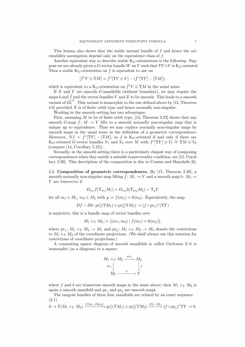
A commuting square diagram of smooth manifolds is called Cartesian if it isisomorphic (as a diagram) to a square
M1 ×Y M2 M2
M1 Y
pr2
pr1 f
b
where f and b are transverse smooth maps in the sense above; then M1 ×Y M2 isagain a smooth manifold and pr1 and pr2 are smooth maps.
The tangent bundles of these four manifolds are related by an exact sequence(2.1)
0→ T(M1 ×Y M2)(Dpr
1,Dpr
2)
−−−−−−−−→ pr∗1(TM1)⊕ pr∗
2(TM2)Df−Db−−−−−→ (f ◦ pr1)
∗TY → 0.
8 IVO DELL’AMBROGIO, HEATH EMERSON, AND RALF MEYER
That is, T(M1 ×Y M2) is the sub-bundle of pr∗1(TM1) ⊕ pr∗
2(TM2) consisting ofthose vectors (m1, ξ,m2, η) ∈ TM1⊕TM2 (where f(m1) = b(m2)) with Dm1
f(ξ) =Dm2
b(η). We may denote this bundle briefly by TM1 ⊕TY TM2.Furthermore, from (2.1),
(2.2) T(M1 ×Y M2)− pr∗2(TM2) = pr∗
1(TM1 − f∗(TY ))
as stable G-vector bundles. Thus a stable KG-orientation for TM1−f∗(TY ) may bepulled back to one for T(M1×YM2)−pr∗
2(TM2). More succinctly, a KG-orientationfor the map f induces one for pr2.
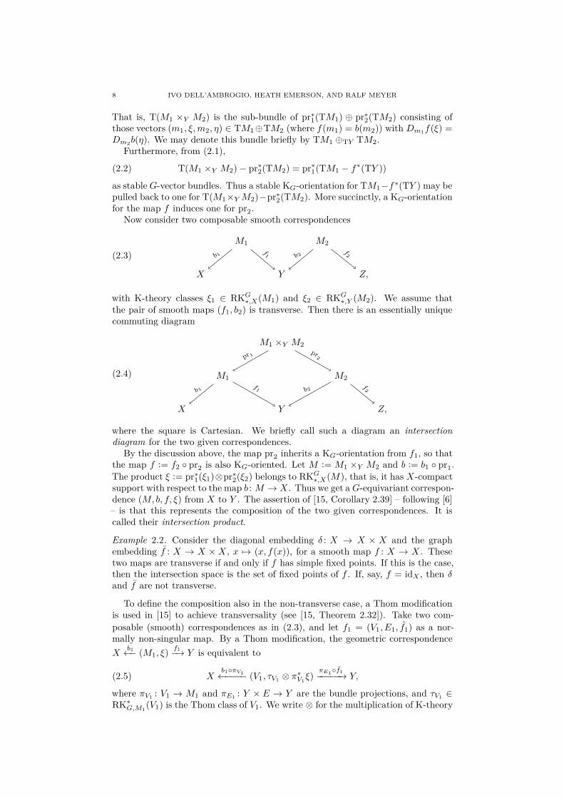
Now consider two composable smooth correspondences
(2.3)
M1 M2
X Y Z,
b1f1 b2
f2
with K-theory classes ξ1 ∈ RKG∗,X(M1) and ξ2 ∈ RKG∗,Y (M2). We assume thatthe pair of smooth maps (f1, b2) is transverse. Then there is an essentially uniquecommuting diagram
(2.4)
M1 ×Y M2
M1 M2
X Y Z,
pr 1pr
2
b1f
1 b2f2
where the square is Cartesian. We briefly call such a diagram an intersection
diagram for the two given correspondences.By the discussion above, the map pr2 inherits a KG-orientation from f1, so that
the map f := f2 ◦ pr2 is also KG-oriented. Let M := M1 ×Y M2 and b := b1 ◦ pr1.
The product ξ := pr∗1(ξ1)⊗pr∗
2(ξ2) belongs to RKG∗,X(M), that is, it has X-compactsupport with respect to the map b : M → X . Thus we get aG-equivariant correspon-dence (M, b, f, ξ) from X to Y . The assertion of [15, Corollary 2.39] – following [6]– is that this represents the composition of the two given correspondences. It iscalled their intersection product.
Example 2.2. Consider the diagonal embedding δ : X → X × X and the graphembedding f : X → X ×X , x 7→ (x, f(x)), for a smooth map f : X → X . Thesetwo maps are transverse if and only if f has simple fixed points. If this is the case,then the intersection space is the set of fixed points of f . If, say, f = idX , then δand f are not transverse.
To define the composition also in the non-transverse case, a Thom modificationis used in [15] to achieve transversality (see [15, Theorem 2.32]). Take two com-
posable (smooth) correspondences as in (2.3), and let f1 = (V1, E1, f1) as a nor-mally non-singular map. By a Thom modification, the geometric correspondence
Xb1←− (M1, ξ)
f1
−→ Y is equivalent to
(2.5) Xb1◦πV1←−−−− (V1, τV1
⊗ π∗V1ξ)
πE1◦f1
−−−−−→ Y,
where πV1: V1 → M1 and πE1
: Y × E → Y are the bundle projections, and τV1∈
RK∗G,M1
(V1) is the Thom class of V1. We write ⊗ for the multiplication of K-theory

EQUIVARIANT LEFSCHETZ FIXED-POINT FORMULA 9
classes. The support of such a product is the intersection of the supports of thefactors. Hence the support of τV1
⊗ π∗V1ξ is an X-compact subset of V1.
The forward map V1 → Y in (2.5) is a special submersion and, in particular,a submersion. As such it is transverse to any other map b2 : M2 → Y . Henceafter the Thom modification we may compute the composition of correspondencesas an intersection product of the correspondence (2.5) with the correspondence
Yb2←−M2
f2
−→ Y . This yields
(2.6) Xb1◦πV1
◦pr1
←−−−−−−−(V1 ×Y M2, pr
∗V1(τV1⊗ π∗
V1(ξ))
) f2◦pr2−−−−→ Z,
where
V1 ×Y M2 := {(x, v,m2) ∈ V1 ×M2 | (πE1◦ f1)(x, v) = b2(m2)}
and pr1 : V1 ×Y M2 → V1 and pr2 : V1 ×Y M2 →M2 are the coordinate projections.The intersection space V1 ×Y M2 is a smooth manifold with tangent bundle
TV1 ⊕TY TM2 := pr∗1(TV1)⊕(πE1
◦f1)∗(TY ) pr∗2(TM2),
and the map pr2 is a submersion with fibres tangent to E1. Thus it is KG-oriented.This recipe to define the composition product for all geometric correspondences
is introduced in [15]. It is shown there that it is equivalent to the intersectionproduct if f1 and b2 are transverse. But the space V1 ×Y M2 has high dimension,making it inefficient to compute with this formula. And we are usually given onlythe underlying map f1 : M1 → Y , not its factorisation as a normally non-singularmap – and the latter is difficult to compute. We will weaken the transversalityrequirement in Section 2.5. The more general condition still applies, say, if f1 = b2.This is particularly useful for computing Euler characteristics.
2.3. Duality and the Lefschetz index. Duality plays a crucial role in [15] inorder to compare the geometric and analytic models of equivariant Kasparov theory.Duality is also used in [16, Definition 4.26] to construct a Lefschetz map
(2.7) L : KKG∗(C(X),C(X)
)→ KKG∗ (C(X),C),
for a compact smooth G-manifold X . We may compose L with the index mapKKG∗ (C(X),C) → KKG∗ (C,C) ∼= R(G) to get a Lefschetz index L-ind(f) ∈ R(G)
for any f ∈ KKG∗(C(X),C(X)
). This is the invariant we will be studying in this
paper.This Lefschetz map L is a special case of a very general construction. Let C be
a symmetric monoidal category. Let A be a dualisable object of C with a dual A∗.Let η : 1 → A ⊗ A∗ and ε : A∗ ⊗ A → 1 be the unit and counit of the duality.Being unit and counit of a duality means that they satisfy the zigzag equations:the composition
(2.8) Aη⊗idA−−−−→ A⊗A∗ ⊗A
idA⊗ε−−−−→ A
is equal to the identity idA : A→ A, and similarly for the composition
(2.9) A∗ idA∗ ⊗η−−−−−→ A∗ ⊗A⊗A∗ ε⊗idA∗
−−−−−→ A∗.
If C is Z-graded, then we may allow dualities to shift degrees. Then some signs arenecessary in the zigzag equations, see [16, Theorem 5.5].
Given a multiplication map m : A⊗A→ A, we define the Lefschetz map
L : C(A,A)→ C(A,1)
by sending an endomorphism f : A→ A to the composite morphism
A ∼= A⊗ 1idA⊗η−−−−→ A⊗A⊗A∗ m⊗idA∗
−−−−−→ A⊗A∗ f⊗idA∗
−−−−−→ A⊗A∗ braid−−−→ A∗ ⊗A
ε−→ 1.
10 IVO DELL’AMBROGIO, HEATH EMERSON, AND RALF MEYER
This depends only on m and f , not on the choices of the dual, unit and counit. Forf = idA we get the higher Euler characteristic of A in C(A,1).
While the geometric computations below give the Lefschetz map as defined above,the global homological computations in Sections 3 and 4 only apply to the followingcoarser invariant:
Definition 2.3. The Lefschetz index L-ind(f) (or trace tr(f)) of an endomorphismf : A→ A is the composite
(2.10) 1η−→ A⊗A∗ braid
−−−→ A∗ ⊗AidA∗ ⊗f−−−−−→ A∗ ⊗A
ε−→ 1,
where braid denotes the braiding. The Lefschetz index of idA is called the Euler
characteristic of A.
If A is a unital algebra object in C with multiplication m : A⊗A→ A and unitu : 1 → A, then L-ind(f) = L(f) ◦ u. In particular, the Euler characteristic is thecomposite of the higher Euler characteristic with u.
In this section, we work in C = kkG
for a compact group G with 1 = pt and⊗ = ×. In Section 3, we work in the related analytic category C = KKG with1 = C and the usual tensor product.
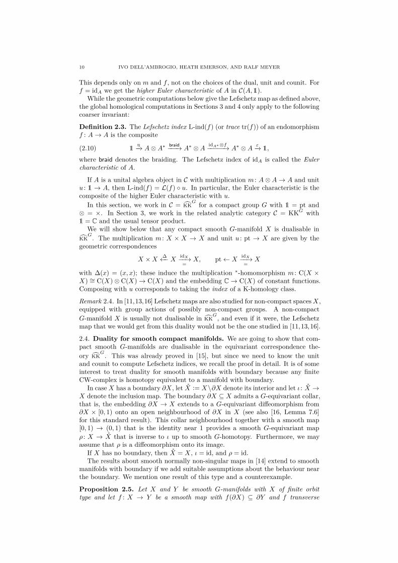
We will show below that any compact smooth G-manifold X is dualisable in
kkG. The multiplication m : X × X → X and unit u : pt → X are given by the
geometric correspondences
X ×X∆←− X
idX−−→=
X, pt← XidX−−→=
X
with ∆(x) = (x, x); these induce the multiplication ∗-homomorphism m : C(X ×X) ∼= C(X)⊗ C(X)→ C(X) and the embedding C→ C(X) of constant functions.Composing with u corresponds to taking the index of a K-homology class.
Remark 2.4. In [11,13,16] Lefschetz maps are also studied for non-compact spacesX ,equipped with group actions of possibly non-compact groups. A non-compact
G-manifold X is usually not dualisable in kkG, and even if it were, the Lefschetz
map that we would get from this duality would not be the one studied in [11,13,16].
2.4. Duality for smooth compact manifolds. We are going to show that com-pact smooth G-manifolds are dualisable in the equivariant correspondence the-
ory kkG. This was already proved in [15], but since we need to know the unit
and counit to compute Lefschetz indices, we recall the proof in detail. It is of someinterest to treat duality for smooth manifolds with boundary because any finiteCW-complex is homotopy equivalent to a manifold with boundary.
In caseX has a boundary ∂X , let X := X\∂X denote its interior and let ι : X →X denote the inclusion map. The boundary ∂X ⊆ X admits a G-equivariant collar,that is, the embedding ∂X → X extends to a G-equivariant diffeomorphism from∂X × [0, 1) onto an open neighbourhood of ∂X in X (see also [16, Lemma 7.6]for this standard result). This collar neighbourhood together with a smooth map[0, 1) → (0, 1) that is the identity near 1 provides a smooth G-equivariant map
ρ : X → X that is inverse to ι up to smooth G-homotopy. Furthermore, we mayassume that ρ is a diffeomorphism onto its image.
If X has no boundary, then X = X , ι = id, and ρ = id.The results about smooth normally non-singular maps in [14] extend to smooth
manifolds with boundary if we add suitable assumptions about the behaviour nearthe boundary. We mention one result of this type and a counterexample.
Proposition 2.5. Let X and Y be smooth G-manifolds with X of finite orbit
type and let f : X → Y be a smooth map with f(∂X) ⊆ ∂Y and f transverse

EQUIVARIANT LEFSCHETZ FIXED-POINT FORMULA 11
to ∂Y . Then f lifts to a normally non-singular map, and any two such normally
non-singular liftings of f are equivalent.
Proof. Since X has finite orbit type, we may smoothly embed X into a finite-dimensional linear G-representation E. Our assumptions ensure that the resultingmap X → Y × E is a smooth embedding between G-manifolds with boundaryin the sense of [14, Definition 3.17] and hence has a tubular neighbourhood by[14, Theorem 3.18]. This provides a normally non-singular map X → Y lifting f .The uniqueness up to equivalence is proved as in the proof of [14, Theorem 4.36]. �
Example 2.6. The inclusion map {0} → [0, 1) is a smooth map between manifoldswith boundary, but it does not lift to a smooth normally non-singular map.
Let X be a smooth compact G-manifold. Since X has finite orbit type, it embedsinto some linear G-representation E. We may choose this G-representation to beKG-oriented and even-dimensional by a further stabilisation. Let NX ։ X bethe normal bundle for such an embedding X → E. Thus TX ⊕ NX ∼= X × E isG-equivariantly isomorphic to a KG-oriented trivial G-vector bundle.
Theorem 2.7. Let X be a smooth compact G-manifold, possibly with boundary.
Then X is dualisable in kkG
∗ with dual NX, and the unit and counit for the duality
are the geometric correspondences
pt← X(id,ζρ)−−−−→ X ×NX, NX ×X
(id,ιπ)←−−−− NX → pt,
where ζ : X → NX is the zero section, ρ : X → X is some G-equivariant collar
retraction, π : NX → X is the bundle projection, and ι : X → X the identical
inclusion. The K-theory classes on the space in the middle are the trivial rank-one
vector bundles for both correspondences.
Proof. First we must check that the purported unit and counit above are indeedgeometric correspondences; this contains describing the KG-orientations on theforward maps, which is part of the data of the geometric correspondences.
The maps X → pt and NX → NX × X above are proper. Hence there isno support restriction for the K-theory class on the middle space, and the trivialrank-one vector bundle is allowed.
By the Tubular Neighbourhood Theorem, the normal bundle NX of the em-bedding X → E is diffeomorphic to an open subset of E. This gives a canonicalisomorphism between the tangent bundle of NX and E. We choose this isomor-phism and the given KG-orientation on the linear G-representation E to KG-orientNX and thus the projection NX → pt. With this KG-orientation, the counit
NX × X(id,ιπ)←−−−− NX → pt is a G-equivariant geometric correspondence – even a
special one in the sense of [15].
We identify the tangent bundle of X ×NX with TX ×TX ⊕NX in the obviousway. The normal bundle of the embedding (id, ζρ) : X → X ×NX is isomorphic to
the quotient of TX⊕ρ∗(TX)⊕ρ∗(NX) by the relation (ξ,Dρ(ξ), 0) ∼ 0 for ξ ∈ TX .We identify this with TX⊕NX ∼= X×E by (ξ1, ξ2, η) 7→ (Dρ−1(ξ2)− ξ1, Dρ
−1(η))
for ξ1 ∈ TxX , ξ2 ∈ Tρ(x)X , η ∈ ρ∗(NX)x = Nρ(x)X . With this KG-orientation on(id, ζρ), the unit above is a G-equivariant geometric correspondence. A boundaryof X , if present, causes no problems here. The same goes for the computationsbelow: although the results in [15] are formulated for smooth manifolds withoutboundary, they continue to hold in the cases we need.
We establish the duality isomorphism by checking the zigzag equations as in[16, Theorem 5.5]. This amounts to composing geometric correspondences. In thecase at hand, the correspondences we want to compose are transverse, so that they
12 IVO DELL’AMBROGIO, HEATH EMERSON, AND RALF MEYER
may be composed by intersections as in Section 2.2. Actually, we are dealing withmanifolds with boundary, but the argument goes through nevertheless. We writedown the diagrams together with the relevant Cartesian square.
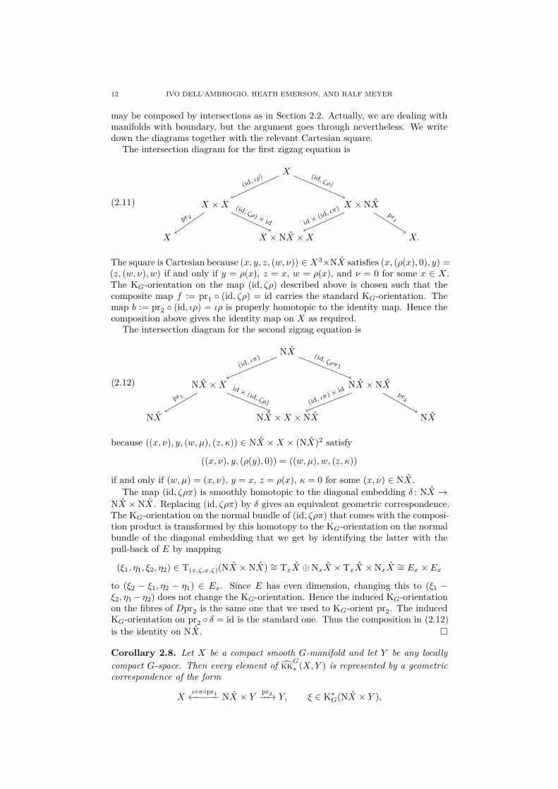
The intersection diagram for the first zigzag equation is
(2.11)
X
X ×X X ×NX
X X ×NX ×X X.
(id, ιρ
) (id, ζρ)
pr 2
(id, ζρ) × id id × (id, ιπ
)pr
1
The square is Cartesian because (x, y, z, (w, ν)) ∈ X3×NX satisfies (x, (ρ(x), 0), y) =(z, (w, ν), w) if and only if y = ρ(x), z = x, w = ρ(x), and ν = 0 for some x ∈ X .The KG-orientation on the map (id, ζρ) described above is chosen such that thecomposite map f := pr1 ◦ (id, ζρ) = id carries the standard KG-orientation. Themap b := pr2 ◦ (id, ιρ) = ιρ is properly homotopic to the identity map. Hence thecomposition above gives the identity map on X as required.
The intersection diagram for the second zigzag equation is
(2.12)
NX
NX ×X NX ×NX
NX NX ×X ×NX NX
(id, ιπ
) (id, ζρπ)
pr 1
id × (id, ζρ) (id, ιπ
) × id pr2
because ((x, ν), y, (w, µ), (z, κ)) ∈ NX ×X × (NX)2 satisfy
((x, ν), y, (ρ(y), 0)) = ((w, µ), w, (z, κ))
if and only if (w, µ) = (x, ν), y = x, z = ρ(x), κ = 0 for some (x, ν) ∈ NX.
The map (id, ζρπ) is smoothly homotopic to the diagonal embedding δ : NX →
NX ×NX . Replacing (id, ζρπ) by δ gives an equivalent geometric correspondence.The KG-orientation on the normal bundle of (id, ζρπ) that comes with the composi-tion product is transformed by this homotopy to the KG-orientation on the normalbundle of the diagonal embedding that we get by identifying the latter with thepull-back of E by mapping
(ξ1, η1, ξ2, η2) ∈ T(x,ζ,x,ζ)(NX × NX) ∼= TxX ⊕NxX × TxX ×NxX ∼= Ex × Ex
to (ξ2 − ξ1, η2 − η1) ∈ Ex. Since E has even dimension, changing this to (ξ1 −ξ2, η1− η2) does not change the KG-orientation. Hence the induced KG-orientationon the fibres of Dpr2 is the same one that we used to KG-orient pr2. The inducedKG-orientation on pr2 ◦ δ = id is the standard one. Thus the composition in (2.12)
is the identity on NX. �
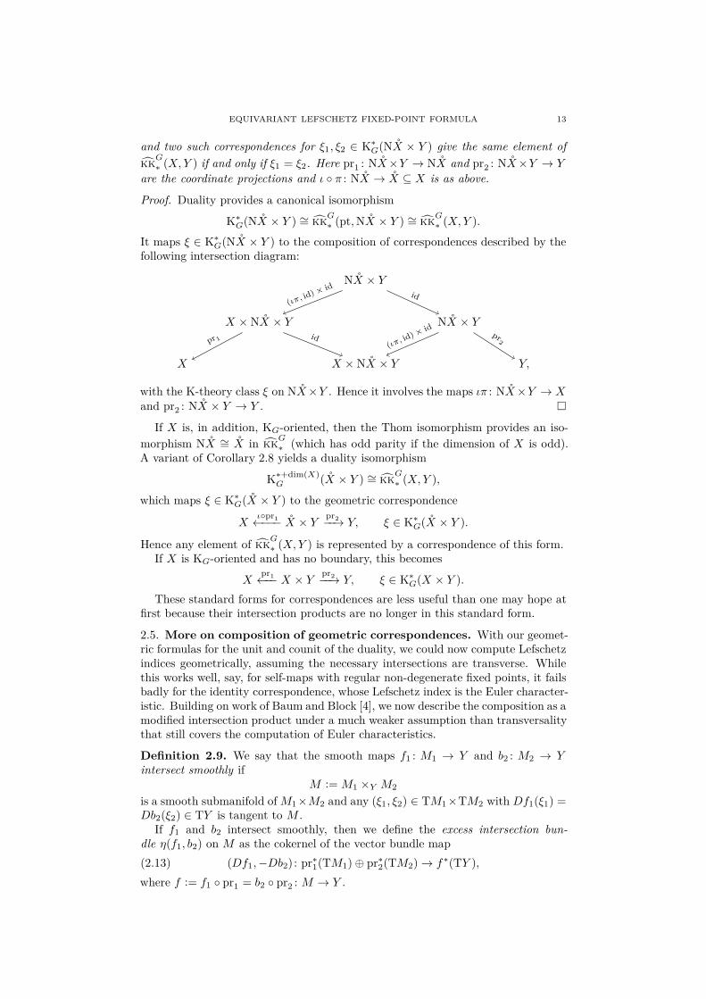
Corollary 2.8. Let X be a compact smooth G-manifold and let Y be any locally
compact G-space. Then every element of kkG
∗ (X,Y ) is represented by a geometric
correspondence of the form
Xι◦π◦pr
1←−−−−− NX × Ypr
2−−→ Y, ξ ∈ K∗G(NX × Y ),
EQUIVARIANT LEFSCHETZ FIXED-POINT FORMULA 13
and two such correspondences for ξ1, ξ2 ∈ K∗G(NX × Y ) give the same element of
kkG
∗ (X,Y ) if and only if ξ1 = ξ2. Here pr1 : NX×Y → NX and pr2 : NX×Y → Y
are the coordinate projections and ι ◦ π : NX → X ⊆ X is as above.
Proof. Duality provides a canonical isomorphism
K∗G(NX × Y ) ∼= kk
G
∗ (pt,NX × Y ) ∼= kkG
∗ (X,Y ).
It maps ξ ∈ K∗G(NX × Y ) to the composition of correspondences described by the
following intersection diagram:
NX × Y
X ×NX × Y NX × Y
X X × NX × Y Y,
(ιπ, id
) × idid
pr 1id
(ιπ, id
) × idpr
2
with the K-theory class ξ on NX×Y . Hence it involves the maps ιπ : NX×Y → Xand pr2 : NX × Y → Y . �
If X is, in addition, KG-oriented, then the Thom isomorphism provides an iso-
morphism NX ∼= X in kkG
∗ (which has odd parity if the dimension of X is odd).A variant of Corollary 2.8 yields a duality isomorphism
K∗+dim(X)G (X × Y ) ∼= kk
G
∗ (X,Y ),
which maps ξ ∈ K∗G(X × Y ) to the geometric correspondence
Xι◦pr
1←−−− X × Ypr
2−−→ Y, ξ ∈ K∗G(X × Y ).
Hence any element of kkG
∗ (X,Y ) is represented by a correspondence of this form.If X is KG-oriented and has no boundary, this becomes
Xpr
1←−− X × Ypr
2−−→ Y, ξ ∈ K∗G(X × Y ).
These standard forms for correspondences are less useful than one may hope atfirst because their intersection products are no longer in this standard form.
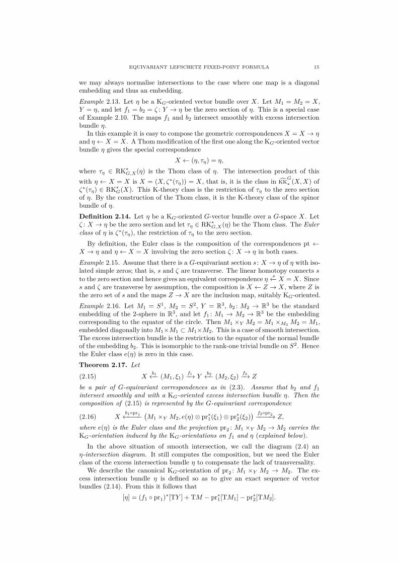
2.5. More on composition of geometric correspondences. With our geomet-ric formulas for the unit and counit of the duality, we could now compute Lefschetzindices geometrically, assuming the necessary intersections are transverse. Whilethis works well, say, for self-maps with regular non-degenerate fixed points, it failsbadly for the identity correspondence, whose Lefschetz index is the Euler character-istic. Building on work of Baum and Block [4], we now describe the composition as amodified intersection product under a much weaker assumption than transversalitythat still covers the computation of Euler characteristics.
Definition 2.9. We say that the smooth maps f1 : M1 → Y and b2 : M2 → Yintersect smoothly if
M :=M1 ×Y M2
is a smooth submanifold ofM1×M2 and any (ξ1, ξ2) ∈ TM1×TM2 with Df1(ξ1) =Db2(ξ2) ∈ TY is tangent to M .
If f1 and b2 intersect smoothly, then we define the excess intersection bun-
dle η(f1, b2) on M as the cokernel of the vector bundle map
(2.13) (Df1,−Db2) : pr∗1(TM1)⊕ pr∗
2(TM2)→ f∗(TY ),
where f := f1 ◦ pr1 = b2 ◦ pr2 : M → Y .

14 IVO DELL’AMBROGIO, HEATH EMERSON, AND RALF MEYER
If the maps f1 and b2 are G-equivariant with respect to a compact group G, thenthe excess intersection bundle is a G-vector bundle.
We call the square
M M2
M1 Y
pr2
pr1 f1
b2
η-Cartesian if f1 and b2 intersect smoothly with excess intersection bundle η.
If M is a smooth submanifold of M1 ×M2, then TM ⊆ T(M1 ×M2); and if(ξ1, ξ2) ∈ T(M1 ×M2) is tangent to M , then Df1(ξ1) = Db2(ξ2) in TY . Thesepairs (ξ1, ξ2) form a subspace of T(M1 ×M2)|M = pr∗
1TM1 ⊕ pr∗2TM2, which in
general need not be a vector bundle, that is, its rank need not be locally constant.The smooth intersection assumption forces it to be a subbundle: the kernel of themap in (2.13). Hence the excess intersection bundle is a vector bundle overM , andthere is the following exact sequence of vector bundles over M :
(2.14) 0→ TM → pr∗1(TM1)⊕ pr∗
2(TM2)(Df1,−Db2)−−−−−−−−→ (f1 ◦ pr1)
∗(TY )→ η → 0.
Example 2.10. Let M1 = M2 = X and let f1 = b2 = i : X → Y be an injectiveimmersion. Then M1 ×Y M2
∼= X is the diagonal in M1 × M2 = X2, which isa smooth submanifold. Furthermore, if (ξ1, ξ2) ∈ TM1 × TM2 satisfy Df1(ξ1) =Db2(ξ2), then ξ1 = ξ2 because Di : TM → TY is assumed injective. Hence M1
andM2 intersect smoothly, and the excess intersection bundle is the normal bundleof the immersion i.
p1
p2
M1 =M2 p
Figure 1. Four possible configurations of two circles in the plane
Example 2.11. Let M1 and M2 be two circles embedded in Y = R2. The fourpossible configurations are illustrated in Figure 1.
(1) The circles meet in two points. Then M = {p1, p2} and the intersection istransverse.
(2) The two circles are disjoint. ThenM = ∅ and the intersection is transverse.(3) The two circles are identical. Then M =M1 =M2. The intersection is not
transverse, but smooth by Example 2.10; the excess intersection bundle isthe normal bundle of the circle, which is trivial.
(4) The two circles touch in one point. Then M := M1 ×Y M2 = {p}, sothat the tangent bundle of M is zero-dimensional. But TpM1 ∩ TpM2 isone-dimensional because TpM1 = TpM2. Hence the embeddings do not
intersect smoothly.
Remark 2.12. The maps f : M1 → Y and b : M2 → Y intersect smoothly if andonly if f × b : M1×M2 → Y ×Y and the diagonal embedding Y → Y ×Y intersectsmoothly; both pairs of maps have the same excess intersection bundle. Thus
EQUIVARIANT LEFSCHETZ FIXED-POINT FORMULA 15
we may always normalise intersections to the case where one map is a diagonalembedding and thus an embedding.
Example 2.13. Let η be a KG-oriented vector bundle over X . Let M1 = M2 = X ,Y = η, and let f1 = b2 = ζ : Y → η be the zero section of η. This is a special caseof Example 2.10. The maps f1 and b2 intersect smoothly with excess intersectionbundle η.
In this example it is easy to compose the geometric correspondencesX = X → ηand η ← X = X . A Thommodification of the first one along the KG-oriented vectorbundle η gives the special correspondence
X ← (η, τη) = η,
where τη ∈ RK∗G,X(η) is the Thom class of η. The intersection product of this
with η ← X = X is X = (X, ζ∗(τη)) = X , that is, it is the class in kkG
∗ (X,X) ofζ∗(τη) ∈ RK∗
G(X). This K-theory class is the restriction of τη to the zero sectionof η. By the construction of the Thom class, it is the K-theory class of the spinorbundle of η.
Definition 2.14. Let η be a KG-oriented G-vector bundle over a G-space X . Letζ : X → η be the zero section and let τη ∈ RK∗
G,X(η) be the Thom class. The Euler
class of η is ζ∗(τη), the restriction of τη to the zero section.
By definition, the Euler class is the composition of the correspondences pt ←X → η and η ← X = X involving the zero section ζ : X → η in both cases.
Example 2.15. Assume that there is a G-equivariant section s : X → η of η with iso-lated simple zeros; that is, s and ζ are transverse. The linear homotopy connects s
to the zero section and hence gives an equivalent correspondence ηs←− X = X . Since
s and ζ are transverse by assumption, the composition is X ← Z → X , where Z isthe zero set of s and the maps Z → X are the inclusion map, suitably KG-oriented.
Example 2.16. Let M1 = S1, M2 = S2, Y = R3, b2 : M2 → R3 be the standardembedding of the 2-sphere in R3, and let f1 : M1 → M2 → R3 be the embeddingcorresponding to the equator of the circle. Then M1 ×Y M2 = M1 ×M2
M2 = M1,embedded diagonally intoM1×M1 ⊂M1×M2. This is a case of smooth intersection.The excess intersection bundle is the restriction to the equator of the normal bundleof the embedding b2. This is isomorphic to the rank-one trivial bundle on S2. Hencethe Euler class e(η) is zero in this case.
Theorem 2.17. Let
(2.15) Xb1←− (M1, ξ1)
f1
−→ Yb2←− (M2, ξ2)
f2
−→ Z
be a pair of G-equivariant correspondences as in (2.3). Assume that b2 and f1
intersect smoothly and with a KG-oriented excess intersection bundle η. Then the
composition of (2.15) is represented by the G-equivariant correspondence
(2.16) Xb1◦pr
1←−−−−(M1 ×Y M2, e(η)⊗ pr∗
1(ξ1)⊗ pr∗2(ξ2)
) f2◦pr2−−−−→ Z,
where e(η) is the Euler class and the projection pr2 : M1 ×Y M2 → M2 carries the
KG-orientation induced by the KG-orientations on f1 and η (explained below).
In the above situation of smooth intersection, we call the diagram (2.4) anη-intersection diagram. It still computes the composition, but we need the Eulerclass of the excess intersection bundle η to compensate the lack of transversality.
We describe the canonical KG-orientation of pr2 : M1 ×Y M2 → M2. The ex-cess intersection bundle η is defined so as to give an exact sequence of vectorbundles (2.14). From this it follows that
[η] = (f1 ◦ pr1)∗[TY ] + TM − pr∗
1[TM1]− pr∗2[TM2].

16 IVO DELL’AMBROGIO, HEATH EMERSON, AND RALF MEYER
On the other hand, the stable normal bundle Npr2 of pr2 is equal to pr∗2[TM2] −
[TM ]. Hence
[η] = pr∗1
(f∗
1 [TY ]− [TM1])−Npr2.
A KG-orientation on f1 means a stable KG-orientation on Nf1 = f∗1 [TY ]− [TM1].
If such an orientation is given, it pulls back to one on pr∗1
(f∗
1 [TY ] − [TM1]), and
then (stable) KG-orientations on [η] and on Npr2 are in 1-to-1-correspondence. Inparticular, a KG-orientation on the bundle η induces one on the normal bundleof pr2. This induced KG-orientation on pr2 is used in (2.16). ([14, Lemma 5.13]justifies working with KG-orientations on stable normal bundles.)
Proof of Theorem 2.17. Lift f1 to a G-equivariant smooth normally non-singular
map (V1, E1, f1). The composition of (2.15) is defined in [15, Section 2.5] as theintersection product
(2.17) Xb1◦πV1
◦prV1←−−−−−−−− V1 ×Y M2f2◦pr
2−−−−→ Z
with K-theory datum pr∗V1(τV1
) ⊗ π∗V1(ξ1) ⊗ pr∗
2(ξ2) ∈ RK∗G,X(V1 ×Y M2). We
define the manifold V1 ×Y M2 using the (transverse) maps πE1◦ f1 : V1 → Y and
b2 : M2 → Y . We must compare this with the correspondence in the statement ofthe theorem.
We have a commuting square of embeddings of smooth manifolds
(2.18)
M1 ×Y M2 M1 ×M2
V1 ×Y M2 V1 ×M2
ι0
ζ0ι1
ζ1
where the vertical maps are induced by the zero sectionM1 → V1 and the horizontalones are the obvious inclusion maps. The map ζ0 is a smooth embedding becausethe other three maps in the square are so.
Let Nι0 and ν := Nζ0 denote the normal bundles of the maps ι0 and ζ0 in (2.18).The normal bundle of ι1 is isomorphic to the pull-back of TY because V1 → Y issubmersive. Since M1 ×M2 → V1 ×M2 is the zero section of the pull back of thevector bundle V1 to M1 ×M2, the normal bundle of ζ1 is isomorphic to pr∗
1(V1).Recall that M :=M1 ×Y M2. We get a diagram of vector bundles over M :
0 0 0
0 TM T(M1 ×M2)|M Nι0 0
0 T(V1 ×Y M2)|M T(V1 ×M2)|M f∗(TY ) 0
0 ν pr∗1(V1) η 0
0 0 0
Dζ0 Dζ1
Dι0
Dι1
The first two rows and the first two columns are exact by definition or by ourdescription of the normal bundles of ζ1 and ι1. The third row is exact with theexcess intersection bundle η by (2.14). Hence the dotted arrow exists and makes

EQUIVARIANT LEFSCHETZ FIXED-POINT FORMULA 17
the third row exact. Since extensions of G-vector bundles always split, we get
ν ⊕ η ∼= pr∗1(V1).
Since η and V1 are KG-oriented, the bundle ν inherits a KG-orientation.We apply Thom modification with the KG-oriented G-vector bundle ν to the
correspondence in (2.16). This gives the geometric correspondence
(2.19) Xb1◦pr
1◦πν
←−−−−−− νf2◦pr
2◦πν
−−−−−−→ Z
with K-theory datum
ξ := τν ⊗ π∗ν
(e(η)⊗ pr∗
1(ξ1)⊗ pr∗2(ξ2)
)∈ RK∗
G,X(ν).
The Tubular Neighbourhood Theorem gives a G-equivariant open embeddingζ0 : ν → V1 ×Y M2 onto some G-invariant open neighbourhood of M (see [14,Theorem 3.18]).
We may find an open G-invariant neighbourhood U of the zero section in V1 such
that U×YM2 ⊆ V1×YM2 is contained in the image of ζ0 and relativelyM -compact.We may choose the Thom class τV1
∈ KdimV1
G (V1) to be supported in U . Hence wemay assume that pr∗
1(τV1), the pull-back of τV1
along the coordinate projection
pr∗1 : V1 ×Y M2 → V1, is supported inside a relatively M -compact subset of ζ0(ν).Then [15, Example 2.14] provides a bordism between the cycle in (2.17) and
(2.20) Xb1◦πV1
◦pr1◦ζ0
←−−−−−−−−− νf2◦pr
2◦ζ0
−−−−−−→ Z,
with K-theory class pr∗1(τV1
)⊗ ζ∗0pr
∗1π
∗V1(ξ1)⊗ ζ∗
0pr∗2(ξ2).
Let st : ν → ν be the scalar multiplication by t ∈ [0, 1]. Composition with st isa G-equivariant homotopy
πV1pr1ζ0 ∼ pr1πν : ν →M1, pr2ζ0 ∼ pr2πν : ν →M2.
Hence s∗t (ζ
∗0pr
∗1π
∗V1(ξ1)⊗ ζ∗
0pr∗2(ξ2)) is a G-equivariant homotopy
ζ∗0pr
∗1π
∗V1(ξ1)⊗ ζ
∗0pr
∗2(ξ2) ∼ π
∗ν
(pr∗
1(ξ1)⊗ pr∗2(ξ2)
).
When we tensor with pr∗1(τV1
), this homotopy has X-compact support because thesupport of pr∗
1(τV1) is relatively M -compact.
This gives a homotopy of geometric correspondences between (2.17) and thevariant of (2.19) with K-theory datum
pr∗1(τV1
)⊗ π∗νpr
∗1(ξ1)⊗ π
∗νpr
∗2(ξ2);
the relative M -compactness of the support of pr∗V1(τV1
) ensures that the homotopyof KG-cycles implicit here has X-compact support. (We use [15, Lemma 2.12]here, but the statement of the lemma is unclear about the necessary compatibilitybetween the homotopy and the support of ξ.)
The K-theory class pr∗1(τV1
) in this formula is the restriction of the Thom classfor the vector bundle pr∗
1(V1) over M to ν. Since pr∗1(V1) ∼= ν ⊕ η and the Thom
isomorphism for a direct sum bundle is the composition of the Thom isomorphismsfor the factors, the Thom class of pr∗
1(V1) is pr∗1(τV1
) = τν ⊗ τη. Restricting this tothe subbundle ν gives τν ⊗ π∗
ν(e(η)). Hence the K-theory classes that come from(2.17) and (2.19) are equal. This finishes the proof. �
2.6. The geometric Lefschetz index formula. In this section we compute Lef-
schetz indices in the symmetric monoidal category kkG
for smooth G-manifoldswith boundary. Our computation is geometric and uses the intersection theory ofequivariant correspondences discussed in Sections 2.2 and 2.5.

18 IVO DELL’AMBROGIO, HEATH EMERSON, AND RALF MEYER
Let X be a smooth compact G-manifold, possibly with boundary. Let X be itsinterior. Let
(2.21) Xb←−M
f−→ X, ξ ∈ RK∗
G,X(M)
be a KG-oriented smooth geometric correspondence from X to itself, with M offinite orbit type to ensure that f : M → X lifts to an essentially unique normallynon-singular map. Since X is compact, RK∗
G,X(M) = K∗G(M) is the usual K-theory
with compact support. The KG-orientation for (2.21) means a KG-orientation onthe stable normal bundle of f . This is equivalent to giving a G-vector bundle Vover X and KG-orientations on TM ⊕ f∗(V ) and TX ⊕ V .
If X has a boundary, then the requirements for a smooth correspondence arethatM be a smooth manifold with boundary of finite orbit type, such that f(∂M) ⊆∂X and f is transverse to ∂X . This ensures that f has an essentially unique liftto a normally non-singular map from M to X by Proposition 2.5. Recall the mapρ : X → X , which is shrinking the collar around ∂X .
Theorem 2.18. Let α ∈ kkG
i (X,X) be represented by a KG-oriented smooth geo-
metric correspondence as in (2.21). Assume that (ρb, f) : M → X×X and the diago-
nal embedding X → X×X intersect smoothly with a KG-oriented excess intersection
bundle η. Then Qρb,f := {m ∈ M | ρb(m) = f(m)} is a smooth manifold without
boundary. For a certain canonical KG-orientation on Qρb,f , L(α) ∈ kkG
i (X, pt) is
represented by the geometric correspondence X ← Qρb,f → pt with K-theory class
ξ|Qρb,f⊗ e(η) on Qρb,f ; here the map Qρb,f → X is given by m 7→ ρb(m) = f(m).
The Lefschetz index of α in kkG
i (pt, pt) is represented by the geometric corre-
spondence pt← Qρb,f → pt with KG-theory class ξ|Qρb,f⊗ e(η) on Qρb,f .
The Lefschetz index of α is the index of the Dirac operator on Qρb,f with coeffi-
cients in ξ|Qρb,f⊗ e(η).
Proof. We abbreviate Q := Qρb,f throughout the proof. We have Q ⊆ M because
ρb(M) ⊆ ρ(X) ⊆ X and f(∂M) ⊆ ∂X . The intersection M ×X×X X is Q and
hence a smooth submanifold of M .We compute L(α) using the dual of X constructed in Theorem 2.7. This involves
a G-vector bundle NX such that TX ⊕ NX ∼= X × E for a KG-oriented G-vectorspace E.
With the unit and counit from Theorem 2.7, L(α) becomes the composition ofthe three geometric correspondences in the bottom zigzag in Figure 2; here we al-ready composed α with the multiplication correspondence, which simply composes bwith ∆.
We first consider the small left square. Computing its intersection space naivelygives M , which is a manifold with boundary. We would hope that this square isCartesian. But X ×X is only a manifold with corners if X has a boundary, andwe we did not discuss smooth correspondences in this generality. Hence we checkdirectly that the composition of the correspondences from X to X ×X ×NX andon to M ×NX is represented by X ←M →M ×NX.
The manifold NX is an open subset of E by construction. Hence the map
id× (id, ζρb) : X ×X → X ×X ×NX
extends to an open embedding
ψ : X ×X × E → X ×X ×NX, (x1, x2, e) 7→(x1, x2, ζρ(x2) + hx2
(‖e‖2) · e),
where hx2: R+ → R+ is a diffeomorphism onto a bounded interval [0, t) depending
smoothly and G-invariantly on x2, such that the t-ball in E around ζρ(x2) ∈ NX
is contained in NX .

EQUIVARIANT LEFSCHETZ FIXED-POINT FORMULA 19
Qρb,f
M
X ×X M ×NX NX
X X ×X ×NX X ×NX ∼= NX ×X pt
j
ζfj
∆b(id, ζρb)
pr 1
id×
(id, ζρ) (∆b)
×id
f×
id
(id,ιπ
)
Figure 2. The intersection diagram for the computation of L(α)in the proof of Theorem 2.18. Here j : Qρb,f → M denotes the
inclusion map; ζ the zero section X → NX or X → NX; π : NX →X the bundle projection; ι : X → X the inclusion; ∆: X → X×Xthe diagonal embedding; pr1 : X ×X → X the projection onto thefirst factor.
The map ψ gives a special correspondence
Xpr
1◦πE
←−−−−− X ×X × Eψ−→ X ×X ×NX
with K-theory class the pull-back of the Thom class of E. This is equivalent to thegiven correspondence from X to X ×X ×NX because of a Thom modification forthe trivial vector bundle E and a homotopy. In particular, the KG-orientation ofid× (id, ζρ) that is implicit here is the one that we get from the KG-orientation inthe proof of Theorem 2.7.
For a special correspondence, the intersection always gives the composition prod-uct. Here we get the space
{(x1, x2, e,m, y, µ) ∈ X ×X × E ×M ×NX
∣∣(x1, x2, ζρ(x2) + hx2
(‖e‖2) · e)) = (b(m), b(m), y, µ)}.
That is, x1 = x2 = b(m), (y, µ) = ρb(m) + hb(m)(‖e‖2) · e). Since m ∈ M and
e ∈ E may be arbitrary and determine the other variables, we may identify thisspace with M × E.
In the same way, we may replace
(2.22) Xb←− M
(id,ζρb)−−−−−→M ×NX
by an equivalent special correspondence with space M × E in the middle. Thisgives exactly the composition computed above. Hence (2.22) also represents the
composition of the correspondences from X to M ×NX in Figure 2.Composing further with f × id simply composes KG-oriented normally non-
singular maps. Since we are now in the world of manifolds with boundary, wemay identify smooth maps and smooth normally non-singular maps. The largeright square contains the G-maps
(f, ζρb) = (f × id) ◦ (id, ζρb) : M → X ×NX,
(ιπ, id) : NX → X ×NX.
The pull-back contains those (m,x, µ) ∈ M × NX with (f(m), ρb(x), 0) = (x, x, µ)
in X × NX . This is equivalent to x = f(m) = ρb(m) and µ = 0, so that the
pull-back is Q. Since all vectors tangent to the fibres of NX are in the image of

20 IVO DELL’AMBROGIO, HEATH EMERSON, AND RALF MEYER
D(ιπ, id), the intersection is smooth and the excess intersection bundle is the same
bundle η as for (f, ρb) : M → X × X and δ : X → X × X. Hence the right squareis η-Cartesian.
Theorem 2.17 shows that L(α) is represented by a correspondence of the form
Xbj←− Q → pt, with a suitable class in K∗
G(Q) and a suitable KG-orientation onthe map Q → pt or, equivalently, the manifold Q. Here we may replace bj bythe properly homotopic map ρbj = fj. It remains to describe the K-theory andorientation data.
First, the given K-theory class ξ onM is pulled back to ξ⊗1 onM×NX when wetake the exterior product with NX. In the intersection product, this is pulled backto M along (id, ζρb), giving ξ again, and then to Q along j, giving the restrictionof ξ to Q ⊆ M . The unit and counit have 1 as its K-theory datum. Thus theLefschetz index has ξ|Q ⊗ e(η) ∈ K∗
G(Q) as its K-theory datum by Theorem 2.17.The given KG-orientations on E, f and η induce KG-orientations on all maps in
Figure 2 that point to the right. This is the KG-orientation on the map Q → ptthat we need. We describe it in greater detail after the proof of the theorem.
The KG-orientation on the map Q → pt is equivalent to a G-equivariant Spinc-structure on Q. The isomorphism
kkG
∗ (pt, pt)→ kkG
∗ (C(pt),C(pt))
described in [15, Theorem 4.2] maps the geometric correspondence just describedto the index of the Dirac operator on Q for the chosen Spinc-structure twisted byξ|Q ⊗ e(η). This gives the last assertion of the theorem. �
Since the KG-orientation on Qρb,f is necessary for computations, we describe itmore explicitly now. We still use the notation from the previous proof.
We are given KG-orientations on E, f and η. The KG-orientation on f is equiv-alent to one on the G-vector bundle TM ⊕ f∗(NX) over M because
TX ⊕NX ∼= X × E
is a KG-oriented G-vector bundle on X .We already discussed during the proof of the theorem that id × (id, ζρ) and
(id, ζρ) are normally non-singular embeddings with normal bundle E; this gives thecorrect KG-orientation for these maps as well.
A KG-orientation on the map (f, ζρb) : M → X × NX is equivalent to one for
TM⊕f∗(NX) because the bundle T(X×NX)⊕pr∗1(NX) overX×NX is isomorphic
to the trivial bundle with fibre E ⊕ E and (f, ζρb)∗pr∗1(NX) = f∗(NX). We are
already given such a KG-orientation from the KG-orientation of f .
Lemma 2.19. The given KG-orientation on TM ⊕ f∗(NX) is also the one that
we get by inducing KG-orientations on (id, ζρb) from (id, ζρ) and on f × id from fand then composing.
Proof. The KG-orientation of f induces one for f × id, which is equivalent to aKG-orientation for
T(M ×NX)⊕ (fpr1)∗(NX) ∼=
(TM ⊕ f∗(NX)
)× (NX × E).
This KG-orientation is exactly the direct sum orientation from TM⊕f∗(NX) and E;no sign appears in changing the order because E has even dimension.
The map h = (id, ζρ) is a smooth embedding with normal bundle E. Hence weget an extension of vector bundles
TM ⊕ f∗(NX) h∗(T(M ×NX)⊕ (fpr1)
∗(NX))։ E.
The given KG-orientations on TM⊕f∗(NX) and E induce one on the vector bundlein the middle. This is the same one as the pull-back of the one constructed above.

EQUIVARIANT LEFSCHETZ FIXED-POINT FORMULA 21
This means that the KG-orientation on TM ⊕ f∗(NX) induced by h is the givenone. �
Equation (2.14) provides the following exact sequence of vector bundles over Q:
0→ TQDj,D(ζfj)−−−−−−−→ j∗(TM)⊕ (ζfj)∗T(NX)
D(f,ζρb),−D(ιπ,id)−−−−−−−−−−−−→ (f, ζρb)∗T(X ×NX)→ η → 0.
Since −D(ιπ, id) is injective, we may divide out T(NX) and its image to get thesimpler short exact sequence
0→ TQDj−−→ j∗TM
Df−D(ρb)−−−−−−−→ f∗TX → η → 0.
Then we add the identity map on j∗f∗(NX) to get
(2.23) 0→ TQ(Dj,0)−−−−→ j∗(TM ⊕ f∗NX)
(Df−D(ρb),id)−−−−−−−−−−→ f∗(TX ⊕NX)→ η → 0.
In the last long exact sequence, the vector bundles j∗(TM⊕f∗NX), f∗(TX⊕NX) ∼=Q×E and η carry KG-orientations. These together induce one on TQ. This is theKG-orientation that appears in Theorem 2.18.
Of course, the resulting geometric cycle should not depend on the auxiliary choiceof a KG-orientation on η. Indeed, if we change it, then we change both e(η) andthe KG-orientation on TQ, and these changes cancel each other.
We now consider some examples of Theorem 2.18.
2.6.1. Self-maps transverse to the identity map. Let X be a compact G-manifoldwith boundary and let b : X → X be a smooth G-map that is transverse to the iden-tity map. Thus b has only finitely many isolated fixed points and 1−Dxb : TxX →TxX is invertible for all fixed points x of b. We turn b into a geometric correspon-dence α from X to itself by taking M = X , f = id (with standard KG-orientation)and ξ = 1.
Since b has only finitely many fixed points, we may choose the collar neighbour-hood so small that all fixed points that do not lie on ∂X lie outside the collarneighbourhood, and such that the fixed points of ρb are precisely the fixed pointsof b not on the boundary of X . Hence ρb = b near all fixed points.
Then ρb is also transverse to the diagonal map and Theorem 2.18 applies. Theintersection space in Theorem 2.18 is
Q = Qρb,id = {x ∈ X | ρb(x) = x} = {x ∈ X | b(x) = x},
the set of fixed points of b in X. The K-theory class on Q is 1 because ξ = 1 andthe intersection is transverse. More precisely, the bundle η is zero-dimensional, andwe may give it a trivial KG-orientation for which e(η) = 1.
Although Q is discrete, the KG-orientation of the map Q→ pt is important extrainformation: it provides the signs that appear in the familiar Lefschetz fixed-pointformula. Equation (2.23) simplifies to
0→ TQ→ (TX ⊕NX)|Q(id−Db,id)−−−−−−−→ (TX ⊕NX)|Q → 0.
We left out η because it is zero-dimensional and carries the trivial KG-orientationto ensure that e(η) = 1. The bundle TQ is also zero-dimensional. But a zero-dimensional bundle has non-trivial KG-orientations. The Clifford algebra bundleof a zero-dimensional bundle is the trivial, trivially graded one-dimensional bundlespanned by the unit section. Thus an irreducible Clifford module (spinor bundle)for it is the same as a Z/2-graded G-equivariant complex line bundle.
Let S be the spinor bundle associated to the given KG-orientation on TX⊕NX ∼=E. The exact sequence (2.23) says that the KG-orientation of Q is the Z/2-graded
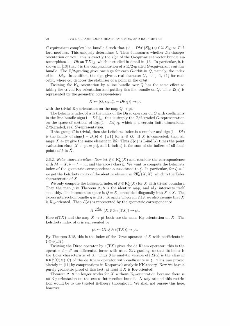
22 IVO DELL’AMBROGIO, HEATH EMERSON, AND RALF MEYER
G-equivariant complex line bundle ℓ such that (id −Db)∗(S|Q) ⊗ ℓ ∼= S|Q as Clif-ford modules. This uniquely determines ℓ. Thus ℓ measures whether Db changesorientation or not. This is exactly the sign of the G-equivariant vector bundle au-tomorphism 1−Db on TX |Q, which is studied in detail in [13]. In particular, it isshown in [13] that ℓ is the complexification of a Z/2-graded G-equivariant real linebundle. The Z/2-grading gives one sign for each G-orbit in Q, namely, the indexof id −Dbx. In addition, the sign gives a real character Gx → {−1,+1} for eachorbit, where Gx denotes the stabiliser of a point in the orbit.
Twisting the KG-orientation by a line bundle over Q has the same effect astaking the trivial KG-orientation and putting this line bundle on Q. Thus L(α) isrepresented by the geometric correspondence
X ← (Q, sign(1−Db|Q))→ pt
with the trivial KG-orientation on the map Q→ pt.The Lefschetz index of α is the index of the Dirac operator on Q with coefficients
in the line bundle sign(1 −Db)|Q; this is simply the Z/2-graded G-representationon the space of sections of sign(1 − Db)|Q, which is a certain finite-dimensionalZ/2-graded, real G-representation.
If the group G is trivial, then the Lefschetz index is a number and sign(1−Db)is the family of sign(1 − Dxb) ∈ {±1} for x ∈ Q. If X is connected, then allmaps X ← pt give the same element in kk. Thus L(α) is L-ind(α) times the pointevaluation class [X ← pt = pt], and L-ind(α) is the sum of the indices of all fixed
points of b in X.
2.6.2. Euler characteristics. Now let ξ ∈ K∗G(X) and consider the correspondence
withM = X , b = f = id, and the above class ξ. We want to compute the Lefschetzindex of the geometric correspondence α associated to ξ. In particular, for ξ = 1
we get the Lefschetz index of the identity element in kkG
0 (X,X), which is the Eulercharacteristic of X .
We only compute the Lefschetz index of ξ ∈ K∗G(X) for X with trivial boundary.
Then the map ρ in Theorem 2.18 is the identity map, and idX intersects itselfsmoothly. The intersection space is Q = X , embedded diagonally into X×X . Theexcess intersection bundle η is TX . To apply Theorem 2.18, we also assume that Xis KG-oriented. Then L(α) is represented by the geometric correspondence
XidX←−− (X, ξ ⊗ e(TX))→ pt.
Here e(TX) and the map X → pt both use the same KG-orientation on X . TheLefschetz index of α is represented by
pt← (X, ξ ⊗ e(TX))→ pt.
By Theorem 2.18, this is the index of the Dirac operator of X with coefficients inξ ⊗ e(TX).
Twisting the Dirac operator by e(TX) gives the de Rham operator: this is theoperator d + d∗ on differential forms with usual Z/2-grading, so that its index isthe Euler characteristic of X . Thus (the analytic version of) L(α) is the class in
KKG0 (C(X),C) of the de Rham operator with coefficients in ξ. This was provedalready in [11] by computations in Kasparov’s analytic KK-theory. Now we have apurely geometric proof of this fact, at least if X is KG-oriented.
Theorem 2.18 no longer works for X without KG-orientation because there isno KG-orientation on the excess intersection bundle. A way around this restric-tion would be to use twisted K-theory throughout. We shall not pursue this here,however.

EQUIVARIANT LEFSCHETZ FIXED-POINT FORMULA 23
We can now clarify the relationship between the Euler class e(TX) ∈ Kdim(X)G (X)
and the higher Euler characteristic EulX ∈ KKG0 (C(X),C) introduced alreadyin [11]. Since we assume X KG-oriented and without boundary, there is a duality
isomorphism Kdim(X)G (X) ∼= KG0 (X) = KKG0 (C(X),C). This duality isomorphism
maps e(TX) to EulX .
2.6.3. Self-maps without transversality. Let X be a compact G-manifold and letb : X → X be a smooth G-map. We want to compute the Lefschetz map on thegeometric correspondence
Xb←− X
idX−−→ X
with KG-theory class 1 on X .If b is transverse to the identity map, then this is done already in Section 2.6.1.
The case b = idX is done already in Section 2.6.2. Now we assume that b and idXintersect smoothly. We also assume that b has no fixed points on the boundary;then we may choose the collar neighbourhood of ∂X to contain no fixed points of b,so that ρ(x) = x in a neighbourhood of the fixed point subset of b. Furthermore,all fixed points of ρb are already fixed points of b.
That b and idX intersect smoothly and away from ∂X means that
Q := {x ∈ X | b(x) = x} = {x ∈ X | ρb(x) = x}
is a smooth submanifold of X and that there is an exact sequence of G-vectorbundles over Q:
0→ TQ→ TX |Q1−D(ρb)−−−−−→ TX |Q → η → 0,
where η is the excess intersection bundle.
Remark 2.20. The maps b and idX always intersect smoothly if b : X → X isisometric with respect to a Riemannian metric on X ; the reason is that if Db fixesa vector (x, ξ) at a fixed point of b, then b fixes the entire geodesic through x indirection ξ.
The vector bundles TQ and η are the kernel and cokernel of the vector bundleendomorphism 1 −D(ρb) on TX |Q. Since both are vector bundles, 1−D(ρb) haslocally constant rank. We may split
TX |Q ∼= ker(id−D(ρb))⊕ im(id−D(ρb)) = TQ⊕ im(id−D(ρb)),
TX |Q ∼= coker(id−D(ρb))⊕ coim(id−D(ρb)) = η ⊕ coim(id−D(ρb)).
Since im(ϕ) ∼= coim(ϕ) for any vector bundle homomorphism, it follows that ηand TQ are stably isomorphic as G-vector bundles. Thus KG-orientations on oneof them translate to KG-orientations on the other.
Remark 2.21. Given two stably isomorphic vector bundles, there is always a vectorbundle endomorphism with these two as kernel and cokernel. Hence we cannotexpect η and TQ to be isomorphic.
Corollary 2.22. Let X be a compact G-manifold. Let b : X → X be a smooth
G-map without fixed points on ∂X, such that b and idX intersect smoothly. Let the
fixed point submanifold Q of b be KG-oriented, and equip the excess intersection
bundle with the induced KG-orientation. Then the Lefschetz index of the geometric
correspondence
Xb←− X
idX−−→ X
with KG-theory class 1 on X is the index of the Dirac operator on Q twisted by e(η).

24 IVO DELL’AMBROGIO, HEATH EMERSON, AND RALF MEYER
The Lefschetz map sends the correspondence above to
Xbj←− Q→ pt
with K-theory class e(η) on Q.
2.6.4. Trace computation for standard correspondences. By Corollary 2.8, any ele-
ment of kkG
∗ (X,X) is represented by a correspondence of the form
Xι◦π◦pr
1←−−−−− NX ×Xpr
2−−→ X
for a unique ξ ∈ K∗G(NX×X). We may view this as a standard form for an element
in kkG
∗ (X,X).
The map (ρ◦ι◦π◦pr1, pr2) = (ρ◦π)× id : NX×X → X×X is a submersion andhence transverse to the diagonal. Thus Theorem 2.18 applies. The spaceQρb,f is the
graph of ρπ : NX → X . Thus the Lefschetz map gives the geometric correspondence
X ← NX → pt, ξ|NX ∈ K∗G(NX),
where we embed NX → NX ×X via (id, ρπ) and use the canonical KG-orientation
on NX . The Lefschetz index in kkG
∗ (pt, pt) ∼= K∗G(pt) is computed analytically as
the G-equivariant index of the Dirac operator on NX twisted by ξ|NX .
2.6.5. Trace computation for another standard form. Assume now that X has noboundary and is KG-oriented. As we remarked at the end of Section 2.4, any
element of kkG
∗ (X,X) is represented by a correspondence
Xpr
1←−− X ×Xpr
2−−→ X, ξ ∈ K∗G(X ×X).
The same computation as in Section 2.6.4 shows that the Lefschetz map sends thisto
X = X → pt, ξ|X ∈ K∗G(X),
where ξ|X is for the diagonal embedding X → X × X . Analytically, this is theKG-homology class of the Dirac operator on X with coefficients ξ|X .
2.6.6. Homogeneous correspondences. We call a self-correspondence Xb←−M
f−→ X
homogeneous if X and M are homogeneous G-spaces. That is, X := G/H andM := G/L for closed subgroups H,L ⊆ G. Then there are elements tb, tf ∈ G with
b(gL) := gtbH , f(gL) := gtfH ; we need L ⊆ tbHt−1b ∩ tfHt
−1f for this to be well-
defined. Since G/L ∼= G/t−1f Ltf by gL 7→ gLtf , any homogeneous correspondence
is isomorphic to one with tf = 1, so that L ⊆ H . We assume this from now on andabbreviate t = tb.
Since M and X are compact, the relevant K-theory group RK∗G,X(M) for a
homogeneous correspondence is just K∗G(M). The induction isomorphism gives
RK∗G,X(M) = K∗
G(G/L)∼= K∗
L(pt).
A KG-orientation for f : G/L → G/H is equivalent to a KH -orientation for theprojection map H/L → pt because f is obtained from this H-map by induction.
Thus we must assume an KH -orientation on H/L. Equivalently, the representationof L on T1L(H/L) factors through Spinc. This tangent space is the quotient h/l,where h and l denote the Lie algebras of H and L, respectively.
Let L′ := H ∩ tHt−1. Then L ⊆ L′ and both maps f, b : G/L → G/H factorthrough the quotient map p : G/L→ G/L′. The geometric correspondence
G/Hb←− G/L
f−→ G/H, ξ ∈ K∗
G(G/L)
is equivalent to the geometric correspondence
G/Hb′
←− G/L′ f ′
−→ G/H, ξ′ ∈ K∗G(G/L
′)

EQUIVARIANT LEFSCHETZ FIXED-POINT FORMULA 25
with ξ′ := p!(ξ) and b′(gL′) = gtH and f ′(gL′) = gH . (To construct the equiv-alence, we first need a normally non-singular map lifting p; then we apply vectorbundle modifications on the domain and target of p to replace p by an open embed-ding; finally, for an open embedding we may construct a bordism as in [15, Example2.14].)
Thus we may further normalise a homogeneous geometric self-correspondence toone with L = H ∩ tHt−1.
Now we compute the Lefschetz map for a such a normalised homogeneous self-correspondence.
First let t /∈ H . Then the image of the map (f, b) : G/L → G/H × G/H doesnot intersect the diagonal. Hence (f, b) is transverse to the diagonal and the coin-cidence space Qb,f is empty. Thus the Lefschetz map vanishes on a homogeneouscorrespondence with t /∈ H by Theorem 2.18.
Now let t ∈ H . Then b = f : G/L→ G/H is the canonical projection map. Ournormalisation condition yields L = H and b = f = id in this case; that is, our
geometric correspondence is the class in kkG
∗ (G/H,G/H) of some ξ ∈ K∗G(G/H).
Thus we have a special case of the Euler characteristic computation in Section 2.6.2.The Lefschetz map gives the class of the geometric correspondence
G/Hid←−
=(G/H, e(TG/H)⊗ ξ)→ pt,
provided G/H is KG-oriented. The Lefschetz index is the index of the de Rhamoperator with coefficients in ξ.
When we identify K∗G(G/H) ∼= K∗
H(pt), the Lefschetz index becomes a map
K∗H(pt)→ K∗
G(pt).
In complex K-theory, this is a map R(H)→ R(G). Graeme Segal studied this mapin [28, Section 2], where it was denoted by i!.
For instance, assume G to be connected and let H = L be its maximal torus. Lett ∈W := NGH/H , the Weyl group ofG. Assume that we are working with complexK-theory, so that K∗
G(G/H) ∼= K∗H(pt) ∼= R(H). The Weyl group W acts on G/H
by right translations; these are G-equivariant maps. Taking the correspondences
Xw−1
←−−− X = X , this gives a representation W → kkG
0 (G/H,G/H). We also map
R(H) ∼= K0G(G/H) → kk
G
0 (G/H,G/H) using the correspondences X = (X, ξ) =X . These representations of W and R(H) are a covariant pair of representationswith respect to the canonical action of W on R(H) induced by the automorphismsh 7→ whw−1 of H for w ∈W . Hence we map
R(H)⋊W → kkG
0 (G/H,G/H).
The Lefschetz index R(H) ⋊ W → R(G) maps a · t 7→ 0 for t ∈ W \ {1} anda · 1 7→ indG Λa, where Λa means the de Rham operator on G/H twisted by a.
2.7. Fixed points submanifolds for torus actions. As another application ofour excess intersection formula, we reprove a result that is used in a recent articleby Block and Higson [5] to reformulate the Weyl Character Formula in KK-theory.
Block and Higson also develop a more geometric framework for equivariantKK-theory for a compact group. For two locally compact G-spaces X and Y ,they identify KKG∗ (X,Y ) with the group of continuous natural transformationsΦZ : K∗
G(X × Z)→ K∗G(Y ×Z) for all compact G-spaces Z; here continuity means
that each ΦZ is a K∗G(Z)-module homomorphism. The Kasparov product then be-
comes the composition of natural transformations. This reduces Kasparov’s equi-variant KK-theory to equivariant K-theory.

26 IVO DELL’AMBROGIO, HEATH EMERSON, AND RALF MEYER
The theory kkGdoes more: it contains the knowledge that all such natural trans-
formations come from geometric correspondences, when geometric correspondencesgive the same natural transformation, and how to compose geometric correspon-dences. Thus we get a more concrete KK-theory.
Theorem 2.23. Let T be a compact torus and let X be a smooth, KT -oriented
T -manifold with boundary. Let e(TX) ∈ K0T (X) be the Euler class of X for the
chosen KT -orientation. Let F ⊆ X be the fixed-point subset of the T -action on Xand let j : F → X be the inclusion map. Then F is again a smooth K-oriented mani-
fold with boundary, with trivial T -action, so that the inclusion map j is KT -oriented.
Let e(TF ) ∈ K0(F ) ⊆ K0T (F ) be the Euler class of F . The two geometric corre-
spondences
XidX←−− (X, e(TX))
idX−−→ X,
Xj←− (F, e(TF ))
j−→ X
represent the same element in kkT
0 (X,X).
This is a generalisation of [5, Lemma 3.1]. We allow Spinc-manifolds instead ofcomplex manifolds. For a Spinc-structure coming from a complex structure, theEuler class is [Λ∗T∗X ] ∈ K0
T (X), which appears in [5]. The following proof is a
translation of the proof in [5] into the category kkG.
Proof. The first geometric correspondence above, involving the Euler class of X , isrepresented by the composition of geometric correspondences
XidX←−−=
Xζ−→ TX
ζ←− X
idX−−→=
X
by Example 2.13; here ζ denotes the zero section, which is KT -oriented using thegiven KT -orientation on the T -vector bundle TX .
Choose a generic element ξ in the Lie algebra of T , that is, the one-parametergroup exp(sξ), s ∈ R, is dense in T . Let αt : X → X denote the action of t ∈ Ton X . The action of T maps ξ to a vector field αξ : X → TX . There is a homotopyof geometric correspondences
XidX←−−=
Xαsξ−−→ TX
ζ←− X
idX−−→=
X
for s ∈ [0, 1]. For t = 0 we get the composition above, involving e(TX). We claimthat for s = 1, the two correspondences intersect smoothly and that the intersectionproduct is the second geometric correspondence in the theorem, involving F andits Euler class.
First we show that the fixed-point submanifold F is a closed submanifold. EquipXwith a T -invariant Riemannian metric. Let x ∈ F , that is, αt(x) = x for all t ∈ T .Split TxX into
V = {v ∈ TxX | Dαt(x, v) = (x, v) for all t ∈ T }
and its orthogonal complement V ⊥. Since the metric is T -invariant, αt(exp(x, v)) =exp(Dαt(x, v)) for all v ∈ TxX . Since the exponential mapping restricts to adiffeomorphism between a neighbourhood of 0 in TxX and a neighbourhood of xin X , we have exp(x, v) ∈ F if v ∈ V , and the converse holds for v in a suitableneighbourhood of 0. Thus we get a closed submanifold chart for F near x withTxF = V . Hence F is a closed submanifold with
TF = {(x, v) ∈ TX | Dαt(x, v) = (x, v) for all t ∈ T }.
Since ξ is generic, αξ(x) = 0 in TxX if and only if x ∈ F . Thus F is the coinci-dence space of the pair of maps ζ, αξ : X → TX . Let x ∈ F and let v1, v2 ∈ TxX

EQUIVARIANT LEFSCHETZ FIXED-POINT FORMULA 27
satisfy Dζ(x, v1) = Dαξ(x, v2). Then v1 = v2 by taking the horizontal com-ponents; and the vertical component of Dαξ(x, v2) vanishes, which means thatDαexp(sξ)(x, v2) = (x, v2) for all s ∈ R. Hence v2 ∈ TxF . This proves that ζ and αξintersect smoothly. The excess intersection bundle is the cokernel of Dαexp(sξ)− id;since the action of T is by isometries, Dαexp(sξ)− id is normal in each fibre, so thatits image and kernel are orthogonal complements. Hence the cokernel is canonicallyisomorphic to the kernel of Dαexp(sξ) − id. Thus the excess intersection bundle iscanonically isomorphic to TF .
Hence Theorem 2.17 gives the geometric correspondence Xj←− (F, e(TF ))
j−→ X
as the composition, as desired. �
3. The homological Lefschetz index of a Kasparov morphism
The example in Section 2.6.1 shows in what sense the geometric Lefschetz indexcomputations in Section 2 generalise the local fixed-point formula for the Lefschetzindex of a self-map. Now we turn to generalisations of the global homologicalformula for the Lefschetz index.
The classical Lefschetz fixed-point formula for a self-map f : X → X contains the(super)trace of the map on the cohomology of X with rational coefficients inducedby f . We take rational coefficients in order to get vector spaces over a field, wherethere is a good notion of trace for endomorphisms. By the Chern character, we mayas well take K∗(X)⊗Q instead of rational cohomology. It is checked in [9] that theLefschetz index of f ∈ KK0(A,A) for a dualisable C∗-algebra A in the bootstrapclass is equal to the supertrace of the map on K∗(A)⊗Q induced by f .
We are going to generalise this result to the equivariant situation for a com-pact Lie group G. We assume that we are working with complex C∗-algebras, so
that kkG
∗ (pt, pt) = KKG∗ (C,C) vanishes in odd degrees and is the representationring R(G) in even degrees. Our methods do not apply to the torsion invariants
in KKGd (R,R) for d 6= 0 in the real case because we (implicitly) tensor everythingwith Q to simplify the Lefschetz index.
Furthermore, we work in KKG instead of kkG
in this section because the cate-
gory KKG is triangulated, unlike kkG. We explain in Remark 3.11 why kk
Gis not
triangulated; the triangulated structure on KKG is introduced in [21].Let S ⊆ R(G) be the set of all elements that are not zero divisors. This is a
saturated, multiplicatively closed subset; even more, it is the largest multiplicativelyclosed subset for which the canonical map R(G)→ S−1 R(G) to the ring of fractionsis injective (see [1, Exercise 9 on p. 44]). The localisation S−1 R(G) is also calledthe total ring of fractions of R(G).
Since KKG is symmetric monoidal with unit 1 = C and R(G) = KKG0 (C,C),
the category KKG is R(G)-linear. Hence we may localise it at S as in [17]. The
resulting category T := S−1KKG has the same objects as KKG and arrows
T∗(A,B) := S−1KKG∗ (A,B) = S−1 R(G) ⊗R(G) KKG∗ (A,B).
The category T is S−1 R(G)-linear. There is an obvious functor ♮ : KKG → T .If A is a separable G-C∗-algebra, then
T∗(C, A) = S−1KKG∗ (C, A) ∼= S−1 R(G)⊗R(G) KG∗ (A),
where we use the usual R(G)-module structure on KG∗ (A) ∼= KKG∗ (C, A).There is a unique symmetric monoidal structure on T for which ♮ is a strict
symmetric monoidal functor: simply extend the exterior tensor product on KKG
S−1 R(G)-linearly. Hence if A is dualisable in KKG, then its image in T is dualisable

28 IVO DELL’AMBROGIO, HEATH EMERSON, AND RALF MEYER
as well, and
♮(tr f) = tr(♮f) for all f ∈ KKG∗ (A,A).
The crucial point for us is that ♮ tr(f) = tr(♮f) uniquely determines tr f becausethe map
R(G) ∼= KKG0 (1,1)♮−→ T0(1,1) ∼= S−1 R(G)
is injective. Thus it suffices to compute Lefschetz indices in T . This may be easierbecause T has more isomorphisms and thus fewer isomorphism classes of objects.Furthermore, the endomorphism ring of the unit T∗(1,1) = S−1 R(G) has a rathersimple structure:
Lemma 3.1. The ring S−1 R(G) is a product of finitely many fields.
Proof. Let G/AdG be the space of conjugacy classes in G and let C(G/AdG)be the algebra of continuous functions on G/AdG. Taking characters provides aring homomorphism χ : R(G) → C(G/AdG), which is well-known to be injective.Hence R(G) is torsion-free as an Abelian group and has no nilpotent elements.Since G is a compact Lie group, R(G) is a finitely generated commutative ring by[28, Corollary 3.3]. Thus R(G) is Noetherian and reduced. This implies that itstotal ring of fractions is a finite product of fields (see [18, Exercise 6.5]). �
The fields in this product decomposition correspond bijectively to minimal primeideals in R(G). By [28, Proposition 3.7.iii], these correspond bijectively to cyclicsubgroups of G/G0, where G0 denotes the connected component of the identityelement. In particular, S−1 R(G) is a field if and only if G is connected.
Example 3.2. Let G be a connected compact Lie group. Let T be a maximaltorus in G and let W be the Weyl group, W := NG(T )/T . Highest weight theoryprovides an isomorphism R(G) ∼= R(T )W . Here R(T ) is a ring of integral Laurentpolynomials in r variables, where r is the rank of T . Since elements of N≥1 arenot zero divisors in R(G), the total ring of fractions of R(G) is equal to the totalring of fractions of R(G)⊗Q. The latter is the Q-algebra of W -invariant elementsin Q[x1, . . . , xr , (x1 · · ·xr)−1]. This is the algebra of polynomial functions on thealgebraic Q-variety (Q×)r, and the W -invariants give the algebra of polynomialson the quotient variety (Q×)r/W . This variety is connected, so that the total ringof fractions S−1 R(G) in this case is the field of rational functions on the algebraicQ-variety (Q×)r/W .
Now we can define an equivariant analogue of the trace of the map on K∗(A)⊗Q
induced by f ∈ KK0(A,A):
Definition 3.3. Let S−1 R(G) =∏ni=1 Fi with fields Fi. A module over S−1 R(G)
is a product∏ni=1 Vi, where each Vi is an Fi-vector space. In particular, if A is
a G-C∗-algebra, then T∗(C, A) = S−1KG∗ (A) =∏ni=1 K
G∗,i(A) for certain Z/2-graded
Fi-vector spaces KG∗,i(A). An endomorphism f ∈ T0(A,A) induces grading-preserving
endomorphisms KG∗,i(f) : KG∗,i(A)→ KG∗,i(A).
If the vector spaces KG∗,i(A) are all finite-dimensional, then the (super)trace of
KG∗,i(f) is defined to be trKG0,i(f)− trKG1,i(f) ∈ Fi, and
trS−1KG∗ (f) := (trKG∗,i(f))ni=1 ∈
n∏
i=1
Fi = S−1 R(G).
We will see below that dualisability for objects in appropriate bootstrap classesalready implies that KG∗ (A) is a finitely generated R(G)-module, and then each
KG∗,i(A) must be a finite-dimensional Fi-vector space.
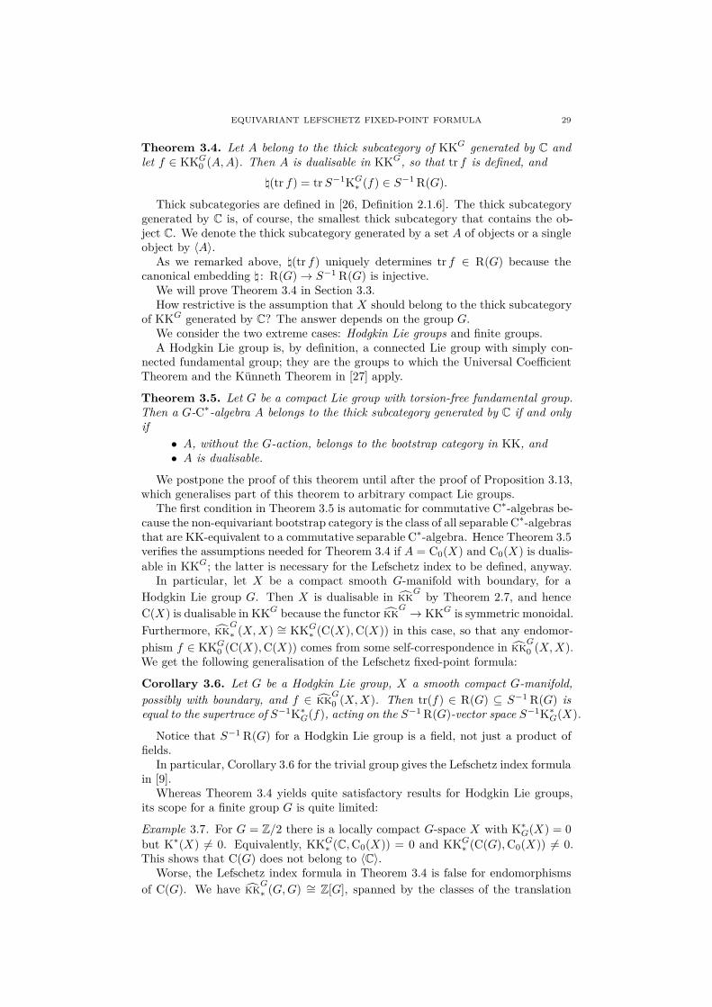
EQUIVARIANT LEFSCHETZ FIXED-POINT FORMULA 29
Theorem 3.4. Let A belong to the thick subcategory of KKG generated by C and
let f ∈ KKG0 (A,A). Then A is dualisable in KKG, so that tr f is defined, and
♮(tr f) = trS−1KG∗ (f) ∈ S−1 R(G).
Thick subcategories are defined in [26, Definition 2.1.6]. The thick subcategorygenerated by C is, of course, the smallest thick subcategory that contains the ob-ject C. We denote the thick subcategory generated by a set A of objects or a singleobject by 〈A〉.
As we remarked above, ♮(tr f) uniquely determines tr f ∈ R(G) because thecanonical embedding ♮ : R(G)→ S−1 R(G) is injective.
We will prove Theorem 3.4 in Section 3.3.How restrictive is the assumption that X should belong to the thick subcategory
of KKG generated by C? The answer depends on the group G.We consider the two extreme cases: Hodgkin Lie groups and finite groups.A Hodgkin Lie group is, by definition, a connected Lie group with simply con-
nected fundamental group; they are the groups to which the Universal CoefficientTheorem and the Künneth Theorem in [27] apply.
Theorem 3.5. Let G be a compact Lie group with torsion-free fundamental group.
Then a G-C∗-algebra A belongs to the thick subcategory generated by C if and only
if
• A, without the G-action, belongs to the bootstrap category in KK, and
• A is dualisable.
We postpone the proof of this theorem until after the proof of Proposition 3.13,which generalises part of this theorem to arbitrary compact Lie groups.
The first condition in Theorem 3.5 is automatic for commutative C∗-algebras be-cause the non-equivariant bootstrap category is the class of all separable C∗-algebrasthat are KK-equivalent to a commutative separable C∗-algebra. Hence Theorem 3.5verifies the assumptions needed for Theorem 3.4 if A = C0(X) and C0(X) is dualis-
able in KKG; the latter is necessary for the Lefschetz index to be defined, anyway.In particular, let X be a compact smooth G-manifold with boundary, for a
Hodgkin Lie group G. Then X is dualisable in kkG
by Theorem 2.7, and hence
C(X) is dualisable in KKG because the functor kkG→ KKG is symmetric monoidal.
Furthermore, kkG
∗ (X,X) ∼= KKG∗ (C(X),C(X)) in this case, so that any endomor-
phism f ∈ KKG0 (C(X),C(X)) comes from some self-correspondence in kkG
0 (X,X).We get the following generalisation of the Lefschetz fixed-point formula:
Corollary 3.6. Let G be a Hodgkin Lie group, X a smooth compact G-manifold,
possibly with boundary, and f ∈ kkG
0 (X,X). Then tr(f) ∈ R(G) ⊆ S−1 R(G) is
equal to the supertrace of S−1K∗G(f), acting on the S−1 R(G)-vector space S−1K∗
G(X).
Notice that S−1 R(G) for a Hodgkin Lie group is a field, not just a product offields.
In particular, Corollary 3.6 for the trivial group gives the Lefschetz index formulain [9].
Whereas Theorem 3.4 yields quite satisfactory results for Hodgkin Lie groups,its scope for a finite group G is quite limited:
Example 3.7. For G = Z/2 there is a locally compact G-space X with K∗G(X) = 0
but K∗(X) 6= 0. Equivalently, KKG∗ (C,C0(X)) = 0 and KKG∗ (C(G),C0(X)) 6= 0.This shows that C(G) does not belong to 〈C〉.
Worse, the Lefschetz index formula in Theorem 3.4 is false for endomorphisms
of C(G). We have kkG
∗ (G,G)∼= Z[G], spanned by the classes of the translation

30 IVO DELL’AMBROGIO, HEATH EMERSON, AND RALF MEYER
maps G→ G, x 7→ x · g for g ∈ G, and these are homogeneous correspondences asin Section 2.6.6.
Translation by g = 1 is the identity map, and its Lefschetz index is the classof the regular representation of G in R(G). For g 6= 1, the Lefschetz index iszero because the fixed point subset is empty. However, K∗
G(G) = K∗(pt) = Z[0]and all translation maps induce the identity map on K∗
G(G). Thus the inducedmap on K∗
G(G) is not enough information to compute the Lefschetz index of an
endomorphism of G in kkG.
3.1. The equivariant bootstrap category. A reasonable Lefschetz index for-mula should apply at least to KKG-endomorphisms of C(X) for all smooth compactG-manifolds and thus, in particular, for finite G-sets X . Example 3.7 shows thatTheorem 3.4 fails on such a larger category. This leads us to improve the Lefschetzindex formula. First we discuss the class of G-C∗-algebras where we expect it tohold.
We are going to describe an equivariant analogue of the bootstrap class in KKG.Our class is larger than the class of C∗-algebras that are KKG-equivalent to acommutative C∗-algebra. The latter subcategory is too small because it is notthick. The thick (or localising) subcategory of KKG generated by commutativeC∗-algebras is a better choice, but such a definition is not very intrinsic. We willchoose an even larger subcategory of KKG because it is not more difficult to treatand has a nicer characterisation.
The category KKG only has countable coproducts because we need C∗-algebrasto be separable. Hence the standard notions of compact objects and localisingsubcategories have to be modified so that they only involve countable coproducts.As in [7, Definition 2.1], we speak of compactℵ1
objects, localisingℵ1subcategories,
and compactlyℵ1generated subcategories.
Definition 3.8. Call a G-C∗-algebra A elementary if it is of the form IndGH MnC =C(G,MnC)
H for some closed subgroup H ⊆ G and some action of H on MnC byautomorphisms; the superscript H means the fixed points for the diagonal actionof H .
Definition 3.9. Let BG ⊆ KKG be the localisingℵ1subcategory generated by all
elementary G-C∗-algebras. We call BG the G-equivariant bootstrap category.
An action of H on MnC comes from a projective representation of H on Cn.Such a projective representation is a representation of an extension of H by thecircle group. The extension is classified by a cohomology class in H2(H,U(1)). Twoactions on MnC are H-equivariantly Morita equivalent if and only if they belongto the same class in H2(H,U(1)). The G-C∗-algebras IndGH MnC for actions of H
on MnC with different cohomology classes need not be KKG-equivalent.
Theorem 3.10. A G-C∗-algebra belongs to the localisingℵ1subcategory generated
by the elementary G-C∗-algebras if and only if it is KKG-equivalent to a G-action
on a type I C∗-algebra.
Proof. It is already shown in [27, Theorem 2.8] that allG-actions on type I C∗-algebrasbelong to the localisingℵ1
subcategory generated by the elementary G-C∗-algebras.
By definition, localisingℵ1subcategories are closed under KKG-equivalence. Ele-
mentary G-C∗-algebras are type I C∗-algebras, even continuous trace C∗-algebras.To finish the proof we must show that the G-C∗-algebras that are KKG-equivalentto type I G-C∗-algebras form a localisingℵ1
subcategory of KKG.
Let T1 ⊆ KKG be the full subcategory of type I, separable G-C∗-algebras. IfA ∈ T1, then C0(R, A) ∈ T1, so that T1 is closed under suspension and desuspension.

EQUIVARIANT LEFSCHETZ FIXED-POINT FORMULA 31
Let A,B ∈ T1 and f ∈ KKG0 (A,B). We have KKG0 (A,B) ∼= KKG1 (A,C0(R, B)),and cycles for the latter group correspond to (equivariantly) semisplit extensionsof G-C∗-algebras
C0(R, B)⊗K D ։ A
with K := K(L2(G × N)). Since B and A are type I, so are C0(R, B) ⊗ K and Dbecause the property of being type I is inherited by extensions. The semisplitextension above provides an exact triangle isomorphic to
B[−1]→ D → Af−→ B.
Thus there is an exact triangle containing f with all three entries in T1. Furthermore,countable direct sums of type I C∗-algebras are again type I. This implies thatthe G-C∗-algebras KKG-equivalent to one in T1 form a localisingℵ1
subcategory
of KKG. �
Remark 3.11. In the non-equivariant case, any C∗-algebra in the bootstrap classis KK-equivalent to a commutative one. This criterion fails already for G = U(1),as shown by a counterexample in [10]. Since the bootstrap class is the smallestlocalising subcategory containing C, it follows that the commutative C∗-algebras
do not form a localising subcatgory. Thus kkG
is not triangulated: it lacks conesfor some maps.
In this case, the equivariant bootstrap class is already generated by C and con-tains all U(1)-actions on C∗-algebras in the non-equivariant bootstrap category. Itis shown in [10] that the U(1)-equivariant K-theory of a suitable Cuntz–Krieger al-gebra with its natural gauge action cannot arise from any U(1)-action on a locallycompact space.
Corollary 3.12. The restriction and induction functors KKG → KKH and KKH →KKG for a closed subgroup H in a compact Lie group G restrict to functors between
the bootstrap classes in KKG and KKH .
Proof. Restriction does not change the underlying C∗-algebra and thus preservesthe property of being type I. Induction maps elementary H-C∗-algebras to elemen-tary G-C∗-algebras, is triangulated, and commutes with direct sums. Hence itmaps BH to BG. �
Proposition 3.13. An object of BG is compactℵ1if and only if it is dualisable, if
and only if it belongs to the thick subcategory of BG (or of KKG) generated by the
elementary G-C∗-algebras.
Proof. The tensor unit C is compactℵ1because KKG∗ (C, A) ∼= KG∗ (A)
∼= K∗(G⋉A)is countable for all G-C∗-algebras A, and the functors A 7→ G ⋉ A and K∗ arewell-known to commute with coproducts. Furthermore, the tensor product in KKG
commutes with coproducts in both variables.Using this, we show that dualisable objects of BG are compactℵ1
. If A is dualis-
able with dual A∗, then KKG(A,B) ∼= KKG(C, A∗ ⊗B), and since C is compactℵ1
and ⊗ commutes with countable direct sums, it follows that A is compactℵ1.
It follows from [8, Corollary 2.2] that elementary G-C∗-algebras are dualisableand hence compactℵ1
. A compact group has only at most countably many com-pact subgroups by Lemma 3.14 below; and any of them has at most finitely manyprojective representations. Hence the set of elementary G-C∗-algebras is at mostcountable. Therefore, BG is compactlyℵ1
generated in the sense of [7, Definition2.1]. By [7, Corollary 2.4] an object of BG is compactℵ1
if and only if it belongs tothe thick subcategory generated by the elementary G-C∗-algebras.
32 IVO DELL’AMBROGIO, HEATH EMERSON, AND RALF MEYER
The Brown Representability Theorem [7, Corollary 2.2] shows that for everycompactℵ1
object A of BG there is a functor Hom(A, ␣) from BG to BG such that
KKG(A⊗B,D) ∼= KKG(B,Hom(A,D))
for all B,D in BG. Using exactness properties of the internal Hom functor inthe first variable, we then show that the class of dualisable objects in BG is thick(see [7, Section 2.3]). Thus all objects of the thick subcategory generated by theelementary G-C∗-algebras are dualisable. �
The following lemma is well-known, see for example [25].
Lemma 3.14. A compact Lie group has at most countably many conjugacy classes
of closed subgroups.
Proof. Let H be a closed subgroup of a compact Lie group G. By the MostowEmbedding Theorem, G/H embeds into a linear representation of G, that is, H isa stabiliser of a point in some linear representation of G. Up to isomorphism, thereare only countably many linear representations of G. Each linear representationhas finite orbit type, that is, it admits only finitely many different conjugacy classesof stabilisers. Hence there are altogether at most countably many conjugacy classesof closed subgroups in G. �
Proof of Theorem 3.5. Let G be a Hodgkin Lie group. The main result of [23] says
that A belongs to the localising subcategory of KKG generated by C if and only ifA⋊G belongs to the non-equivariant bootstrap category (this is special for HodgkinLie groups). Since this covers all elementary G-C∗-algebras, we conclude that thelocalising subcategory generated by C contains BG and is, therefore, equal to BG.
The same argument as in the proof of Proposition 3.13 shows that the followingare equivalent for an object A of BG:
• A is dualisable;• A is compactℵ1
;• A belongs to the thick subcategory generated by C.
This finishes the proof of Theorem 3.5. �
So far we always used the bootstrap class, which is the domain where a UniversalCoefficient Theorem holds. The next proposition is a side remark showing that wemay also use the domain where a Künneth formula holds.
Definition 3.15. An object A ∈ KKG satisfies the Künneth formula if KG∗ (A ⊗B) = 0 for all B that satisfy KG∗ (C ⊗B) = 0 for all elementary G-C∗-algebras C.
By results of [20,24], the assumption in Definition 3.15 is necessary and sufficient
for a certain natural spectral sequence that computes KG∗ (A⊗B) from KKG∗ (C,A)
and KKG∗ (C,B) for elementary C to converge for all B; we have no need to describethis spectral sequence.
Proposition 3.16. Let A ∈ KKG be dualisable with dual A∗. If A or A∗ satisfies
a Künneth formula, then both A and A∗ belong to BG, and vice versa.
Proof. Since BG is generated by the elementary G-C∗-algebras, KKG∗ (C,B) = 0
for all elementary G-C∗-algebras C if and only if KKG∗ (C,B) = 0 for all C ∈ BG.Any elementary G-C∗-algebra C is dualisable with a dual in BG. Hence KG∗ (C ⊗B) ∼= KKG∗ (C∗, B) = 0 for elementary C if KKG∗ (C′, B) = 0 for all elementary
G-C∗-algebras C′; conversely KKG∗ (C,B) ∼= KG∗ (C∗ ⊗ B) = 0 for elementary C if
KG∗ (C′ ⊗ B) = 0 for all elementary G-C∗-algebras C′. Let us denote the class ofG-C∗-algebras with these equivalent properties BG,⊥.

EQUIVARIANT LEFSCHETZ FIXED-POINT FORMULA 33
It follows from [20, Theorem 3.16] that (BG,BG,⊥) is a complementary pair of
localising subcategories. In particular, if KKG∗ (A,B) = 0 for all B ∈ BG,⊥, thenA ∈ BG.
Now assume, say, that A satisfies a Künneth formula. Then KKG∗ (A∗, B) ∼=KG∗ (A ⊗ B) = 0 for all B ∈ BG,⊥. Thus A∗ ∈ BG. Then KG∗ (A
∗ ⊗ B) = 0 for all
B ∈ BG,⊥ because the class of C with KG∗ (C ⊗B) = 0 is localising and contains allelementary C if B ∈ BG,⊥. As above, this implies (A∗)∗ = A ∈ BG. �
The proof of Theorem 3.5 above used that, for a Hodgkin Lie group, BG is alreadygenerated by C. For more general groups, we also expect that fewer generatorssuffice to generate BG. But we only need and only prove a result about topologicallycyclic groups here.
A locally compact group G is called topologically cyclic if there is an elementg ∈ G that generates a dense subgroup of G. A topologically cyclic group isnecessarily Abelian. We are interested in topologically cyclic, compact Lie groupshere. A compact Lie group is topologically cyclic if and only if it is isomorphic toTr × F for some r ≥ 0 and some finite cyclic group F (possibly the trivial group),where T = R/Z ∼= U(1). Here we use that any extension Tr E ։ F for a finitecyclic group F splits. This also implies that any projective representation of a finitecyclic groups is a representation.
Theorem 3.17. Let G be a topologically cyclic, compact Lie group. Then the
bootstrap class BG ⊆ KKG is already generated by the finitely many G-C∗-algebras
C(G/H) for all open subgroups H ⊆ G.
Furthermore, an object of BG is compactℵ1if and only if it is dualisable if and
only if it belongs to the thick subcategory generated by C(G/H) for open subgroups
H ⊆ G.
Proof. The second statement about compactℵ1objects in BG follows from the first
one and [7, Corollary 2.4], compare the proof of Proposition 3.13. Thus it sufficesto prove that the objects C(G/H) for open subgroups already generate BG. Forthis, we use an isomorphism G ∼= Tr × F for some r ≥ 0 and some finite cyclicsubgroup F .
Let us first consider the special case r = 0, that is, G is a finite cyclic group.In this case, any subgroup of G is open and again cyclic. We observed above thatcyclic groups have no non-trivial projective representations. Thus any elementaryG-C∗-algebra is Morita equivalent to C(G/H) for some open subgroup H in G.Hence the assertion of the theorem is just the definition of BG in this case.
If F is trivial, then the assertion follows from Theorem 3.5. Now we considerthe general case where both F and Tr are non-trivial.
The Pontryagin dual G of G is isomorphic to the discrete group Zr × F . If Ais a G-C∗-algebra, then G ⋉ A carries a canonical action of G called the dualaction. Similarly, G ⋉ A for a G-C∗-algebra A carries a canonical dual action
of G. This provides functors KKG → KKG and KKG → KKG. Baaj–Skandalisduality says that they are inverse to each other up to natural equivalence (see[2, Section 6]). Since both functors are triangulated, this is an equivalence oftriangulated categories.
If A is type I, then so is G ⋉ A. Hence all objects in BG ⊆ KKG are KKG-equivalent to a G-action on a type I C∗-algebra by Theorem 3.10.
The group G is Abelian and hence satisfies a very strong form of the Baum–Connes conjecture: it has a dual Dirac morphism and γ = 1 in the sense of [22, Def-
inition 8.1]. From this it follows that any G-C∗-algebra A belongs to the localising
34 IVO DELL’AMBROGIO, HEATH EMERSON, AND RALF MEYER
subcategory of KKG that is generated by IndGHA for finite subgroups H ⊆ G (this
is shown as in the proof of [22, Theorem 9.3]).
The finite subgroups in Zr × F are exactly the subgroups of F , of course. Sincewe have induction in stages, we may assume H = F . Thus the subcategory of
type I G-C∗-algebras is already generated by IndGFA for type I F -C∗-algebras A.
Since F is a finite cyclic group, the discussion above shows that the category oftype I F -C∗-algebras A is already generated by C0(F /H) for subgroups H ⊆ F .
Thus BG is generated by the G-C∗-algebras IndGFC0(F /H) ∼= C0(G/H). The finite
subgroups H ⊆ G are exactly the orthogonal complements of (finite-index) opensubgroups H ⊆ G.
Now G ⋉ C0(G/H) is Morita equivalent to C∗(H) ∼= C0(G/H) for any open
subgroupH ⊆ G, where H ⊆ G denotes the orthogonal complement ofH in G. Thedual action on C0(G/H) comes from the translation action of G. Thus the G- and
G-C∗-algebras C0(G/H) and C0(G/H) correspond to each other via Baaj–Skandalisduality. We conclude that the G-C∗-algebras C0(G/H) for open subgroups H ⊆ Ggenerate BG. �
Let G be topologically cyclic, say, G ∼= Tr × Z/k for some r ≥ 0, k ≥ 1. Thenopen subgroups of G correspond to subgroups of Z/k and thus to divisors d of k.The representation ring of G is
(3.1) R(G) ∼= R(Tr)⊗ R(Z/k) ∼= Z[x1, . . . , xr, (x1 · · ·xr)−1]⊗ Z[t]/(tk − 1).
Lettk − 1 =
∏
d|k
Φd(t)
be the decomposition into cyclotomic polynomials. Each factor Φd generates aminimal prime ideal of R(G), and these are all minimal prime ideals of R(G). Thelocalisation at this prime ideal gives the field Q(θd)(x1, . . . , xr) of rational functionsin r variables over the cyclotomic field Q(θd), and the product of these localisationsis the total ring of fractions of R(G),
S−1 R(G) =∏
d|k
Q(θd)(x1, . . . , xr).
(Compare Lemma 3.1.)
Lemma 3.18. Let H ( G be a proper open subgroup. The canonical map
R(G)→ KKG0 (C(G/H),C(G/H))
from the exterior product in KKG factors through the restriction map R(G) →R(H). The image of C(G/H) in the localisation of KKG at the prime ideal (Φk)vanishes.
Proof. The exterior product of the identity map on C(G/H) and ξ ∈ R(G) ∼=KKG0 (C,C) is given by the geometric correspondence G/H = G/H = G/H withthe class p∗(ξ) ∈ K0
G(G/H), where p : G/H → pt is the constant map. Now identifyK0G(G/H) ∼= K0
H(pt) ∼= R(H) and p∗ with the restricton map R(G)→ R(H) to getthe first statement.
We have H ∼= Tr × Z/d embedded via (x, j) 7→ (x, jk/d) into G ∼= Tr × Z/k. IfH 6= G, then d 6= k. The restriction map R(G)→ R(H) annihilates the polynomial(tk−1)/Φk =
∏d|k,d 6=k Φd. This polynomial does not belong to the prime ideal (Φk)
and hence becomes invertible in the localisation of R(G) at (Φk). Since an invertibleendomorphism can only be zero on the zero object, C(G/H) becomes zero in the
localisation of KKG at (Φk). �

EQUIVARIANT LEFSCHETZ FIXED-POINT FORMULA 35
3.2. Localisation of the bootstrap class.
Proposition 3.19. Let G ∼= Tr × Z/k be topologically cyclic. Let BGd be the thick
subcategory of dualisable objects in the bootstrap class BG ⊆ KKG. Any object in
the localisation of BGd at the prime ideal (Φk) in R(G) is isomorphic to a finite
direct sum of suspensions of C.
Proof. By Theorem 3.17 an object of BG is dualisable if and only if it belongs to thethick subcategory generated by C(G/H) for open subgroups H ⊆ G. Lemma 3.18shows that all of them except C = C(G/G) become zero when we localise at (Φk).Hence the image of BGd in the localisation is contained in the thick subcategorygenerated by C. We must show that the objects isomorphic to a direct sum of sus-pensions of C already form a thick subcategory in the localisation of KKG at (Φk).
The graded endomorphism ring of C in this localisation is
KKG∗ (C,C)⊗R(G) R(G)(Φk)∼= Q(θk)(x1, . . . , xr)[β, β
−1]
with β of degree two generating Bott periodicity. It is crucial that KKG∗ (C,C)∼=
F [β, β−1] for a field F := Q(θk)(x1, . . . , xr). The following argument only uses thisfact.
We map a finite direct sum A =⊕
i∈I C[εi] of suspensions of C to the Z/2-gradedF -vector spaces V (A) with basis I and generators of degree εi. For two such direct
sums, KKG0 (A,B) is isomorphic to the space of grading-preserving F -linear mapsV (A)→ V (B) because this clearly holds for a single summand.
Now let f ∈ KKG0 (A,B) and consider the associated linear map V (f) : V (A)→V (B). Choose a basis for the kernel of V (f) of homogeneous elements and extendit to a homogeneous basis for V (A), and extend the resulting basis for the imageof V (f) to a homogeneous basis of V (B). This provides isomorphisms V (A) ∼=V0⊕V1, V (B) ∼=W1⊕W2 such that f |V0
= 0, f(V1) =W1 and f |V1: V1 →W1 is an
isomorphism. The chosen bases describe how to lift the Z/2-graded vector spacesVi and Wi to direct sums of suspensions of C. Thus the map f is equivalent to adirect sum of three maps f0⊕ f1 ⊕ f2 with f0 : A0 → 0 mapping to the zero object,f1 invertible, and f2 : 0→ B2 with domain the zero object. The mapping cone of f0
is the suspension of A0, the cone of f2 is B2, and the cone of f1 is zero. Hencethe cone is again a direct sum of suspensions of C. Furthermore, any idempotentendomorphism has a range object.
Thus the direct sums of suspensions of C already form an idempotent completetriangulated category. As a consequence, any object in the thick subcategory gen-erated by C is isomorphic to a direct sum of copies of C. �
Proposition 3.20. Let G be a Hodgkin Lie group. Let BGd be the thick subcategory
of dualisable objects in the bootstrap class BG ⊆ KKG. Any object in the localisation
of BGd at S is isomorphic to a finite direct sum of suspensions of C.
Proof. Theorem 3.5 shows that BGd is the thick subcategory of KKG generatedby C. The localisation F := S−1 R(G) is a field because G is connected, and the
graded endomorphism ring of C in the localisation of KKG at S is F [β, β−1] with βthe generator of Bott periodicity. Now the argument is finished as in the proof ofProposition 3.19. �
Remark 3.21. The localisations above use the groups KKG(A,B) ⊗R(G) S−1 R(G)
for some multiplicatively closed subset S ⊆ End(1) = R(G), following [17]. A
drawback of this localisation is that the canonical functor KKG → S−1KKG doesnot commute with (countable) coproducts. This is why Propositions 3.19 and 3.20are formulated only for BGd and not for all of BG.

36 IVO DELL’AMBROGIO, HEATH EMERSON, AND RALF MEYER
Another way to localise BG at S is described in [7, Theorem 2.33]. Both localisa-tions agree on BGd by [7, Theorem 2.33.h]. The construction in [7] has the advantage
that the canonical functor from KKG to this localisation commutes with smallℵ1
(that is, countable) coproducts. Hence analogues of Propositions 3.19 and 3.20 holdfor the whole bootstrap category BG, with smallℵ1
coproducts of suspensions of Cinstead of finite direct sums of suspensions of C.
3.3. The Lefschetz index computation using localisation. Now we have allthe tools available to formulate and prove a Lefschetz index formula for generalcompact Lie groups. We first prove Theorem 3.4, which deals with endomorphismsof objects in the thick subcategory generated by C. Then we formulate and provethe general Lefschetz index formula.
Proof of Theorem 3.4. Since A belongs to the thick subcategory generated by C,it is dualisable in KKG by Proposition 3.13. Hence tr(f) ∈ R(G) is defined for
f ∈ KKG0 (A,A).The image of tr(f) in S−1 R(G) is the Lefschetz index of the image of f in the
localisation of KKG at S. The localisation S−1 R(G) is a product of fields. Itis more convenient to compute each component separately. This means that welocalise at larger multiplicatively closed subsets S such that S−1 R(G) is one ofthe factors of S−1 R(G). In this localisation, the endomorphisms of C form a fieldagain, not a product of fields. If our trace formula holds for all these localisations,it also holds for S−1 R(G).
Since the endomorphisms of C form a field, the same argument as in the proofof Proposition 3.19 show that, in this localisation, A is isomorphic to a finite sumof copies of suspensions of C. Write A ∼=
⊕ni=1 Ai with Ai
∼= C[εi] in S−1KKG for
some εi ∈ Z/2. Then f becomes a matrix (fij) with fij ∈ S−1KKG0 (Aj , Ai).The dual of Ai ∼= C[εi] is A
∗i∼= C[εi] ∼= Ai, and the unit and counit of adjunc-
tion C ⇆ C[εi] ⊗ C[εi] are the canonical isomorphism and its inverse with sign(−1)εi , respectively; the sign is necessary because the exterior product is graded
commutative. Hence the dual of A is isomorphic to A, with unit and counit
C ⇆ A⊗A ∼=
n⊕
i,j=1
Ai ⊗Aj
the sum of the canonical isomorphisms C ⇆ Ai⊕Ai, up to signs, and the zero mapsC ⇆ Ai⊕Aj for i 6= j. Thus the Lefschetz index of f is the sum
∑ni=1(−1)
εifii[εi]
as an element in S−1KKG0 (C,C). This is exactly the supertrace of f acting on
S−1KG∗ (A) ∼=⊕n
i=1 S−1 R(G)[εi]. �
Let G be a general compact Lie group. Let CG denote the set of conjugacyclasses of Cartan subgroups of G in the sense of [28, Definition 1.1]. Such sub-groups correspond bijectively to conjugacy classes of cyclic subgroups in the finitegroup G/G0, where G0 denotes the connected component of the identity elementin G. Thus CG is a non-empty, finite set, and it has a single element if and onlyif G is connected.
The support of a prime ideal p in R(G) is defind in [28] as the smallest sub-group H such that p comes from a prime ideal in R(H) via the restriction mapR(G) → R(H). Given any Cartan subgroup H , there is a unique minimal primeideal with support H , and this gives a bijection between CG and the set of minimalprime ideals in R(G) (see [28, Proposition 3.7]).
More precisely, if H ⊆ G is a Cartan subgroup, then H is topologically cyclicand hence H ∼= Tr × Z/k for some r ≥ 0, k ≥ 1. We described a prime ideal (Φk)

EQUIVARIANT LEFSCHETZ FIXED-POINT FORMULA 37
in R(H) before Lemma 3.18, and its preimage in R(G) is a minimal prime ideal pHin R(G).
The total ring of fractions S−1 R(G) is a product of fields by Lemma 3.1. Wecan make this more explicit:
S−1 R(G) ∼=∏
H∈CG
F (R(G)/pH),
where F (␣) denotes the field of fractions for an integral domain.
Definition 3.22. Let A be dualisable in BG ⊆ KKG, let ϕ ∈ KKG0 (A,A), and let
H ∈ CG. Let F := F (R(G)/pH) and let KH(A) := KH∗ (A) ⊗R(H) F , consideredas a Z/2-graded F -vector space. Let KH(ϕ) be the grading-preserving F -linearendomorphism of KH(A) induced by ϕ.
Theorem 3.23. Let A be dualisable in BG ⊆ KKG, let ϕ ∈ KKG0 (A,A), and let
H ∈ CG. Then the image of tr(ϕ) in F (R(G)/pH) is the supertrace of KH(ϕ).
Proof. The map R(G) → F (R(G)/pH) factors through the restriction homomor-phism R(G) → R(H) because pH is supported in H . Restricting the group action
to H maps the bootstrap category in KKG into the bootstrap category in KKH
by Corollary 3.12, and commutes with taking Lefschetz indices because restrictionis a tensor functor. Hence we may replace G by H and take ϕ ∈ KKH0 (A,A)throughout.
Since H is topologically cyclic, Proposition 3.19 applies. It shows that in thelocalisation of KKH at pH , any dualisable object in BG becomes isomorphic to afinite direct sum of suspensions of C. Now the argument continues as in the proofof Theorem 3.4 above. �
4. Hattori–Stallings traces
Before we found the above approach through localisation, we developed a dif-ferent trace formula where, in the case of a Hodgkin Lie group, the trace is iden-tified with the Hattori–Stallings trace of the R(G)-module map KG∗ (f) on KG∗ (A).We briefly sketch this alternative formula here, although the localisation approachabove seems much more useful for computations. The Hattori–Stallings trace hasthe advantage that it obviously belongs to R(G).
We work in the general setting of a tensor triangulated category (T ,⊗,1). Weassume that T satisfies additivity of traces, that is:
Assumption 4.1. Let A→ B → C → A[1] be an exact triangle in T and assume
that A and B are dualisable. Assume also that the left square in the following
diagram
A B C A[1]
A B C A[1]
fA fB fC fA[1]
commutes. Then C is dualisable and there is an arrow fC : C → C such that the
whole diagram commutes and tr(fC)− tr(fB) + tr(fA) = 0.
Additivity of traces holds in the bootstrap category BG ⊆ KKG. The quickestway to check this is the localisation formula for the trace in Theorem 3.23. It showsthat BG satisfies even more: tr(fC) − tr(fB) + tr(fA) = 0 holds for any arrow fCthat makes the diagram commute.
There are several more direct ways to verify additivity of traces, but all requiresignificant work which we do not want to get into here. The axioms worked out
38 IVO DELL’AMBROGIO, HEATH EMERSON, AND RALF MEYER
by J. Peter May in [19] are lengthy and therefore rather unpleasant to check by
hand. In a previous manuscript we embedded the localising subcategory of KKG
generated by C into a category of module spectra. Since additivity is known forcategories of module spectra, this implies the required additivity result at least forthis smaller subcategory. Another way would be to show that additivity of tracesfollows from the derivator axioms and to embed KKG into a triangulated derivator.
In the following, we will just assume additivity of traces and use it to computethe trace. Let
R := T∗(1,1) =⊕
n∈Z
Tn(1,1)
be the graded endomorphism ring of the tensor unit. It is graded-commutativeprovided T satisfies some very basic compatibility axioms; see [29] for details.
If A is any object of T , thenM(A) := T∗(1, A) =⊕
n∈ZTn(1, A) is an R-module
in a canonical way, and an endomorphism f ∈ Tn(A,A) yields a degree-n endomor-phism M(f) of M(A). We will prove in Theorem 4.2 below that, under someassumptions, the trace of f equals the Hattori–Stallings trace of M(f) and, inparticular, depends only on M(f).
Before we can state our theorem, we must define the Hattori–Stallings tracefor endomorphisms of graded modules over graded rings. This is well-known forungraded rings (see [3]). The grading causes some notational overhead. Let R be a(unital) graded-commutative graded ring. A finitely generated free R-module is adirect sum of copies of R[n], where R[n] denotes R with degree shifted by n, thatis R[n]i = Rn+i. Let F : P → P be a module endomorphism of such a free module,let us assume that F is homogeneous of degree d. We use an isomorphism
(4.1) P ∼=
r⊕
i=1
R[ni]
to rewrite F as a matrix (fij)1≤i,j≤r with R-module homomorphisms fij : R[nj ]→R[ni] of degree d. The entry fij is given by right multiplication by some elementof R of degree ni − nj + d. The (super)trace trF is defined as
trF :=
r∑
i=1
(−1)ni tr fii;
this is an element of R of degree d.It is straightforward to check that trF is well-defined, that is, independent of
the choice of the isomorphism in (4.1). Here we use that the degree-zero part of Ris central in R (otherwise, we still get a well-defined element in the commutatorquotient Rd/[Rd, R0]). Furthermore, if we shift the grading on P by n, then thetrace is multiplied by the sign (−1)n – it is a supertrace.
If P is a finitely generated projective graded R-module, then P ⊕ Q is finitelygenerated and free for some Q, and for an endomorphism F of P we let
trF := tr(F ⊕ 0: P ⊕Q→ P ⊕Q).
This does not depend on the choice of Q.A finite projective resolution of a graded R-module M is a resolution
(4.2) · · · → Pℓdℓ−→ Pℓ−1
dℓ−1
−−−→ · · ·d1−→ P0
d0−→M
of finite length by finitely generated projective graded R-modules Pj . We assume
that the maps dj have degree one (or at least odd degree). Assume thatM has sucha resolution and let f : M → M be a module homomorphism. Lift f to a chain

EQUIVARIANT LEFSCHETZ FIXED-POINT FORMULA 39
map fj : Pj → Pj , j = 0, . . . , ℓ. We define the Hattori–Stallings trace of f as
tr(f) =
ℓ∑
j=0
tr(fj).
It may be shown that this trace does not depend on the choice of resolution. It isimportant for this that we choose dj of degree one. Since shifting the degree by onealters the sign of the trace of an endomorphism, the sum in the definition of thetrace becomes an alternating sum when we change conventions to have even-degreeboundary maps dj . Still the trace changes sign when we shift the degree of M .
Theorem 4.2. Let F ∈ T (A,A) be an endomorphism of some object A of T .
Assume that A belongs to the localising subcategory of T generated by 1. If the
graded R-module M(A) := T∗(1, A) has a finite projective resolution, then A is
dualisable in T and the trace of F is equal to the Hattori–Stallings trace of the
induced module endomorphism T∗(1, f) of M(A).
Proof. Our main tool is the phantom tower over A, which is constructed in [20].We recall some details of this construction.
LetM⊥ be the functor from finitely generated projective R-modules to T definedby the adjointness property T (M⊥(P ), B) ∼= T (P,M(B)) for all B ∈ T . The func-torM⊥ maps the free rank-one module R to 1, is additive, and commutes with sus-pensions; this determinesM⊥ on objects. Since R = T∗(1,1), T∗(M
⊥(P1),M⊥(P2))
is isomorphic (as a graded Abelian group) to the space ofR-module homomorphismsP1 → P2. Furthermore, we have canonical isomorphisms M
(M⊥(P )
)∼= P for all
finitely generated projective R-modules P .By assumption, M(A) has a finite projective resolution as in (4.2). Using M⊥,
we lift it to a chain complex in T , with entries Pj :=M⊥(Pj) and boundary maps
dj := M⊥(dj) for j ≥ 1. The map d0 : P0 → A is the pre-image of d0 under theadjointness isomorphism T (M⊥(P ), B) ∼= T (P,M(B)). We get back the resolution
of modules by applying M to the chain complex (Pj , dj).Next, it is shown in [20] that we may embed this chain complex into a diagram
(4.3)
A = N0 N1 N2 N3 · · ·
P0 P1 P2 P3 · · ·
ι10
ι21
ι32
ε0 ε1 ε2
d0 = π0
π1 π2 π3
d1 d2 d3
where the wriggly lines are maps of degree one; the triangles involving dj commute;and the other triangles are exact. This diagram is called the phantom tower in [20].
Since Pj = 0 for j > ℓ, the maps ιj+1j are invertible for j > ℓ. Furthermore, a
crucial property of the phantom tower is that these maps ιj+1j are phantom maps,
that is, they induce the zero map on T∗(1, ␣). Together, these facts imply thatM(Nj) = 0 for j > ℓ. Since we assumed 1 to be a generator of T , this furtherimplies Nj = 0 for j > ℓ. Therefore, A ∈ 〈1〉, so that A is dualisable as claimed.
Next we recursively extend the endomorphism F of A = N0 to an endomorphismof the phantom tower. We start with F0 = F : N0 → N0. Assume Fj : Nj → Njhas been constructed. As in [20], we may then lift Fj to a map Fj : Pj → Pj such
40 IVO DELL’AMBROGIO, HEATH EMERSON, AND RALF MEYER
that the square
Pj Nj
Pj Nj
πj
Fj
πj
Fj
commutes. Now we apply additivity of traces (Assumption 4.1) to construct an
endomorphism Fj+1 : Nj+1 → Nj+1 such that (Fj , Fj , Fj+1) is a triangle morphism
and tr(Fj) = tr(Fj) + tr(Fj+1). Then we repeat the recursion step with Fj+1 andthus construct a sequence of maps Fj . We get
tr(F ) = tr(F0) = tr(F0) + tr(F1) = · · · = tr(F0) + · · ·+ tr(Fℓ) + tr(Fℓ+1).
Since Nℓ+1 = 0, we may leave out the last term.
Finally, it remains to observe that the trace of Fj as an endomorphism of Pjagrees with the trace of the induced map on the projective module Pj . Since bothtraces are additive with respect to direct sums of maps, the case of general finitelygenerated projective modules reduces first to free modules and then to free modulesof rank one. Both traces change by a sign if we suspend or desuspend once, hence wereduce to the case of endomorphisms of 1, which is trivial. Hence the computationabove does indeed yield the Hattori–Stallings trace of M(A) as asserted. �
Remark 4.3. Note that if a module has a finite projective resolution, then it must befinitely generated. Conversely, if the graded ring R is coherent and regular, then anyfinitely generated module has a finite projective resolution. (Regular means thatevery finitely generated module has a finite length projective resolution; coherentmeans that every finitely generated homogeneous ideal is finitely presented – forinstance, this holds if R is (graded) Noetherian; coherence implies that any finitelygenerated graded module has a resolution by finitely generated projectives.)
Moreover, if R is coherent then the finitely presented R-modules form an abeliancategory, and this implies (by an easy induction on the triangular length of A) thatfor every A ∈ 〈1〉 = (〈1〉loc)d the module M(A) is finitely presented and thusa fortiori finitely generated. If R is also regular, each such M(A) has a finiteprojective resolution.
In conclusion: if R is regular and coherent, an object A ∈ 〈1〉loc is dualisable ifand only if the graded R-module M(A) has a finite projective resolution.
References
[1] Michael F. Atiyah and Ian G. Macdonald, Introduction to commutative algebra, Addison-Wesley Publishing Co., Reading, Mass.-London-Don Mills, Ont., 1969. MR 0242802
[2] Saad Baaj and Georges Skandalis, C∗-algèbres de Hopf et théorie de Kasparov équivariante,K-Theory 2 (1989), no. 6, 683–721, DOI 10.1007/BF00538428 (French, with English sum-mary). MR 1010978
[3] Hyman Bass, Euler characteristics and characters of discrete groups, Invent. Math. 35 (1976),155–196, DOI 10.1007/BF01390137. MR 0432781
[4] Paul Baum and Jonathan Block, Excess intersection in equivariant bivariant K-theory, C.R. Acad. Sci. Paris Sér. I Math. 314 (1992), no. 5, 387–392 (English, with French summary).MR 1153721
[5] Jonathan Block and Nigel Higson, Weyl character formula in KK-theory, NoncommutativeGeometry and Physics 3 (Giuseppe Dito, Motoko Kotani, and Yoshiaki Maeda, eds.), WorldScientific Publishing Co Pte Ltd, 2013. arXiv: 1206.4266.
[6] Alain Connes and Georges Skandalis, The longitudinal index theorem for foliations, Publ. Res.Inst. Math. Sci. 20 (1984), no. 6, 1139–1183, DOI 10.2977/prims/1195180375. MR 775126
[7] Ivo Dell’Ambrogio, Tensor triangular geometry and KK-theory, J. Homotopy Relat. Struct.5 (2010), no. 1, 319–358. MR 2812924
EQUIVARIANT LEFSCHETZ FIXED-POINT FORMULA 41
[8] Siegfried Echterhoff, Heath Emerson, and Hyun Jeong Kim, KK-theoretic duality for proper
twisted actions, Math. Ann. 340 (2008), no. 4, 839–873, DOI 10.1007/s00208-007-0171-6.MR 2372740
[9] Heath Emerson, Lefschetz numbers for C∗-algebras, Canad. Math. Bull. 54 (2011), 82–99.arXiv: 0708.4278.
[10] , Localization techniques in circle-equivariant KK-theory (2010), To appear in Münster
Journal of Mathematics (accepted 2012). arXiv: 1004.2970.[11] Heath Emerson and Ralf Meyer, Euler characteristics and Gysin sequences for group ac-
tions on boundaries, Math. Ann. 334 (2006), no. 4, 853–904, DOI 10.1007/s00208-005-0747-y.MR 2209260
[12] , Equivariant representable K-theory, J. Topol. 2 (2009), no. 1, 123–156,DOI 10.1112/jtopol/jtp003. MR 2499440
[13] , Equivariant Lefschetz maps for simplicial complexes and smooth manifolds, Math.Ann. 345 (2009), no. 3, 599–630, DOI 10.1007/s00208-009-0367-z. MR 2534110
[14] , Equivariant embedding theorems and topological index maps, Adv. Math. 225 (2010),no. 5, 2840–2882, DOI 10.1016/j.aim.2010.05.011. MR 2680186
[15] , Bivariant K-theory via correspondences, Adv. Math. 225 (2010), no. 5, 2883–2919,DOI 10.1016/j.aim.2010.04.024. MR 2680187
[16] , Dualities in equivariant Kasparov theory, New York J. Math. 16 (2010), 245–313.MR 2740579
[17] Hvedri Inassaridze, Tamaz Kandelaki, and Ralf Meyer, Localisation and colocalisa-
tion of KK-theory, Abh. Math. Semin. Univ. Hambg. 81 (2011), no. 1, 19–34,DOI 10.1007/s12188-011-0050-7. MR 2812030
[18] Hideyuki Matsumura, Commutative ring theory, Cambridge Studies in Advanced Mathemat-ics, vol. 8, Cambridge University Press, Cambridge, 1986. Translated from the Japanese byM. Reid. MR 879273
[19] J. Peter May, The additivity of traces in triangulated categories, Adv. Math. 163 (2001),no. 1, 34–73, DOI 10.1006/aima.2001.1995. MR 1867203
[20] Ralf Meyer, Homological algebra in bivariant K-theory and other triangulated categories. II,Tbil. Math. J. 1 (2008), 165–210. MR 2563811
[21] Ralf Meyer and Ryszard Nest, The Baum–Connes conjecture via localization of categories,Lett. Math. Phys. 69 (2004), 237–263, DOI 10.1007/s11005-004-1831-z. MR 2104446
[22] , The Baum–Connes conjecture via localisation of categories, Topology 45 (2006),no. 2, 209–259, DOI 10.1016/j.top.2005.07.001. MR 2193334
[23] , An analogue of the Baum–Connes isomorphism for coactions of compact groups,Math. Scand. 100 (2007), no. 2, 301–316. MR 2339371
[24] , Homological algebra in bivariant K-theory and other triangulated categories. I, Tri-angulated categories (Thorsten Holm, Peter Jørgensen, and Raphaël Rouqier, eds.), LondonMath. Soc. Lecture Note Ser., vol. 375, Cambridge Univ. Press, Cambridge, 2010, pp. 236–289.MR 2681710
[25] Deane Montgomery and Leo Zippen, A theorem of Lie groups, Bull. Amer. Math. Soc. 48
(1942), no. 6, 448–452.[26] Amnon Neeman, Triangulated categories, Annals of Mathematics Studies, vol. 148, Princeton
University Press, Princeton, NJ, 2001. MR 1812507
[27] Jonathan Rosenberg and Claude Schochet, The Künneth theorem and the universal coefficient
theorem for equivariant K-theory and KK-theory, Mem. Amer. Math. Soc. 62 (1986), no. 348.MR 0849938
[28] Graeme Segal, The representation ring of a compact Lie group, Inst.Hautes Études Sci. Publ. Math. 34 (1968), 113–128, available athttp://www.numdam.org/item?id=PMIHES_1968__34__113_0 . MR 0248277
[29] Mariano Suarez-Alvarez, The Hilton-Heckmann argument for the anti-commutativity
of cup products, Proc. Amer. Math. Soc. 132 (2004), no. 8, 2241–2246,DOI 10.1090/S0002-9939-04-07409-X. MR 2052399
42 IVO DELL’AMBROGIO, HEATH EMERSON, AND RALF MEYER
Laboratoire Paul Painlevé, Université de Lille 1, Cité Scientifique - Bâtiment M2,
F-59655 Villeneuve d’Ascq Cedex, France
E-mail address: [email protected]
Department of Mathematics and Statistics, University of Victoria, PO BOX 3045
STN CSC, Victoria, B. C., Canada V8W 3P4
E-mail address: [email protected]
Mathematisches Institut and Courant Centre “Higher order structures,” Georg-
August Universität Göttingen, Bunsenstraße 3–5, 37073 Göttingen, Germany
E-mail address: [email protected]