an entropy based theory of the grain boundary …math.gmu.edu/~memelian/pubs/pdfs/dcdsb_2010.pdf ·...

Manuscript submitted to Website: http://AIMsciences.orgAIMS’ JournalsVolume X, Number 0X, XX 200X pp. X–XX

AN ENTROPY BASED THEORY OF THE GRAIN BOUNDARYCHARACTER DISTRIBUTION

K. Barmak

Department of Materials Science and Engineering, Carnegie Mellon University, Pittsburgh, PA 15213

E. Eggeling

Fraunhofer Institut Computer Graphics Research IGD, Project Group Graz, A-8010 Austria

M. Emelianenko

Department of Mathematical Sciences, George Mason University, Fairfax, VA 22030

Y. Epshteyn

Department of Mathematics, The University of Utah, Salt Lake City, UT, 84112

D. Kinderlehrer

Department of Mathematical Sciences, Carnegie Mellon University, Pittsburgh, PA 15213

R. Sharp


S. Ta’asan


(Communicated by the associate editor name)

Abstract. Cellular networks are ubiquitous in nature. They exhibit behavioron many different length and time scales and are generally metastable. Most

technologically useful materials are polycrystalline microstructures composed

of a myriad of small monocrystalline grains separated by grain boundaries. Theenergetics and connectivity of the grain boundary network plays a crucial role in

determining the properties of a material across a wide range of scales. A centralproblem in materials science is to develop technologies capable of producingan arrangement of grains—a texture—appropriate for a desired set of materialproperties. Here we discuss the role of energy in texture development, measured

by a character distribution. We derive an entropy based theory based on amass transport and a Kantorovich-Rubinstein-Wasserstein metric to suggest

that, to first approximation, this distribution behaves like the solution to aFokker-Planck Equation.

2000 Mathematics Subject Classification. Primary: 37M05, 35Q80, 93E03, 60J60, 35K15,

35A15.Key words and phrases. Coarsening, Texture Development, Large Metastable Networks, Crit-

ical Event Model, Entropy Based Theory, Free Energy, Fokker-Planck Equation, Kantorovich-Rubinstein-Wasserstein Metric .

Research supported by NSF DMR0520425, DMS 0405343, DMS 0305794, DMS 0806703, DMS0635983, DMS 0915013.

1

2K. BARMAK, E. EGGELING, M. EMELIANENKO, Y. EPSHTEYN, D. KINDERLEHRER, R. SHARP, AND S. TA’ASAN

Contents

1. Introduction 22. Mesoscale theory 43. Discussion of the Simulation 64. Simplified coarsening model 84.1. Formulation 94.2. Mass transport paradigm 125. Validation of the scheme 156. The entropy method for the GBCD 177. Discussion/conclusions 218. Appendix: The Kantorovich-Rubinstein-Wasserstein (KRW) implicit

scheme for Fokker-Planck Equation and the asymptotic behavior 228.1. The KRW implicit scheme for the Fokker-Planck Equation 228.2. Asymptotic behavior 22Acknowledgements 25REFERENCES 25

1. Introduction. Cellular networks are ubiquitous in nature. They exhibit be-havior on many different length and time scales and are generally metastable. Mosttechnologically useful materials are polycrystalline microstructures composed of amyriad of small monocrystalline grains separated by grain boundaries, and thuscomprise cellular networks. The energetics and connectivity of the grain boundarynetwork plays a crucial role in determining the properties of a material across a widerange of scales. A central problem in materials is to develop technologies capableof producing an arrangement of grains that provides for a desired set of materialproperties. Traditionally the focus has been on the geometric feature of size and thepreferred distribution of grain orientations, termed texture. More recent mesoscaleexperiment and simulation permit harvesting large amounts of information aboutboth geometric features and crystallography of the boundary network in materialmicrostructures, [2],[1],[40],[53],[54]

The grain boundary character distribution (GBCD) is an empirical distributionof the relative length (in 2D) or area (in 3D) of interface with a given lattice mis-orientation and grain boundary normal. It is a leading candidate to characterizetexture of the boundary network [40]. During the growth process, an initially ran-dom grain boundary texture reaches a steady state that is strongly correlated tothe interfacial energy density. In simulation, a GBCD is always found.

In the special situation where the given energy depends only on lattice misori-entation, the steady state GBCD and the interfacial energy density are related bya Boltzmann distribution. This is among the simplest non-random distributions,corresponding to independent trials with respect to the density. It offers compellingevidence that the GBCD is a material property. Thus experimental measures of theGBCD, rather than being anecdotal, are trials for the ideal distribution. Why doessuch a simple distribution arise from such a complex system?

We outline a new entropy based theory which suggests that the evolving GBCDsatisfies a Fokker-Planck Equation. Coarsening in polycrystalline systems is a com-plicated process involving details of material structure, chemistry, arrangement ofgrains in the configuration, and environment. In this context, we consider just two

THEORY OF GBCD 3

competing global features, as articulated by C. S. Smith [56]: cell growth accordingto a local evolution law and space filling constraints. We shall impose curvaturedriven growth for the local evolution law, cf. Mullins [50]. Space filling requirementsare managed by critical events, rearrangements of the network involving deletion ofsmall contracting cells and facets. The interaction between the evolution law andthe constraints is, we shall discover, governed primarily by the balance of forces attriple junctions. This balance of forces, often referred to as the Herring Condition[32], is the natural boundary condition associated with the equations of curvaturedriven growth. It determines a dissipation relation for the network as a whole.

In our view this is a question in large scale computation and our theory willbe derived with the simulation of coarsening in mind. Numerical simulations havebeen established as a major tool in the analysis of many physical systems for a longtime, see for example [60],[44],[45],[26],[27],[21],[58],[57],[42],[52],[23],[46],[48]. How-ever, the idea of large scale computation as the essential method for the modelingand comprehension of large complex systems is relatively new. Porous media andgroundwater flow is an important case of this, see for example [31],[5],[4],[7],[6]. Forcoarsening of cellular systems, it is a natural approach as well. The laboratory isthe venue to assess the validity of the local evolution law. Once this law is adopted,we appeal to simulation, since we cannot control all the other elements present inthe experimental system, many of which are unknown. On the other hand, in silicowe may exercise precise control of the variables appropriate to the evolution lawand the constraint.

There are many large scale metastable material systems, for example, magnetichysteresis, [16], and second phase coarsening, [47],[61]. In these, the theory isbased on mesoscopic or macroscopic variables simply abstracting the role of thesmaller scale elements of the system. There is no general ‘multiscale’ frameworkfor upscaling from the local behavior of individual cells to behavior of the networkwhen they interact and change their character. So we must attempt to tease thesystem level information from the many coupled elements of which it consists.

Our strategy is to introduce a simplified coarsening model that is driven by theboundary conditions that reflects the dissipation relation of the grain growth system.It resembles an ensemble of inertia-free spring-mass-dashpots. For this simplernetwork, we learn how entropic or diffusive behavior at the large scale emerges froma dissipation relation at the scale of local evolution. The cornerstone is our novelimplementation of the iterative scheme for the Fokker-Planck Equation in termsof the system free energy and a Kantorovich-Rubinstein-Wasserstein metric [37],cf. also [36], which will be defined and explained later in the text. The networklevel nonequlibrium nature of the iterative scheme leaves free a temperature-likeparameter. The entropy method is exploited to identify uniquely this parameter.To illustrate the idea, we include a simple application to the solution of the Fokker-Planck Equation itself.

We present evidence that the theory predicts the results of large scale 2D sim-ulations [10]. Energy densities consisting of quadratic and quartic trigonometricpolynomials are analyzed in detail. The discussion of the quartic based energydensity places in relief the entropic nature of the GBCD. For consistency with ex-periment we refer to [40]. A companion paper emphasizing the materials aspects ofthis project is [9]. A theory for the evolution of geometric features of microstructureis discussed in [14, 22]. Some of the results of the present work were announced


in [8],[10]. Different treatments of texture development are given in [28],[29] and[34],[49].

2. Mesoscale theory. Our point of departure is the common denominator theoryfor the mesoscale description of microstructure. This is growth by curvature, theMullins Equation (2.2) below, for the evolution of curves or arcs individually or in anetwork, which we employ for our local law of evolution. Boundary conditions mustbe imposed where the arcs meet. This condition is the Herring Condition, (2.3),which is the natural boundary condition at equilibrium for the Mullins Equation.Since their introduction by Mullins, [50], and Herring, [32], [33], a large and distin-guished body of work has grown about these equations. Most relevant to here are[30], [20], [39], [51]. Let α denote the misorientation between two grains separatedby an arc Γ, as noted in Figure 1, with normal n = (cos θ, sin θ), tangent directionb and curvature κ. Let ψ = ψ(θ, α) denote the energy density on Γ. So

Γ : x = ξ(s, t), 0 5 s 5 L, t > 0, (2.1)

withb =

∂ξ

∂s(tangent) and n = Rb (normal)

v =∂ξ

∂t(velocity) and vn = v · n (normal velocity)

where R is a positive rotation of π/2. The Mullins Equation of evolution is

vn = (ψθθ + ψ)κ on Γ. (2.2)

We assume that only triple junctions are stable and that the Herring Condition

Figure 1. An arc Γ with normal n, tangent b, and lattice misorientation α,illustrating lattice elements.

holds at triple junctions. This means that whenever three curves Γ(1),Γ(2),Γ(3),meet at a point p the force balance, (2.3) below, holds:∑

i=1,..,3

(ψθn(i) + ψb(i)) = 0. (2.3)

It is easy to check that the instantaneous rate of change of energy of Γ isd

dt

∫Γ

ψ|b|ds = −∫

Γ

v2nds+ v · (ψθn+ ψb)|∂Γ (2.4)

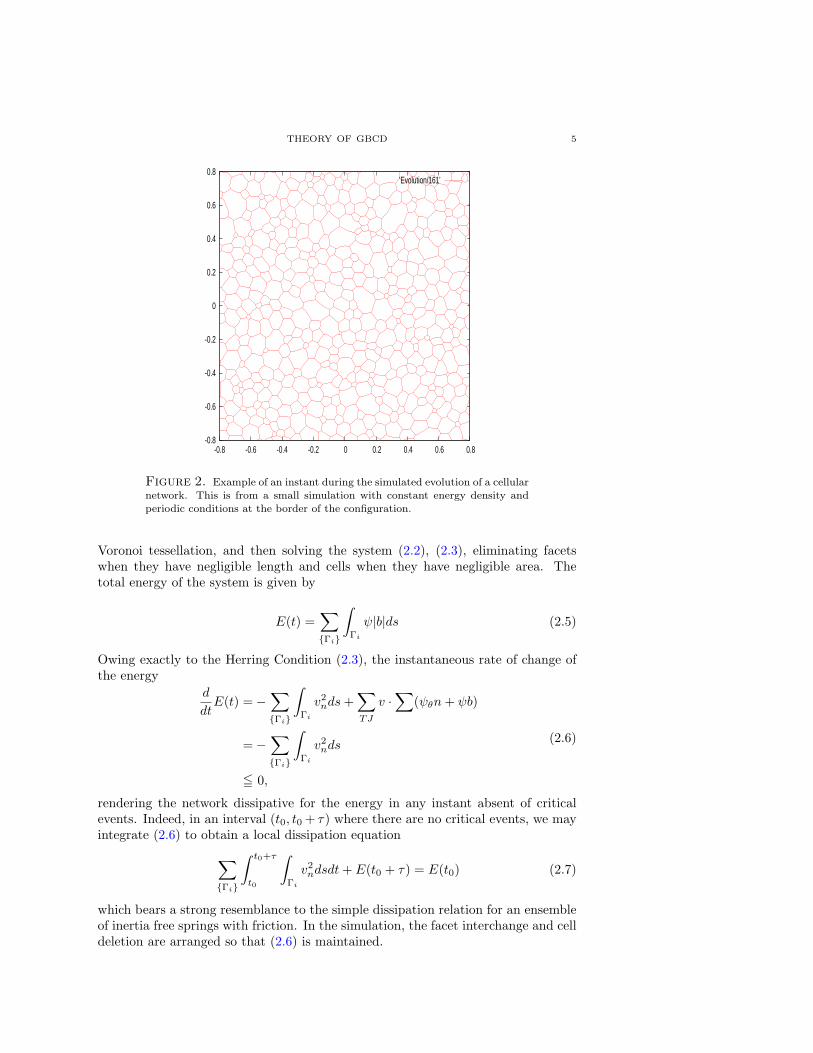
We turn now to a network of grains bounded by Γi subject to some conditionat the border of the region they occupy, like fixed end points or periodicity, cf.Figure 2. Our simulation is described in [41],[38]. The typical simulation consists ininitializing a configuration of cells and their boundary arcs, usually by a modified

THEORY OF GBCD 5

-0.8

-0.6

-0.4

-0.2

0

0.2

0.4

0.6

0.8

-0.8 -0.6 -0.4 -0.2 0 0.2 0.4 0.6 0.8

’Evolution/161’

Figure 2. Example of an instant during the simulated evolution of a cellularnetwork. This is from a small simulation with constant energy density and

periodic conditions at the border of the configuration.

Voronoi tessellation, and then solving the system (2.2), (2.3), eliminating facetswhen they have negligible length and cells when they have negligible area. Thetotal energy of the system is given by

E(t) =∑Γi

∫Γi

ψ|b|ds (2.5)

Owing exactly to the Herring Condition (2.3), the instantaneous rate of change ofthe energy

d

dtE(t) =−

∑Γi

∫Γi

v2nds+

∑TJ

v ·∑

(ψθn+ ψb)

=−∑Γi

∫Γi

v2nds

5 0,

(2.6)

rendering the network dissipative for the energy in any instant absent of criticalevents. Indeed, in an interval (t0, t0 + τ) where there are no critical events, we mayintegrate (2.6) to obtain a local dissipation equation∑

Γi

∫ t0+τ

t0

∫Γi

v2ndsdt+ E(t0 + τ) = E(t0) (2.7)

which bears a strong resemblance to the simple dissipation relation for an ensembleof inertia free springs with friction. In the simulation, the facet interchange and celldeletion are arranged so that (2.6) is maintained.


Suppose, for simplicity, that the energy density is independent of the normaldirection, so ψ = ψ(α). It is this situation that will concern us here. Then (2.2)and (2.3) may be expressed

vn = ψκ on Γ (2.8)∑i=1,...,3

ψb(i) = 0 at p, (2.9)

where p denotes a triple junction. (2.9) is the same as the Young wetting law. Ourinterfacial energy densities ψ are chosen so that

1 5 ψ(α) 532, |α| 5 π

4, (2.10)

(periodic with period π/2) giving square symmetry which is intended to mimic cubicsymmetry in three dimensions. For the range of ψ in (2.10), one may check that(2.9) can always be resolved, namely, given three numbers ψi ∈ [1, 3/2] there areunit vectors bi such that

ψ1b1 + ψ2b2 + ψ3b3 = 0.In executing this check, one may see that if the oscillation in ψ is too large, then itmay not be possible to fulfill the Young Law condition in general. In practice, wehave found the energy anisotropy to be less than 20%. Perhaps it is also of valueto point out, in this context, that the failure of all but one cell to evacuate thenetwork under (2.10) cannot be attributed to incompatibility but is likely due toconfigurational hinderance or near equilibrium behavior.

For this situation we define the grain boundary character distribution, GBCD,

ρ(α, t) = relative length of arc of misorientation α at time t,

normalized so that∫

Ω

ρdα = 1.(2.11)

3. Discussion of the Simulation. The simulation of evolution is based on solvingnumerically the system (2.2), (2.3) for the network while managing the criticalevents. It must be designed so it is robust and reliable statistics can be harvested.Owing to the size and complexity of the network there are number of challenges inthe designing of the method. These include• management of the data structure of cells, facets, and triple junctions, dy-

namic because of critical events,• management of the computational domain• initialization of the computation,• maintaining the triple junction boundary condition (2.3) while• resolving the equations (2.2) with sufficient accuracy

We will address some of these issues below. We also need some diagnostics to un-derstand accuracy. For example, it is known that the average area of cells growslinearly even in very casual simulations of coarsening, although more careful diag-nostics show that the Herring Condition (2.3) fails. As noted in the introduction,this will lead to an unreliable determination of the GBCD.In view of the dissipation inequality (2.6) the evolution of the grain boundary sys-tem may be viewed as a modified steepest descent for the energy. Therefore, thecornerstone of our scheme which assures its stability is the discrete dissipation in-equality for the total grain boundary energy which holds when the discrete HerringCondition is satisfied.

THEORY OF GBCD 7

In general, discrete dissipation principles ensure the stability and convergence ofnumerical schemes to the continuous solution. Here we work with a weak formu-lation, a variational principle, to avoid the additional complexity of higher orderspaces. It is not necessary to know the normal direction, nor is there explicit use ofcurvature.

Let us address now some details of the more important features related to thedesign and implementation of the scheme. The data structure for the execution ofthe simulation consists of the lists of the cells - grains, edges - grain boundariesand vertices - triple junctions. These lists communicate with each other duringsimulation and are managed using standard linked-lists: each grain boundary haspointers to the two grains sharing it as a boundary, each boundary also has pointersto its end points, triple junctions. Each triple junction has pointers to three grainboundaries that meet at that point. Each grain has pointers to a list of its grainboundaries.We initialize a configuration of cells and their boundary arcs, by a Voronoi diagramwith N0 seeds place randomly in the computational domain and we impose ‘periodicboundary conditions’ on the boundary of the domain. We would like to emphasizethat we do not work with functions which have periodic boundary conditions butwith cell structures which mirror each other near the borders and it must be dy-namically updated. This is an important part of the algorithm and it is necessaryso the statistics will always sample in the same computational domain.

Each cell is assigned an orientation and the misorientation parameter of a bound-ary is the difference of the orientations of the grains which share it. Typically theorientations are normally distributed, so the misorientations are also normally dis-tributed.

The simulation of the grain network is done in three steps by evolving firstthe grain boundaries, according to Mullin’s equation, and then updating the triplepoints according to Herring’s boundary condition (2.3) , imposed at the triple junc-tions, and finally managing the rearrangement events. In our numerical simulations,grain boundaries are defined by the set of nodal points and are approximated usinglinear elements. In the algorithm, we define a global mesh size, h, and uniformlydiscretized grain boundaries with local mesh size (distance between neighboringnodal points) which depends on h. Due to the frequency of critical events, we haveused a first order method in time, namely the Forward Euler method. Increasingthe order of time discretization to 2 by using a predictor corrector method did notaffect the distribution functions, which is the focus of this study.Resolution of the Herring Condition: To satisfy the Herring Condition (2.3) one hasto solve the nonlinear equation to determine the new position of the triple junction[41]. We use Newton’s method with line search [35] to approximate the new posi-tion for the triple junction. As the initial guess for Newton’s method, we determinethe position of the triple point by defining the velocity of the triple junction to beproportional to the total line stress at that point with coefficient of the proportion-ality equal to the mobility. This is also dissipative for the network. The Newtonalgorithm stops if it exceeds a certain tolerance on the number of the iterations. Ifthe Newton’s algorithm converges, the Herring Condition (2.3) is satisfied with themachine precision accuracy at the new position of the triple junction. If Newton’salgorithm fails to converge at some triple junctions (this happens when we workwith very small cells) we use our initial guess to update its position.


Critical events: As grain growth proceeds, critical events occur. When grain bound-aries (GB) shrink below a certain size, they trigger one or more of the followingprocesses (i) short GB removal, (ii) splitting of unstable junctions (where more thenthree GB meet) (ii) fixing double GB (GB that share two vertices).Removal of short GB: A short GB whose length is decreasing is removed. If itslength is increasing, it is not removed.Splitting unstable vertices: When a GB disappears, new vertices may appear wheremore than three edges meet. These are unstable and split, introducing a new vertexand a new GB of short length, reducing the number of edges meeting at the unstablejunctions. This process continues until all vertices are triple junctions. Details ofeach split are designed to maximally decrease the energy.

4. Simplified coarsening model. A significant difficulty in developing a theoryfor the GBCD, and understanding texture development in general, lies in the lackof understanding of consequences of rearrangement events or critical events, facetinterchange and grain deletion, on misorientations and grain size. For example, inFig. 3, the average area of five-faceted grains during a growth experiment on anAl thin film and the average area of five-faceted cells in a typical simulation bothincrease with time. Now the von Neumann-Mullins Rule is that the area An of acell with n-facets satisfies

A′n(t) = c(n− 6),when ψ = const. and hence triple junctions meet at angles of 2π/3. This is thoughtto hold approximately when anisotropy is small. The von Neumann-Mullins Ruledoes not fail in the example above, of course, but cells observed at later times had6, 7, 8, ... facets at earlier times. Thus in the network setting, changes whichrearrange the network play a major role. Although we may be reasonably confidentthat small cells with a small number of facets will be deleted, their resulting effecton the configuration appears to be essentially random.

Figure 3. Average area of five-sided cell populations in (a) an experiment

on Al thin film and (b) a typical simulation.

We shall approach this by a simplified model which retains kinetics and criticalevents but neglects curvature driven growth of the boundaries. It is an abstraction

THEORY OF GBCD 9

of the role of triple junctions in the presence of the rearrangement events. We haveused this model to develop a statistical theory for critical events, [12],[13],[11]. Ithas been found to have its own GBCD which we shall now study.

Our theme will be that the GBCD statistic for the simplified problem resemblesthe solution of a Fokker-Planck Equation via the mass transport implicit scheme,[37]. The first part of the discussion consists in introducing this model. The simpli-fied model is formulated as a gradient flow which results in a dissipation inequalityanalogous to the one found for the coarsening grain network. Because of this sim-plicity, it will be possible to ‘upscale’ the network level system description to ahigher level GBCD description that accomodates irreversibility. As this changesthe ensemble, there is an entropic contribution, which we take in the form of con-figurational entropy. A more useful dissipation inequality is obtained by modifyingthe viscous term to be a mass transport term, which now brings us to the realm ofthe Kantorovich-Rubenstein-Wasserstein implicit scheme. This then suggests theFokker-Planck paradigm.

The second part of the discussion, in section 5, will be our argument to validatethis paradigm. We do not know the the statistic solves the Fokker-Planck PDE butwe ask if it shares important aspects of Fokker-Planck behavior. We give evidencefor this by asking for the unique ‘temperature’ parameter that minimizes the rela-tive entropy over long time. The empirical stationary distribution and Boltzmanndistribution with the special value of ‘temperature’ are in excellent agreement, Fig-ure 6. This gives an explanation for the stationary distribution and the kinetics ofevolution. We do not know, at this point in time, that the two dimensional net-work has the detailed dissipative structure of the simplified model, but we are ableto produce evidence that the same argument employing the relative entropy doessuggest the correct kinetics and stationary distribution.

4.1. Formulation. Let I ⊂ R be an interval of length L partitioned by pointsxi, i = 1, . . . , n, where xi < xi+1, i = 1, . . . , n − 1 and xn+1 identified with x1.For each interval [xi, xi+1], i = 1, . . . , n select a random misorientation numberαi ∈ (−π/4, π/4]. The intervals [xi, xi+1] correspond to grain boundaries withmisorientations αi and the points xi represent the triple junctions. Choose anenergy density ψ(α) = 0 and introduce the energy

E =∑

i=1,...,n

ψ(αi)(xi+1 − xi). (4.1)

We impose gradient flow kinetics with respect to (4.1), which is the system ofordinary differential equations

dxidt

= − ∂E∂xi

, i = 1, ..., n, that is

dxidt

= ψ(αi)− ψ(αi−1), i = 2...n, anddx1

dt= ψ(α1)− ψ(αn).

(4.2)

The velocity vi of the ith boundary is

vi =dxi+1

dt− dxi

dt= ψ(αi−1)− 2ψ(αi) + ψ(αi+1). (4.3)

The grain boundary velocities are constant until one of the boundaries collapses.That segment is removed from the list of current grain boundaries and the velocitiesof its two neighbors are changed due to the emergence of a new junction. Each suchdeletion event rearranges the network and, therefore, affects its subsequent evolution


just as in the two dimensional cellular network. Actually, since the interval velocitiesare constant, this gradient flow is just a sorting problem. At any time, the nextdeletion event occurs at smallest of

xi − xi+1

vi.

The length li(t) of the ith interval is linear until it reaches 0 or until a collisionevent, when it becomes linear with a different slope. In any event, it is continuous,so E(t), t > 0, the sum of such functions multiplied by factors, is continuous.

We turn now to the dissipation inequality for the gradient flow. At any time tbetween deletion events,

dE

dt=∑

ψ(αi)vi

= −∑

(ψ(αi)− ψ(αi−1))2

= −∑ dxi

dt

2

5 0.

(4.4)

Suppose that the segment [xc, xc+1] is deleted at time tc, so vc < 0 for t < tc andnear it. Now

E(t) >∑i6=c

ψ(αi)li(t), for t < tc

and soE(tc) = lim

t→t+c

∑i 6=c

ψ(αi)li(t) 5 limt→t−c

E(t)

Thus E(t) is continuous decreasing Lipschitz (piecewise linear) with derivative givenby (4.4) a.e.. We may write a mass-spring-dashpot-like local dissipation inequalityanalogous to the grain growth one. In an interval (t0, t0 + τ) where there are nocritical events, dE/dt may be integrated to give

τ∑i=1...n

dxidt

2

+ E(t0 + τ) = E(t0)

or ∑i=1...n

∫ τ

0

dxidt

2

dt+ E(t0 + τ) = E(t0) (4.5)

With appropriate interpretation of the sum, (4.5) holds for all t0 and almost everyτ sufficiently small. With the obvious use of Young’s Inequality, we have that

14

∑i=1...n

∫ τ

0

v2i dt+ E(t0 + τ) 5 E(t0) (4.6)

The energy of the system at time t0 + τ is determined by its state at time t0. Viceversa, changing the sign on the right hand side of (4.2) allows us to begin with thestate at time t0 + τ and return to the state of time t0: the system is reversible inan interval of time absent of rearragement events. This is no longer the situationafter such an event. At the later time, we have no knowledge about which interval,now no longer in the inventory, was deleted.

We introduce a new ensemble based on the misorientation parameter α wherewe take Ω : −π4 5 α 5 π

4 , for later ease of comparison with the two dimensionalnetwork for which we are imposing “cubic” symmetry, i.e., “square” symmetry inthe plane. The GBCD or character distribution in this context is, as expected,

THEORY OF GBCD 11

the histogram of lengths of intervals sorted by misorientation α scaled to be aprobability distribution on Ω. To be precise, let

li(α, t) = xi+1(t)− xi(t)

= length of the ith interval, where explicit note has been taken ofits misorientation parameter α

Now partition Ω into m subintervals of length h = π2

1m and let

ρ(α, t) =∑

α′∈((k−1)h,kh]

li(α′, t) ·1Lh

, for (k − 1)h < α 5 kh. (4.7)

For this definition of the statistic,∫Ω

ρ(α, t)dα = 1

Let us make a reasonable estimate of∂ρ

∂t(α, t) =

∑α′∈((k−1)h,kh]

vi(α′) ·1Lh

, for (k − 1)h < α 5 kh. (4.8)

Generally speaking suppose that there are M data points in the sample and thatthis number is approximately the same throughout the simulation and they areuniformly distributed in the m bins. The approximate number of items of data ineach box is given by

]l(α′, t) = M · 1m

=2π·Mh

Hence, using Schwarz, as more or less a good guess,

|∂ρ∂t

(α, t)|2 5 (1Lh

)2∑

α′∈((k−1)h,kh]

v2i · ]l(α′, t)

=2MπL2

∑α′∈((k−1)h,kh]

v2i

1h, for (k − 1)h < α 5 kh,

whence integrating over Ω, that is summing over all the intervals ((k−1)h, kh], k =1, . . . ,m, ∫

Ω

|∂ρ∂t

(α, t)|2dα 5∑

k=1,...,m

2MπL2

∑α′∈((k−1)h,kh]

v2i

1h· h,

52MπL2

∑i

v2i

(4.9)

The right hand side of (4.9)2 is bounded in terms of initial parameters.Note that

E(t) =∑

ψ(αi) ·1Lh

li(αi, t) · Lh = L

∫Ω

ψ(α)ρ(α, t)dα,

where an O(h) term has been neglected.We may express (4.6) in terms of the character distribution (4.7), which amounts

to

µ0

∫ t0+τ

t0

∫Ω

|∂ρ∂t

(α, t)|2dαdt+∫

Ω

ψ(α)ρ(α, t0 + τ)dα 5∫

Ω

ψ(α)ρ(α, t0)dα, (4.10)

where µ0 > 0 is some constant.


We now impose a modeling assumption. The expression (4.10) is in terms ofthe new misorientation level ensemble, upscaled from the local level of the originalsystem, and, consistent with the lack of reversibility when rearrangement eventsoccur, an entropic term will be added. We use standard configurational entropy,

+∫

Ω

ρ log ρdα, (4.11)

although this is not the only choice. Minimizing (4.11) favors the uniform state,which would be the situation were ψ(α) = constant.

Given that (4.10) holds, we assume that for any t0 and τ sufficiently small that

µ0

∫ t0+τ

t0

∫Ω

(∂ρ

∂t)2dαdt+

∫Ω

(ψρ+ λρ log ρ)dα|t0+τ 5∫

Ω

(ψρ+ λρ log ρ)dα|t0(4.12)

E(t) was analogous to an internal energy or the energy of a microcanonical ensembleand now

F (ρ) = Fλ(ρ) = E(t) + λ

∫Ω

ρ log ρdα (4.13)

is a free energy.

4.2. Mass transport paradigm. Let us first briefly review the notion of Kantorovich-Rubenstein-Wasserstein metric, or simply Wasserstein metric, and some known re-sults that will be used in our analysis below. The reader can consult [59], [3] formore detailed exposition of the subject.

Let D ⊂ R be an interval, perhaps infinite, and f∗, f a pair of probability densi-ties on D (with finite variance). The quadratic Wasserstein metric or 2-Wassersteinmetric is defined to be

d(f, f∗)2 = infP

∫D

|x− y|2dp(x, y)

P = joint distributions for f, f∗ on D × D,(4.14)

i.e., the marginals of any p ∈ P are f, f∗. The metric induces the weak-∗ topologyon C(D)′. If f, f∗ are strictly positive, there is a transfer map which realizes p,essentially the solution of the Monge-Kantorovich mass transfer problem for thissituation. This means that there is a strictly increasing

φ : D → D such that∫D

ζ(y)f(y)dy =∫D

ζ(φ(x))f∗(x)dx, ζ ∈ C(D), and

d(f, f∗)2 =∫D

|x− φ(x)|2f∗dx

(4.15)

In this one dimensional situation, as was known to Frechet, [24],

φ(x) = F ∗−1(F (x)), x ∈ D,where

F ∗(x) =∫ x

−∞f∗(x′)dx′ and F (x) =

∫ x

−∞f(x′)dx′

(4.16)

THEORY OF GBCD 13

are the distribution functions of f∗, f . In one dimension there is only one transfermap. Finally, by a result of Benamou and Brenier [15],

1τd(f, f∗)2 = inf

∫ τ

0

∫D

v2fdξdt

over deformation paths f(ξ, t) subject to

ft + (vf)ξ = 0, (continuity equation)

f(ξ, 0) = f∗(ξ), f(ξ, τ) = f(ξ) (initial and terminal conditions)

(4.17)

The conditions (4.17) are in ‘Eulerian’ form. Likewise there is the ‘Lagrangian’ formwhich follows by rewriting (4.17) using the transfer function formulation in (4.15),

1τd(f, f∗)2 = inf

∫ τ

0

∫D

φ2tf∗dx

over transfer paths φ(x, t) from D to D with

φ(x, 0) = x and φ(x, τ) = φ(x)

(4.18)

Now let us go back and consider the inequality (4.12) above. This energy in-equality fails as a proper dissipation principle because the first term

µ0

∫ t0+τ

t0

∫Ω

(∂ρ

∂t)2dαdt

does not represent lost energy due to frictional or viscous forces. For a deformationpath f(α, t), t0 5 t 5 t0 + τ, of probability densities, this quantity is∫ τ

0

∫Ω

v2fdαdt (4.19)

where f, v are related by the continuity equation and initial and terminal conditions

ft + (vf)α = 0 in Ω× (t0, t0 + τ), and

f(α, t0) = ρ(α, t0), f(α, t0 + τ) = ρ(α, t0 + τ),(4.20)

by analogy with fluids [43], p.53 et seq., and elementary mechanics.Therefore, our goal is to replace the expression (here we denote the starting timet0 by 0) ∫ τ

0

∫Ω

(∂ρ

∂t)2dαdt (4.21)

in (4.5) or (4.13) by a proper dissipation term, eg. (4.19) and subseqently by theWasserstein metric introduced above. Since they induce different topologies onprobability densities, an inequality where (4.21) dominates (4.14) will involve termsother than the two metrics themselves.

Let us proceed as follows. Let Ω be a bounded interval, say Ω = (0, 1). Assumethat our statistic ρ(α, t) satisfies

ρ(α, t) = δ > 0 in Ω, t > 0. (4.22)

This is a necessary assuption for our estimates below. In fact, to proceed withthe implicit scheme introduced later, it is sufficient to require (4.22) just for theinitial data ρ0(α) since this property is inherited by the iterates. We now use the


representation (4.17) and we use the deformation path given by ρ itself to calculatethat for some cΩ > 0,

1τd(ρ, ρ∗)2 5

∫ τ

0

∫Ω

v2ρdxdt 5cΩ

minΩ ρ

∫ τ

0

∫Ω

∂ρ

∂t(x, t)2dxdt,

ρ∗(x) = ρ(x, 0) and ρ(x) = ρ(x, τ),(4.23)

where 0 represents an arbitrary starting time and τ a relaxation time. Given thepair (v, ρ), integrate the continuity equation in (4.17) to obtain the non-conservativeform

∂F

∂t+ v

∂F

∂x=∂F

∂t+ vρ = c in Ω, 0 < t < τ.

Now Ft|∂Ω = 0 and v|∂Ω = 0 for 0 < t < τ , so the possibly time dependent constantabove vanishes. Thus

v2ρ(x, t) =Ft(x, t)2

ρ(x, t)5

x

ρ(x, t)

∫Ω

ρt(y, t)2dy, x ∈ Ω, 0 < t < τ (4.24)

Integrating (4.24),∫ τ

0

∫Ω

v2ρdxdt 5∫ τ

0

∫Ω

x

ρ(x, t)dx

∫Ω

ρt(y, t)2dydt

5cΩ

minΩ ρ·∫ τ

0

∫Ω

ρt(y, t)2dydt.

(4.25)

Thus, again keeping (4.17) in mind,

1τd(ρ, ρ∗)2 = inf

∫ τ

0

∫Ω

v2ρdξdt 5cΩ

minΩ ρ·∫ τ

0

∫Ω

ρt(y, t)2dydt. (4.26)

Hence, in view of (4.26), we obtain (4.23).We then find that there is a µ > 0 such that for any relaxation time τ > 0,

µ

2

∫ τ

0

∫Ω

v2ρdαdt+ Fλ(ρ) 5 Fλ(ρ∗) (4.27)

We next replace (4.27) by a minimum principle, arguing that the path givenby ρ(α, t) is the one most likely to occur and the minimizing path has the highestprobability. For this step, let ρ∗ = ρ(·, t0) and ρ = ρ(·, t + τ). Observe that from(4.17),

1τd(ρ, ρ∗)2 = inf

∫ τ

0

∫Ω

v2fdαdt

over deformation paths f(α, t) subject to

ft + (vf)α = 0, (continuity equation)

f(ξ, 0) = ρ∗(α), f(α, τ) = ρ(α, τ) (initial and terminal conditions)

(4.28)

where d is the Wasserstein metric. So we may express the minimum principle inthe form

µ

2τd(ρ, ρ∗)2 + Fλ(ρ) = inf µ

2τd(η, ρ∗)2 + Fλ(η) (4.29)

For each relaxation time τ > 0 we determine iteratively the sequence ρ(k) bychoosing ρ∗ = ρ(k−1) and ρ(k) = ρ in (4.29) and set

ρ(τ)(α, t) = ρ(k)(α) in Ω for kτ 5 t < (k + 1)τ. (4.30)

THEORY OF GBCD 15

We then anticipate recovering the GBCD ρ as

ρ(α, t) = limτ→0

ρ(τ)(α, t), (4.31)

with the limit taken in a suitable sense. It is known for some time that ρ obtainedfrom (4.31) is the solution of the Fokker-Planck Equation, [37] or see Appendix 8.1for the brief description.

µ∂ρ

∂t=

∂

∂α(λ∂ρ

∂α+ ψ′ρ) in Ω, 0 < t <∞. (4.32)

We might point out here, as well, that a solution of (4.32) with periodic boundaryconditions and nonnegative initial data is positive for t > 0.

5. Validation of the scheme. We now begin the validation step of our model.Introduce the notation for the Boltzmann distribution with parameter λ

ρλ(α) =1Zλ

e−ψ(α)λ , α ∈ Ω, with Zλ =

∫Ω

e−ψ(α)λ dα. (5.1)

As outlined in Appendix 8.2, with validation we would gain qualitative propertiesof solutions of (4.32):

• ρ(α, t)→ ρλ(α) as t→∞, and• this convergence is exponentially fast.

The Kullback-Leibler relative entropy for (4.32) is given by

Φλ(η) = λ

∫Ω

η logη

ρλdα where

η = 0 in Ω,∫

Ω

ηdα = 1,(5.2)

with ρλ from (5.1). By Jensen’s Inequality it is always nonnegative. In terms ofthe free energy (4.13) and (5.1), (5.2) is given by

Φλ(η) = Fλ(η) + λ logZλ. (5.3)

The procedure which leads to the implicit scheme, based on the dissipation in-equality (4.6), holds for the entire system but does not identify individual intermedi-ate ‘spring-mass-dashpots’. The consequence is that we cannot set the temperature-like parameter σ, but in some way must decide if one exists. Therefore, we seek toidentify the particular λ = σ for which Φσ defined by the GBCD statistic ρ tendsmonotonely to the minimum of all the Φλ as t becomes large. We then ask if theterminal, or equilibrium, empirical distribution ρ is equal to ρσ. For our purposes,we simply decide the question of equality by inspection.

In this context, deciding a parameter on the basis of its thermodynamic restric-tions is employed in [17],[18],[19] and recalls the Coleman-Noll procedure.

To understand our implementation, we offer an illustration using the solution ofthe (4.32) itself, u computed on Ω = (0, 1) with the choice λ = σ = 0.0296915,and a collection of relative entropy plots Φλ where values of λ are close to σ, cf.Figure 4(left). The plot of Φσ vs. time t is noted in red and it is decreasing andtends to 0. A glance at the resulting equilibrium u, Figure 4(right), identifies it asthe Boltzmann distribution ρσ, as constructed.


Figure 4. (left) The relative entropy Φσ of the solution u(x, t) of the Fokker-

Planck Equation (4.32) for the potential ψ(x) = 1 + r(x− 12

)2, r = 2, with thechoice λ = σ = 0.0296915, computed by a routine numerical method, compared

with a sequence of Φλ with the curve for σ = 0.0296915 noted in red. The

values of λ correspond to ρλ with max ρσ/2 5 max ρλ 5 (3/2) max ρσ (right)The computed equlibrium solution, which is indistinguishable from ρσ , the

Boltzmann distribution of (5.2).

Figure 5. Plots of − log Φλ vs. t with − log Φσ in red. Plot illustrates that

Φσ decreases exponentially to 0 but that Φλ for choices of λ 6= σ do not have

this property.

For the simplified coarsening model, we consider

ψ(α) = 1 + 2α2 in Ω = (−π4,π

4), (5.4)

and shall identify a unique such parameter, which we label σ, by seeking the min-imum of the relative entropy (5.2) and then comparing it with ρσ. This ψ thedevelopment to second order of ψ(α) = 1 + 0.5 sin2 2α used in the 2D simulation.Moreover, since the potential is quadratic, it represents a version of the Ornstein-Uhlenbeck process. To proceed, we must agree upon which time T∞ represents time

THEORY OF GBCD 17

equals infinity. For the simplified critical event model we are considering, it is clearthat by computing for a sufficiently long time, all cells will be gone. This time maybe quite long. We choose the time parameter so that 80% of segments have beendeleted, which corresponds to the stationary configuration in the two-dimensionalsimulation. For the simplifed model simulation, this time is T (80%) = 6.73. Forcomparison, T (90%) = 30 and T (95%) =103. There may be additional criteria forchoosing a T in the neighborhood of T (80%) and we may wish to discuss this later.

This simulation is initialized with 215 + 1 cells and approximately 155 trial dis-tributions ρj are collected at 200 rearrangement event intervals. 155 trial relativeentropies are constructed from gaussians ρλj satisfying

ρλj (0) = max ρλj = max ρj . (5.5)

A selection of these are shown in Figure 6. We include the collection of plots of

Figure 6. Graphical results for the simplified coarsening model. (left) Rel-

ative entropy plots for values of λ chosen according to (5.5) with Φσ noted

in red. The value of σ = 0.0296915. (right) Empirical distribution at timeT = T∞ in red compared with ρσ in black.

log Φλ which suggests that Φσ decays exponentially to its minimum whereas a Φλcorresponding to a subsequent empirical distribution does not.

For a second example to illustrate the method, we consider the potential

ψ(α) = 1 + εα4, −π4

5 α 5π

4, ε = 8. (5.6)

This choice, ε = 8, corresponds to the first order terms in the two dimensionalquartic energy density we discuss in the next section.

6. The entropy method for the GBCD. We shall apply the method of Section5 to the GBCD harvested from the 2D simulation. We consider first a typicalsimulation with the energy density

ψ(α) = 1 + ε(sin 2α)2, −π4

5 α 5π

4, ε = 1/2, (6.1)


Figure 7. Plots of − log Φλ vs. t with − log Φσ , σ = 0.0296915, in red for

the simplified coarsening model. It shows that Φσ decays exponentially to its

minimum at time T∞. Φλ with λ = 0.01375688608 in black does not seem tohave this property of exponential decay.

Figure 8. Graphical results for the simplfied coarsening model with poten-

tial (5.6). (left) Relative entropy plot for selected values of λ with Φσ noted inred. The value of σ = 0.003033356683 and is ascertained at the time T = T∞corresponding to 80% of cells deleted. (right) Empirical distribution at time

T = T∞ in red compared with ρσ in black.

Figure 9, initialized with 104 cells and normally distributed misorientation anglesand terminated when 2000 cells remain. At this stage, the simulation is essentiallystagnant. Possible ‘temperature’ parameters λ are constructed similarly to thoseof the simplified coarsening model. From the maximum of a harvested GBCD, weconstruct the gaussian with the same maximum. This determines a value of λ whichis used to define ρλ in (5.1) for the density (6.1). This ρλ then defines a trial relativeentropy via (5.2).

THEORY OF GBCD 19

Figure 9. The energy density ψ(α) = 1 + ε sin2 2α, |α| < π/4, ε = 12.

Figure 10. (a) The relative entropy of the grain growth simulation withenergy density (6.1) for a sequence of Φλ vs. t with the optimal choice σ ≈ 0.1

noted in red. (b) Comparison of the empirical distribution at time t = 2, when

80% of the cells have been deleted, with ρσ , the Boltzmann distribution of

(5.1).

We now identify the parameter σ, which turns out to be σ ≈ 0.1, Figure 10.From Figure 11, we see that this relative entropy Φσ has exponential decay untilit reaches a value of about 1.5, when it remains constant. The solution itself thentends exponentially in L1 to its limit ρσ by the Kullback-Leibler Inequality.

A second example presented here is a quartic energy

ψ(α) = 1 + ε(sin 2α)4, −π4

5 α 5π

4, ε = 1/2. (6.2)

Again, a configuration of 104 cells is initialized with normally distributed misori-entations and, this time, the computation proceeds until about 1000 cells remain.


Figure 11. Plot of − log Φσ vs. t with energy density (6.1). It is approxi-

mately linear until it becomes constant showing that Φσ decays exponentially

Figure 12. GBCD (red) and Boltzmann distribution (black) for the po-tential ψ of (6.1) with parameter σ ≈ 0.1 as predicted by our theory. This

GBCD is averaged over 5 trials.

The relative entropy and the equilibrium Boltzmann statistic stabilize when 2000cells remain.

With the equilibrium solution in hand, as depicted in Figure 13, we again ini-tialized a configuration of 104 cells with, on this occasion, misorientations normallydistributed in the much narrower range defined by the sides of the solution GBCD.Since these misorientations see, essentially, only the near minimum of the potential,we would expect the new stationary distribution to be gaussian or random. How-ever we obtain the same relative entropy curve and equilibrium depicted in Figure13. Although this is not like a molecular system with eternal collisions causingthe entire system to equilibrate, the fluctuations of misorientations caused by the

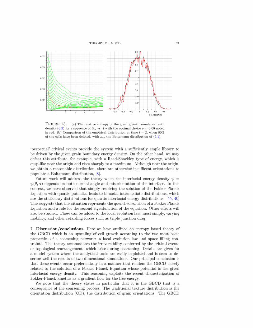
THEORY OF GBCD 21

Figure 13. (a) The relative entropy of the grain growth simulation with

density (6.2) for a sequence of Φλ vs. t with the optimal choice σ ≈ 0.08 notedin red. (b) Comparison of the empirical distribution at time t = 2, when 80%

of the cells have been deleted, with ρσ , the Boltzmann distribution of (5.1).

‘perpetual’ critical events provide the system with a sufficiently ample library tobe driven by the given grain boundary energy density. On the other hand, we maydefeat this attribute, for example, with a Read-Shockley type of energy, which iscusp-like near the origin and rises sharply to a maximum. Although near the origin,we obtain a reasonable distribution, there are otherwise insufficent orientations topopulate a Boltzmann distribution, [8].

Future work will address the theory when the interfacial energy density ψ =ψ(θ, α) depends on both normal angle and misorientation of the interface. In thiscontext, we have observed that simply resolving the solution of the Fokker-PlanckEquation with quartic potential leads to bimodal intermediate distributions, whichare the stationary distributions for quartic interfacial energy distributions. [55, 40]This suggests that this situation represents the quenched solution of a Fokker PlanckEquation and a role for the second eigenfunction of the equation. Other effects willalso be studied. These can be added to the local evolution law, most simply, varyingmobility, and other retarding forces such as triple junction drag.

7. Discussion/conclusions. Here we have outlined an entropy based theory ofthe GBCD which is an upscaling of cell growth according to the two most basicproperties of a coarsening network: a local evolution law and space filling con-traints. The theory accomodates the irreversibility conferred by the critical eventsor topological rearrangements which arise during coarsening. Details are given fora model system where the analytical tools are easily exploited and is seen to de-scribe well the results of two dimensional simulations. Our principal conclusion isthat these events occur preferentially in a manner that renders the GBCD closelyrelated to the solution of a Fokker Planck Equation whose potential is the giveninterfacial energy density. This reasoning exploits the recent characterization ofFokker-Planck kinetics as a gradient flow for the free energy.

We note that the theory states in particular that it is the GBCD that is aconsequence of the coarsening process. The traditional texture distribution is theorientation distribution (OD), the distribution of grain orientations. The GBCD


is the distribution of differences of the OD, basically the convolution of the ODwith itself. This relationship may be inverted, by elementary Fourier analysis, so,in this simple case, the GBCD determines the OD and not the other way around.Therefore, we may expect, in nature, that it is among the processes that determinethe OD.

8. Appendix: The Kantorovich-Rubinstein-Wasserstein (KRW) implicitscheme for Fokker-Planck Equation and the asymptotic behavior.

8.1. The KRW implicit scheme for the Fokker-Planck Equation. The Fokker-Planck Equation is the Euler-Lagrange Equation of a gradient flow for a free energywith respect to the Wasserstein metric, [37], as is now well established. Here wegive a very brief description. Give a (smooth) potential ψ and a parameter σ > 0defined on a bounded interval Ω, for definiteness, and define the free energy definedon probability densities

F (ρ) =∫

Ω

(ψρ+ σρ log ρ)dx. (8.1)

Given initial data ρ0 and τ > 0, a relaxation time, we iteratively determine asequence ρ(k) with the procedure: set ρ(0) = ρ0 and given ρ∗ = ρ(k−1) determineρ(k) = ρ the solution of the variational problem

12τd(ρ, ρ∗)2 + F (ρ) = inf

η 1

2τd(η, ρ∗)2 + F (η),

η = probability densities on Ω subject to appropriate boundary conditions.(8.2)

Settingρ(τ)(x, t) = ρ(k)(x) for kτ 5 t < (k + 1)τ, (8.3)

the limit functionρ = lim

τ→0ρ(τ)

satisfies the Fokker-Planck Equation

∂ρ

∂t=

∂

∂x(σ∂ρ

∂x+ ψ′ρ), x ∈ Ω, t > 0, (8.4)

along with the appropriate boundary conditions, natural or periodic, and initialcondition ρ = ρ0.

A known property of the iteration procedure in (8.2) is that iterates remainpositive, indeed, bounded below, if the initial data is positive and are boundedabove. This simplifies the limiting process.

8.2. Asymptotic behavior. One of the diagnostics we consider in the analysis ofthe GBCD and the one we employ to identify the ’temperature’ parameter σ is thedecay of the relative entropy. It is straightforward to show that the relative entropytends to zero as t → ∞, and we review it below. The decay is also exponential.This is not surprising since the same is true for convergence to the stationary statefor a finite ergodic Markov chain. There are many ways to show this for (8.4).It follows from the Sturm-Liouville theory and separation of variables, [25] or theKrein-Rutman theorem. A more recent technique is to use a log-Sobolev inequality.Here we sketch an inexpensive version based on an energy estimate which does notactually require the log-Sobolev inequality.

THEORY OF GBCD 23

Let us assume throughout that ρ(x, t) is a solution of (8.4) in Ω, a boundedinterval, namely

∂ρ

∂t=

∂

∂x(σ∂ρ

∂x+ ψ′ρ), x ∈ Ω, t > 0,

σ∂ρ

∂x+ ψ′ρ = 0 on ∂Ω, t > 0,

(8.5)

or∂ρ

∂t=

∂

∂x(σ∂ρ

∂x+ ψ′ρ), x ∈ Ω, t > 0,

ρ periodic in x for t > 0.(8.6)

First we establish the adjoint equation. Let

ρ](x) =1Ze−

ψ(x)σ , x ∈ Ω, with Z =

∫Ω

e−ψ(x)σ dx, (8.7)

denote the stationary distribution for (8.5) or (8.6) For a smooth ζ,∫Ω

ρtζdx =∫

Ω

(σρx + ψ′ρ)xζdx

= −∫

Ω

(σρx + ψ′ρ)ζxdx

= −σ∫

Ω

(ρx +ψ′

σρ)ζxdx

= −σ∫

Ω

e−ψσ (e

ψσ ρ)xζxdx

(8.8)

Rewriting (8.8), we have that∫Ω

( ρρ])tζρ]dx = −σ

∫Ω

( ρρ])xζxρ

]dx. (8.9)

Sou(x, t) =

( ρρ])(x, t), a(x) = ρ](x), x ∈ Ω, t > 0

satisfies

aut = σ(aux)x, x ∈ Ω, t > 0.

(8.10)

Let ϕ(ξ) be convex, nonnegative, and consider

Φ(t) =∫

Ω

ϕ( ρρ])ρ]dx =

∫Ω

ϕ(u)adx (8.11)

and compute its derivative. We have that

Φ′(t) =d

dt

∫Ω

ϕ(u)adx

=∫

Ω

ϕ′(u)autdx

= σ

∫Ω

ϕ′(u)(aux)xdx

= −σ∫

Ω

ϕ′′(u)u2xadx < 0.

(8.12)

Thus Φ is decreasing and

Φ(0)− Φ(∞) = σ

∫ ∞0

∫Ω

ϕ′′(u)u2xadxdt < +∞


Since ϕ′′ = 0 and a is bounded below, it follows that∫Ω

ϕ′′(u)u2xadx→ 0 as t→∞. (8.13)

Choose, for example,

ϕ(ξ) =12

(ξ − 1)2. (8.14)

Then we deduce that ∫Ω

u2xadx→ 0 as t→∞, so

u→ constant = 1 as t→∞.(8.15)

This means that, up to a subsequence,

ρ(x, t)→ ρ](x) as t→∞ and

Φ(t)→ ϕ(1) as t→∞(8.16)

In particular, whenever ϕ(1) = 0, we have that Φ(∞) = 0, which holds in particularfor (8.14) and for the relative entropy, in this form given by

ϕ(ξ) = ξ log ξ. (8.17)

Our concern is the rate at which the relative entropy

Φ(t) = σ

∫Ω

u log u adx =∫

Ω

ρ logρ

ρ]dx (8.18)

tends to 0.First note the Poincare-style inequality: For ζ ∈ H1(Ω) with∫

Ω

ζadx = 0,

we have that∫Ω

ζ2adx 5 C0

∫Ω

ζ2xadx

(8.19)

Now look at

U(t) =12

∫Ω

(u− 1)2adx for which∫

Ω

(u− 1)adx = 0. (8.20)

Using (8.12) and (8.19),dU

dt= −σ

∫Ω

u2xadx

5 − σ

C0

∫Ω

(u− 1)2adx

= −2σC0U,

whenceU(t) 5 U(0)e−εt, 0 < t <∞, (8.21)

for an ε > 0. Finally consider (8.18), for which

ϕ′′(ξ) =1ξ

anddΦdt

= −σ∫

Ω

1uu2xadx. (8.22)

THEORY OF GBCD 25

Since u is bounded below, we may find a δ > 0 small enough such that

d

dt(U − δΦ) = −σ

∫Ω

u2x(1− δ

u)adx < 0, 0 < t <∞, (8.23)

and subsequently because U(∞) = Φ(∞) = 0, on integrating,

Φ(t) 51δU(t) 5

1δU(0)e−εt, 0 < t <∞. (8.24)

The parameters occuring in (8.24) are not structural to the entropy nor even to theequation itself but depend on the particular solution at hand. This notwithstanding,the result will serve as a guide to diagnostics for the GBCD statistic.

Acknowledgements. This work is an activity of the CMU Center for Excellence in Materials

Research and Innovation. This research was done while Y. Epshteyn and R. Sharp were postdoc-

toral associates at the Center for Nonlinear Analysis. We are grateful to our colleagues G. Rohrer,

A. D. Rollett, R. Schwab, and R. Suter for their collaboration.

REFERENCES

[1] B.L. Adams, D. Kinderlehrer, I. Livshits, D. Mason, W.W. Mullins, G.S. Rohrer, A.D. Rollett,

D. Saylor, S Ta’asan, and C. Wu. Extracting grain boundary energy from triple junction

measurement. Interface Science, 7:321–338, 1999.[2] BL Adams, D Kinderlehrer, WW Mullins, AD Rollett, and S Ta’asan. Extracting the relative

grain boundary free energy and mobility functions from the geometry of microstructures.

Scripta Materiala, 38(4):531–536, Jan 13 1998.[3] Luigi Ambrosio, Nicola Gigli, and Giuseppe Savare. Gradient flows in metric spaces and in

the space of probability measures. Lectures in Mathematics ETH Zurich. Birkhauser Verlag,Basel, second edition, 2008.

[4] Todd Arbogast. Implementation of a locally conservative numerical subgrid upscaling scheme

for two-phase Darcy flow. Comput. Geosci., 6(3-4):453–481, 2002. Locally conservative nu-merical methods for flow in porous media.

[5] Todd Arbogast and Heather L. Lehr. Homogenization of a Darcy-Stokes system modeling

vuggy porous media. Comput. Geosci., 10(3):291–302, 2006.[6] Matthew Balhoff, Andro Mikelic, and Mary F. Wheeler. Polynomial filtration laws for low

Reynolds number flows through porous media. Transp. Porous Media, 81(1):35–60, 2010.

[7] Matthew T. Balhoff, Sunil G. Thomas, and Mary F. Wheeler. Mortar coupling and upscalingof pore-scale models. Comput. Geosci., 12(1):15–27, 2008.

[8] K. Barmak, E. Eggeling, M. Emelianenko, Y. Epshteyn, D. Kinderlehrer, R.Sharp, and

S.Ta’asan. Predictive theory for the grain boundary character distribution. In Proc. Recrys-tallization and Grain Growth IV,, 2010.

[9] K. Barmak, E. Eggeling, M. Emelianenko, Y. Epshteyn, D. Kinderlehrer, R. Sharp, andS. Ta’asan. Critical events, entropy, and the grain boundary character distribution. Center

for Nonlinear Analysis 10-CNA-014, Carnegie Mellon University, 2010.[10] K. Barmak, E. Eggeling, M. Emelianenko, Y. Epshteyn, D. Kinderlehrer, and S. Ta’asan.

Geometric growth and character development in large metastable systems. Rendiconti diMatematica, Serie VII, 29:65–81, 2009.

[11] K. Barmak, M. Emelianenko, D. Golovaty, D. Kinderlehrer, and S. Ta’asan. On a statisticaltheory of critical events in microstructural evolution. In Proceedings CMDS 11, pages 185–194.

ENSMP Press, 2007.[12] K. Barmak, M. Emelianenko, D. Golovaty, D. Kinderlehrer, and S. Ta’asan. Towards a statis-

tical theory of texture evolution in polycrystals. SIAM Journal Sci. Comp., 30(6):3150–3169,2007.

[13] K. Barmak, M. Emelianenko, D. Golovaty, D. Kinderlehrer, and S. Ta’asan. A new perspectiveon texture evolution. International Journal on Numerical Analysis and Modeling, 5(Sp. Iss.SI):93–108, 2008.


[14] Katayun Barmak, David Kinderlehrer, Irine Livshits, and Shlomo Ta’asan. Remarks on amultiscale approach to grain growth in polycrystals. In Variational problems in materials

science, volume 68 of Progr. Nonlinear Differential Equations Appl., pages 1–11. Birkhauser,

Basel, 2006.[15] Jean-David Benamou and Yann Brenier. A computational fluid mechanics solution to the

Monge-Kantorovich mass transfer problem. Numer. Math., 84(3):375–393, 2000.[16] G. Bertotti. Hysteresis in magnetism. Academic Press, 1998.

[17] Eran Bouchbinder and J. S. Langer. Nonequilibrium thermodynamics of driven amorphous

materials. i. internal degrees of freedom and volume deformation. Physical Review E, 80(3,Part 1), Sep 2009.

[18] Eran Bouchbinder and J. S. Langer. Nonequilibrium thermodynamics of driven amorphous

materials. ii. effective-temperature theory. Physical Review E, 80(3, Part 1), Sep 2009.[19] Eran Bouchbinder and J. S. Langer. Nonequilibrium thermodynamics of driven amorphous

materials. iii. shear-transformation-zone plasticity. Physical Review E, 80(3, Part 1), Sep 2009.

[20] Lia Bronsard and Fernando Reitich. On three-phase boundary motion and the singular limitof a vector-valued Ginzburg-Landau equation. Arch. Rational Mech. Anal., 124(4):355–379,

1993.

[21] Philippe G. Ciarlet. The finite element method for elliptic problems. North-Holland PublishingCo., Amsterdam, 1978. Studies in Mathematics and its Applications, Vol. 4.

[22] Albert Cohen. A stochastic approach to coarsening of cellular networks. Multiscale Model.Simul., 8(2):463–480, 2009/10.

[23] Antonio DeSimone, Robert V. Kohn, Stefan Muller, Felix Otto, and Rudolf Schafer. Two-

dimensional modelling of soft ferromagnetic films. R. Soc. Lond. Proc. Ser. A Math. Phys.Eng. Sci., 457(2016):2983–2991, 2001.

[24] M Frechet. Sur la distance de deux lois de probabilite. Comptes Rendus de l’ Academie des

Sciences Serie I-Mathematique, 244(6):689–692, 1957.[25] Crispin Gardiner. Stochastic methods, 4th edition. Springer-Verlag, 2009.

[26] S. K. Godunov. A difference method for numerical calculation of discontinuous solutions of

the equations of hydrodynamics. Mat. Sb. (N.S.), 47 (89):271–306, 1959.[27] S. K. Godunov and V. S. Ryaben’kii. Difference schemes, volume 19 of Studies in Mathematics

and its Applications. North-Holland Publishing Co., Amsterdam, 1987. An introduction to

the underlying theory, Translated from the Russian by E. M. Gelbard.[28] J. Gruber, H. M. Miller, T. D. Hoffmann, G. S. Rohrer, and A. D. Rollett. Misorientation

texture development during grain growth. part i: Simulation and experiment. Acta Materialia,57(20):6102–6112, Dec 2009.

[29] J. Gruber, A. D. Rollett, and G. S. Rohrer. Misorientation texture development during grain

growth. part ii: Theory. Acta Materialia, 58(1):14–19, Jan 2010.[30] M. Gurtin. Thermomechanics of evolving phase boundaries in the plane. Oxford, 1993.

[31] R. Helmig. Multiphase flow and transport processes in the subsurface. Springer, 1997.[32] C. Herring. Surface tension as a motivation for sintering. In Walter E. Kingston, editor, The

Physics of Powder Metallurgy, pages 143–179. Mcgraw-Hill, New York, 1951.

[33] C. Herring. The use of classical macroscopic concepts in surface energy problems. In Robert

Gomer and Cyril Stanley Smith, editors, Structure and Properties of Solid Surfaces, pages5–81, Chicago, 1952. The University of Chicago Press. Proceedings of a conference arranged

by the National Research Council and held in September, 1952, in Lake Geneva, Wisconsin,USA.

[34] EA Holm, GN Hassold, and MA Miodownik. On misorientation distribution evolution during

anisotropic grain growth. Acta Materialia, 49(15):2981–2991, Sep 3 2001.

[35] Arieh Iserles. A first course in the numerical analysis of differential equations. CambridgeTexts in Applied Mathematics. Cambridge University Press, Cambridge, 1996.

[36] R Jordan, D Kinderlehrer, and F Otto. Free energy and the fokker-planck equation. PhysicaD, 107(2-4):265–271, Sep 1 1997.

[37] R Jordan, D Kinderlehrer, and F Otto. The variational formulation of the fokker-planck

equation. SIAM J. Math. Analysis, 29(1):1–17, Jan 1998.[38] D Kinderlehrer, J Lee, I Livshits, A Rollett, and S Ta’asan. Mesoscale simulation of grain

growth. Recrystalliztion and grain growth, pts 1 and 2, 467-470(Part 1-2):1057–1062, 2004.

[39] D Kinderlehrer and C Liu. Evolution of grain boundaries. Mathematical Models and Methodsin Applied Sciences, 11(4):713–729, Jun 2001.

THEORY OF GBCD 27

[40] D Kinderlehrer, I Livshits, GS Rohrer, S Ta’asan, and P Yu. Mesoscale simulation of theevolution of the grain boundary character distribution. Recrystallization and grain growth,

pts 1 and 2, 467-470(Part 1-2):1063–1068, 2004.

[41] David Kinderlehrer, Irene Livshits, and Shlomo Ta’asan. A variational approach to modelingand simulation of grain growth. SIAM J. Sci. Comp., 28(5):1694–1715, 2006.

[42] Robert V. Kohn and Felix Otto. Upper bounds on coarsening rates. Comm. Math. Phys.,229(3):375–395, 2002.

[43] L. D. Landau and E. M. Lifshitz. Fluid mechanics. Translated from the Russian by J. B.

Sykes and W. H. Reid. Course of Theoretical Physics, Vol. 6. Pergamon Press, London, 1959.[44] Peter D. Lax. Weak solutions of nonlinear hyperbolic equations and their numerical compu-

tation. Comm. Pure Appl. Math., 7:159–193, 1954.

[45] Peter D. Lax. Hyperbolic systems of conservation laws and the mathematical theory of shockwaves. Society for Industrial and Applied Mathematics, Philadelphia, Pa., 1973. Conference

Board of the Mathematical Sciences Regional Conference Series in Applied Mathematics, No.

11.[46] Bo Li, John Lowengrub, Andreas Ratz, and Axel Voigt. Geometric evolution laws for thin

crystalline films: modeling and numerics. Commun. Comput. Phys., 6(3):433–482, 2009.

[47] I.M. Lifshitz, E. M. and V.V. Slyozov. The kinetics of precipitation from suprsaturated solidsolutions. Journal of Physics and Chemistry of Solids, 19(1-2):35–50, 1961.

[48] John S. Lowengrub, Andreas Ratz, and Axel Voigt. Phase-field modeling of the dynamicsof multicomponent vesicles: spinodal decomposition, coarsening, budding, and fission. Phys.

Rev. E (3), 79(3):0311926, 13, 2009.

[49] MA Miodownik, P Smereka, DJ Srolovitz, and EA Holm. Scaling of dislocation cell struc-tures: diffusion in orientation space. PROCEEDINGS OF THE ROYAL SOCIETY A-

MATHEMATICAL PHYSICAL AND ENGINEERING SCIENCES, 457(2012):1807–1819,

Aug 8 2001.[50] W.W. Mullins. Solid Surface Morphologies Governed by Capillarity, pages 17–66. American

Society for Metals, Metals Park, Ohio, 1963.

[51] W.W. Mullins. On idealized 2-dimensional grain growth. Scripta Metallurgica, 22(9):1441–1444, SEP 1988.

[52] Felix Otto, Tobias Rump, and Dejan Slepcev. Coarsening rates for a droplet model: rigorous

upper bounds. SIAM J. Math. Anal., 38(2):503–529 (electronic), 2006.[53] GS Rohrer. Influence of interface anisotropy on grain growth and coarsening. Annual Review

of Materials Research, 35:99–126, 2005.[54] Anthony D. Rollett, S.-B. Lee, R. Campman, and G. S. Rohrer. Three-dimensional charac-

terization of microstructure by electron back-scatter diffraction. Annual Review of Materials

Research, 37:627–658, 2007.[55] DM Saylor, A Morawiec, and GS Rohrer. The relative free energies of grain boundaries in

magnesia as a function of five macroscopic parameters. Acta Materialia, 51(13):3675–3686,AUG 1 2003.

[56] Cyril Stanley Smith. Grain shapes and other metallurgical applications of topology. In Metal

Interfaces, pages 65–108, Cleveland, Ohio, 1952. American Society for Metals, American

Society for Metals.[57] H. Bruce Stewart and Burton Wendroff. Two-phase flow: models and methods. J. Comput.

Phys., 56(3):363–409, 1984.[58] Andrea Toselli and Olof Widlund. Domain decomposition methods—algorithms and theory,

volume 34 of Springer Series in Computational Mathematics. Springer-Verlag, Berlin, 2005.

[59] Cedric Villani. Topics in optimal transportation, volume 58 of Graduate Studies in Mathe-

matics. American Mathematical Society, Providence, RI, 2003.[60] J. Von Neumann and R. D. Richtmyer. A method for the numerical calculation of hydrody-

namic shocks. J. Appl. Phys., 21:232–237, 1950.[61] C Wagner. Theorie der alterung von niederschlagen durch umlosen (Ostwald-Reifung).

Zeitschrift fur Elektrochemie, 65(7-8):581–591, 1961.

Received xxxx 20xx; revised xxxx 20xx.


E-mail address: [email protected]







an entropy based theory of the grain boundary …math.gmu.edu/~memelian/pubs/pdfs/dcdsb_2010.pdf ·...

Documents