an engineer’s guide to matlab 3rd edition chapter 7 3d graphics

Copyright © Edward B. Magrab 2009

Chapter 7

1

An Engineer’s Guide to MATLAB

AN ENGINEER’S GUIDE TO MATLAB

3rd Edition

CHAPTER 7

3D GRAPHICS


Chapter 7

2


Chapter 7 – Objective

• Present the implementation of a wide selection of three-dimensional plotting capabilities.


Chapter 7

3


Topics

Lines in 3D

Surfaces


Chapter 7

4


Lines in 3D -

The 3D version of plot is

plot3(u1, v1, w1, c1, u2, v2, w2, c2,…)

where

uj, vj, and wj are the x, y, and z coordinates, respectively, of a point.

They are scalars, vectors of the same length, matrices of the same order, or expressions that, when evaluated, result in one of these three quantities.

cj is a string of characters -

One character specifies the color.

One character specifies the point characteristics.

One or two characters specify the line type.


Chapter 7

5


To draw a set of n unconnected lines whose end points are

(x1j,y1j,z1j) and (x2j,y2j,z2j), j = 1, 2, …, n

we create six vectors

1 2

1 2

2

1 2

1

j j j jn

j j j jn

j j1 j jn

x = x x … x

y = y y … y j = ,

z = z z … z

Then, plot3 is

x1 = […]; x2 = […];y1 = […]; y2 = […];z1 = […]; z2 = […]; plot3([x1; x2], [y1; y2], [z1; z2])

where [x1; x2], [y1; y2], and [z1; z2] are each (2n) matrices.


Chapter 7

6


All annotation procedures discussed for 2D drawings are applicable to the 3D curve- and surface-generating functions, except that the arguments of text become

text(x, y, z, s)

where s is a string and

zlabel

is used to label the z-axis.


Chapter 7

7


Example – Drawing Wire Frame Boxes

We shall create a function called BoxPlot3 to draw the four edges of each of the six surfaces of a box and then use the function to draw several boxes.

(xo,yo,zo)

(xo,yo,zo+Lz)

(xo+Lx,yo,zo)

(xo+Lx,yo,zo+Lz)

(xo+Lx,yo+Ly,zo)

Ly

Lx

Lz

5

6 7

8

1

2 3

4 (xo,yo+Ly,zo)

(xo,yo+Ly,zo+Lz)

(xo+Lx,yo+Ly,zo+Lz)

x

y

z


Chapter 7

8


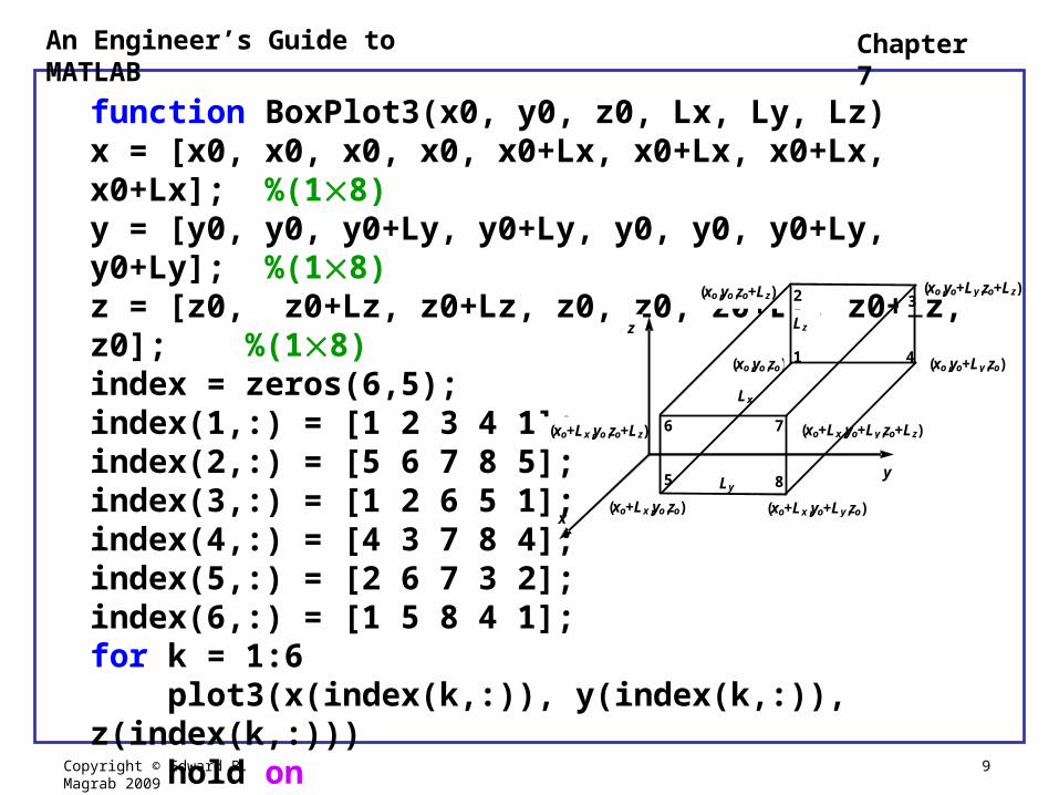
The location and orientation of the box are determined by the coordinates of its two diagonally opposed corners: P(xo,yo,zo) and P(xo+Lx, yo+Ly, zo+Lz).

The script is


Chapter 7

9


function BoxPlot3(x0, y0, z0, Lx, Ly, Lz)x = [x0, x0, x0, x0, x0+Lx, x0+Lx, x0+Lx, x0+Lx]; %(18)y = [y0, y0, y0+Ly, y0+Ly, y0, y0, y0+Ly, y0+Ly]; %(18)z = [z0, z0+Lz, z0+Lz, z0, z0, z0+Lz, z0+Lz, z0]; %(18)index = zeros(6,5);index(1,:) = [1 2 3 4 1];index(2,:) = [5 6 7 8 5];index(3,:) = [1 2 6 5 1];index(4,:) = [4 3 7 8 4];index(5,:) = [2 6 7 3 2];index(6,:) = [1 5 8 4 1];for k = 1:6 plot3(x(index(k,:)), y(index(k,:)), z(index(k,:))) hold onend

(xo,yo,zo)

(xo,yo,zo+Lz)

(xo+Lx,yo,zo)

(xo+Lx,yo,zo+Lz)

(xo+Lx,yo+Ly,zo)

Ly

Lx

Lz

5

6 7

8

1

2 3

4

z

y

(xo,yo+Ly,zo)

(xo,yo+Ly,zo+Lz)

(xo+Lx,yo+Ly,zo+Lz)

x

y

z


Chapter 7

10


We now use BoxPLot3 to generate three boxes with the following dimensions and the coordinates (xo, yo, zo).

Box #1

Size: 357Location: (1, 1, 1)

Box #2

Size: 451Location: (3, 4, 5)

Box #3

Size: 111Location: (4.5, 5.5, 6)


Chapter 7

11


The script to create and display these wire frame boxes is

BoxPlot3(1, 1, 1, 3, 5, 7)BoxPlot3(4, 6, 8, 4, 5, 1)BoxPlot3(8, 11, 9, 1, 1, 1)

function BoxPlot3(x0, y0, z0, Lx, Ly, Lz)

Box #1 Size: 357 Location: (1,1,1)

Box #2 Size: 451 Location: (3,4,5)

Box #3 Size: 111 Location: (4.5,5.5,6)


Chapter 7

12


Example – Sine Wave Drawn on the Surface of a Cylinder

The coordinates of a sine wave on the surface of a cylinder are obtained from the following relations.

cos( )

sin( )

cos( )

x = b t

y = b t

z = c at

If we assume that a = 10.0, b = 1.0, c = 0.3, and 0 t 2, then the script is


Chapter 7

13


t = linspace(0, 2*pi, 200); a = 10; b = 1.0; c = 0.3;x = b*cos(t);y = b*sin(t);z = c*cos(a*t);plot3(x, y, z, 'k')axis equal

cos( )

sin( )

cos( )

x = b t

y = b t

z = c at


Chapter 7

14


Surfaces

A set of 3D plotting functions is available to create surfaces, contours, and variations and specialization of these basic forms.

A surface is defined by the expression

( )z = f x, y

where x and y are the coordinates in the xy-plane and z is the resulting height.


Chapter 7

15


The basic surface plotting functions are

surf(x, y, z)

and

mesh(x, y, z)

where the x, y, and z are the coordinates of the points on the surface.

surf – draws a surface composed of colored patches.

The colors of the patches are determined by the magnitude of z.

mesh – draws white surface patches that are defined bytheir boundary.

The colors of the lines are determined by the magnitude of z.


Chapter 7

16


Example –

Consider the surface created by

4 2 2 2( ) = + 3 + - 2 - 2 - 2 + 6z x, y x x y x y x y

over the range 3 < x < 3 and 3 < y < 13.

We shall place the generation of the x, y, and z coordinate values in an M file so that we can use it in several examples.

We call this function SurfExample.


Chapter 7

17


function [x, y, z] = SurfExamplex1 = linspace(-3, 3, 15); % (115)y1 = linspace(-3, 13, 17); % (117)[x, y] = meshgrid(x1, y1); % (1715)z = x.^4+3*x.^22*x+6-2*y.*x.^2+y.^2-2*y; % (1715)

4 2 2 2( ) = + 3 + - 2 - 2 - 2 + 6z x, y x x y x y x y


Chapter 7

18


Difference Between surf and mesh

[x,y,z] = SurfExample;surf(x, y, z)

[x,y,z] = SurfExample;mesh(x, y, z)

-4-2

02

4

-5

0

5

10

150

50

100

150

200


Chapter 7

19


[x,y,z] = SurfExample;mesh(x, y, z) hidden off


Chapter 7

20


Combining Surfaces and Lines

One can combine 3D plotting functions to draw multiple surfaces and multiple lines.

To illustrate this, we create two functions –

Corners

Draws four lines connecting the corners of the surface generated by SurfExample to the xy-plane passing through z = 0.

Disc

Creates a circular disc that intersects the surface created by SurfExample at zo = 80, has a radius of 10 units, and has its center at (0,5).


Chapter 7

21


The two functions are

function Cornersxc = [-3, -3, 3, 3];yc = [-3, 13, 13, -3];zc = xc.^4+3*xc.^22*xc+62*yc.*xc.^2+yc.^22*yc;hold onplot3([xc; xc], [yc; yc], [zeros(1,4); zc], 'k')

-3-2

-10

12

3

-5

0

5

10

150

50

100

150

200

(3, 3, z(3,3))

(3, 13, z(3,13))

(3, 13, z(3,13))(3, 3, z(3,3))The coordinates of the corners are:


Chapter 7

22


function Disc(R, zo)r = linspace(0, R, 12); % (112)theta = linspace(0, 2*pi, 50); % (150)x = cos(theta')*r; % (5012)y = 5 + sin(theta')*r; % (5012)hold onz = repmat(zo, size(x)); % (5012)surf(x, y, z)

-10

-5

0

5

10

-5

0

5

10

15

79

79.5

80

80.5

81


Chapter 7

23


The script is

[x, y, z] = SurfExample;surf(x, y, z);Disc(10, 80)Corners

-10-5

05

10

-50

510

150

50

100

150

200


Chapter 7

24


Altering Graph Appearance

Several functions that can be used in various combinations to alter the appearance of the resulting surface plot are -

box on or box offgrid on or grid offaxis on or axis off

The function box on only draws a box if axis on has been selected.


Chapter 7

25


Illustration of box, grid, and axis

[x,y,z] = SurfExamplemesh(x, y, z)grid off

[x,y,z] = SurfExamplemesh(x, y, z)axis off grid off

-10-5

05

10

-50

510

150

50

100

150

200


Chapter 7

26


[x,y,z] = SurfExamplemesh(x, y, z)axis on grid offbox on

-10-5

05

10

-50

510

150

50

100

150

200


Chapter 7

27


The colors of either the patches created by surf or the lines created by mesh can be changed to a uniform color using

colormap(c)

where c is a three-element vector, each of whose value varies between 0 and 1.

The first element corresponds to the intensity of red, the second to the intensity of green, and the third to the intensity of blue.


Chapter 7

28


Some Values of the Color Vector Used in colormap(c)

c Color

[0 0 0] [1 1 1] [1 0 0] [0 1 0] [0 0 1] [1 1 0] [1 0 1] [0 1 1] [0.5 0.5 0.5]

black white red green blue yellow magenta cyan gray


Chapter 7

29


Additional Ways to Visually Enhance a Surface

[x,y,z] = SurfExample;meshz(x, y, z)

[x,y,z] = SurfExample;waterfall(x, y, z)

-3-2

-10

12

3

-5

0

5

10

150

50

100

150

200

-3-2

-10

12

3

-5

0

5

10

150

50

100

150

200


Chapter 7

30


02

46

810

1214

16

-5

0

5

10

150

50

100

150

200

[x,y,z] = SurfExample;ribbon(y, z)

[x,y,z] = SurfExample;surfnorm(x, y, z)

-4-3

-2-1

01

23

4

-5

0

5

10

150

50

100

150

200


Chapter 7

31


Contour Plots

Surfaces can also be transformed into contour plots, which are plots of the curves formed by the intersection of the surface and a plane parallel to the xy-plane at given values of z.

The functions

surfc(x, y, z)meshc(x, y, z)

create surfaces with contours projected beneath the surface.

The quantities x, y, and z are the values of the coordinates of points that define the surface.


Chapter 7

32


Illustration of meshc and surfc

[x,y,z] = SurfExample;meshc(x, y, z)grid off

[x,y,z] = SurfExample;surfc(x, y, z)grid off

-3-2

-10

12

3

-5

0

5

10

150

50

100

150

200

-3-2

-10

12

3

-5

0

5

10

150

50

100

150

200


Chapter 7

33


Various contour plots without the surfaces can be created, either with labels or without labels.

The function

contour(x, y, z, v)

creates a 2D contour plot where

x, y, and z are the coordinates of the points that define the surface.

v, if a scalar, is the number of contours to be displayed and, if a vector of values, the contours of the surface at those values of z .

The use of v is optional.


Chapter 7

34


If the contour plot is to be labeled, then we use the following pair of functions.

[C, h] = contour(x, y, z, v)clabel(C, h, v)


Chapter 7

35


Illustration of contour and clabel

[x,y,z] = SurfExample;contour(x, y, z)

[x,y,z] = SurfExample;contour(x, y, z, 4)

-3 -2 -1 0 1 2 3

-2

0

2

4

6

8

10

12

-3 -2 -1 0 1 2 3

-2

0

2

4

6

8

10

12


Chapter 7

36


[x,y,z] = SurfExample;[C, h] = contour(x, y, z);clabel(C, h)

[x,y,z] = SurfExample;v= [10, 30:30:120]; [clabel(C, h, v)

20

20

20

20

20

2020

20

20

40

40

40

40

40

40

40

40

60

60

60

60

60

60

80

80

80

80

80

100

100 100

100120

120 120

120140

140

140160

-3 -2 -1 0 1 2 3

-2

0

2

4

6

8

10

12

10

10

10

10

10

10

30

30 30

30

30

30

30

30

60

60

60

60

60

60

90

90

90

90120

120 120

120

-3 -2 -1 0 1 2 3

-2

0

2

4

6

8

10

12


Chapter 7

37


To display the contours of the surface in 3D, we use

contour3(x, y, z, v)

where

x, y, and z are the coordinates of points that define the surface.

v, if a scalar, is the number of contours to be displayed and, if a vector of values, the contours of the surface at those values of z.

The use of v is optional.

To label the contour plot, we use the pair of functions

[C, h] = contour3(x, y, z, v)clabel(C, h, v)


Chapter 7

38


To fill the region between the 2D contours with different colors, we use

contourf(x, y, z, v)

The values of the colors can be identified using

colorbar(s)

which places a bar of colors and their corresponding numerical values adjacent to the figure.

The quantity s is a string equal to either 'horiz' or 'vert' to indicate the orientation of the bar.

The default value is 'vert'.


Chapter 7

39


Illustration of contour3, contourf, and colorbar

[x,y,z] = SurfExample;[C, h] = contour3(x, y, z);clabel(C, h)

[x,y,z] = SurfExample;[C, h] = contourf(x, y, z);colorbar

-3 -2 -1 0 1 2 3

-2

0

2

4

6

8

10

12

-3-2

-10

12

3

0

5

10

20

40

60

80

100

120

140

160

180

20

20

2020

20

20 20

20

20

40

40

40

40

40

40

40

40

6060

60

60

60

60

80 80

80

80

80

100

100

100

100

120

120

120

120

140

140

140

160

-3 -2 -1 0 1 2 3

-2

0

2

4

6

8

10

12

20

40

60

80

100

120

140

160

180


Chapter 7

40


The properties of the lines and numbering in contour can be altered a similar manner that was done for plot. For example, to have the contour labels created by contour be enlarged to 14 points and for all the contour lines to be blue, we employ the following steps.

[x, y, z] = SurfExample; [C, h] = contour(x, y, z, v)g = clabel(C, h, v);set(g, 'Fontsize', 14)set(h, 'LineColor', ‘b')

10

10

10

10

10

10

30

30 30

30

30

30

30

30

60

60

60

60

60

60

90

90

90

90120

120 120

120

-3 -2 -1 0 1 2 3

-2

0

2

4

6

8

10

12


Chapter 7

41


Generation of Cylindrical, Spherical, and Ellipsoidal Surfaces

One can use a 2D curve as a generator to create surfaces of revolution by using

[x, y, z] = cylinder(r, n)

which returns the x, y, and z coordinates of a cylindrical surface using the vector r to define a profile curve.

The function cylinder treats each element in r as a radius at n equally spaced points around its circumference.

If n is omitted, a value of 20 is used.


Chapter 7

42


Example –

Consider the curve

= 1.1 + sin( ) 0 2r z z π

which is rotated 360 about the z-axis.

Let us take 26 equally spaced increments in the z-direction and 16 equally spaced increments in the circumferential direction.

The script to plot a cylindrical surface is

zz = linspace(0, 2*pi, 26);[x, y, z] = cylinder(1.1+sin(zz), 16);surf(x, y, z)axis off

Axis of rotation


Chapter 7

43


Axis of rotation


Chapter 7

44


To create a sphere, one can use

[x, y, z] = sphere(n);axis equalsurf(x, y, z)

where n is the number of n by n elements that will comprise the sphere of radius 1 centered at the origin.

If n is omitted, then n = 20.

-1

-0.5

0

0.5

1

-1

-0.5

0

0.5

1-1

-0.5

0

0.5

1


Chapter 7

45


To create an ellipsoid, we use

[x, y, z] = ellipsoid(xc, yc, zc, xr, yr, zr, n);axis equalsurf(x, y, z)

which is centered at (xc, yc, zc) and has semi-axis lengths in the x, y, and z directions, respectively, of xr, yr, and zr.

In addition, n is the number of n by n elements that will comprise the ellipsoid.

If n is omitted, then n = 20.

-10

1

-3

-2

-1

0

1

2

3

-1

0

1


Chapter 7

46


Viewing Angle

There are instances when one wants to change the default viewing angle of the 3D image because –

It does not display the features of interest.

Several different views are to be displayed using subplot.

Exploration of the surface from many different views is desired before deciding on the final orientation.

To determine the azimuth and elevation angle of the view, we use

[a, e] = view

where a is the azimuth and e the elevation.


Chapter 7

47


To orient the object, one depresses the Rotate 3D icon in the figure window and orients the object until a satisfactory orientation is obtained.

Upon typing the previous expression in the command window, the values of the azimuth and elevation will be displayed.

These values are recorded and entered in the expression

view(an, en)

to create the desired orientation the next time that the script is executed.

In this expression, an and en are the numerical values of a and e taken from the command window.


Chapter 7

48


Shading

The surfaces created with surf have used the default shading property called 'faceted'.

The function that changes the shading is

shading s

where s is a string equal to

faceted % Default

flat

interp


Chapter 7

49


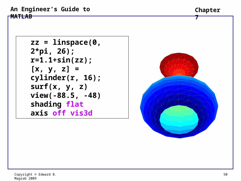
Illustration of view and shading

zz = linspace(0, 2*pi, 26);r=1.1+sin(zz);[x, y, z] = cylinder(r, 16);surf(x, y, z)view(-88.5, -48)shading facetedaxis off vis3d


Chapter 7

50


zz = linspace(0, 2*pi, 26);r=1.1+sin(zz);[x, y, z] = cylinder(r, 16);surf(x, y, z)view(-88.5, -48)shading flataxis off vis3d


Chapter 7

51


zz =linspace(0, 2*pi, 26);r=1.1+sin(zz);[x, y, z] =cylinder(r, 16);surf(x, y, z)view(-88.5, -48)shading interpaxis off vis3d


Chapter 7

52


r = 1+sin(zz);[x, y, z] = cylinder(r, 16);surf(x, y, z)view(-88.5, -48)shading interpcolormap(copper)axis off vis3d


Chapter 7

53


Transparency

The surfaces created with surf can have their opaqueness altered using set and assigning a numerical value to the keyword 'FaceAlpha'.

The effect of this keyword on the resulting surface is dependent on the type of shading chosen.

To illustrate the use of this transparency option, we create a function that generates the numerical values for the surface given by

cos (1 cos )

sin (1 cos )

(1 sin )

v

v

v

x a v u

y a v u

z ba u


Chapter 7

54


If we assume that a = 1.13 and b = 1.14, then the function M file for this surface is

function [x, y, z] = Transparencya = 1.13; b = 1.14;uu = linspace(0, 2*pi, 30);vv = linspace(-15, 6, 45);[u, v] = meshgrid(uu, vv);x = a.^v.*cos(v).*(1+cos(u));y = -a.^v.*sin(v).*(1+cos(u));z = -b*a.^v.*(1+sin(u));


Chapter 7

55


[x, y, z] = Transparency; surf(x, y, z)shading interpaxis vis3d off equalview([-35 38])

[x, y, z] = Transparency; h = surf(x, y, z)set(h, 'FaceAlpha', 0.4)shading interpaxis vis3d off equalview([-35 38])


Chapter 7

56


[x, y, z] = Transparency; h = surf(x, y, z)set(h, 'FaceAlpha', 0.4)axis vis3d off equalview([-35 38])

Note: shading omitted.


Chapter 7

57


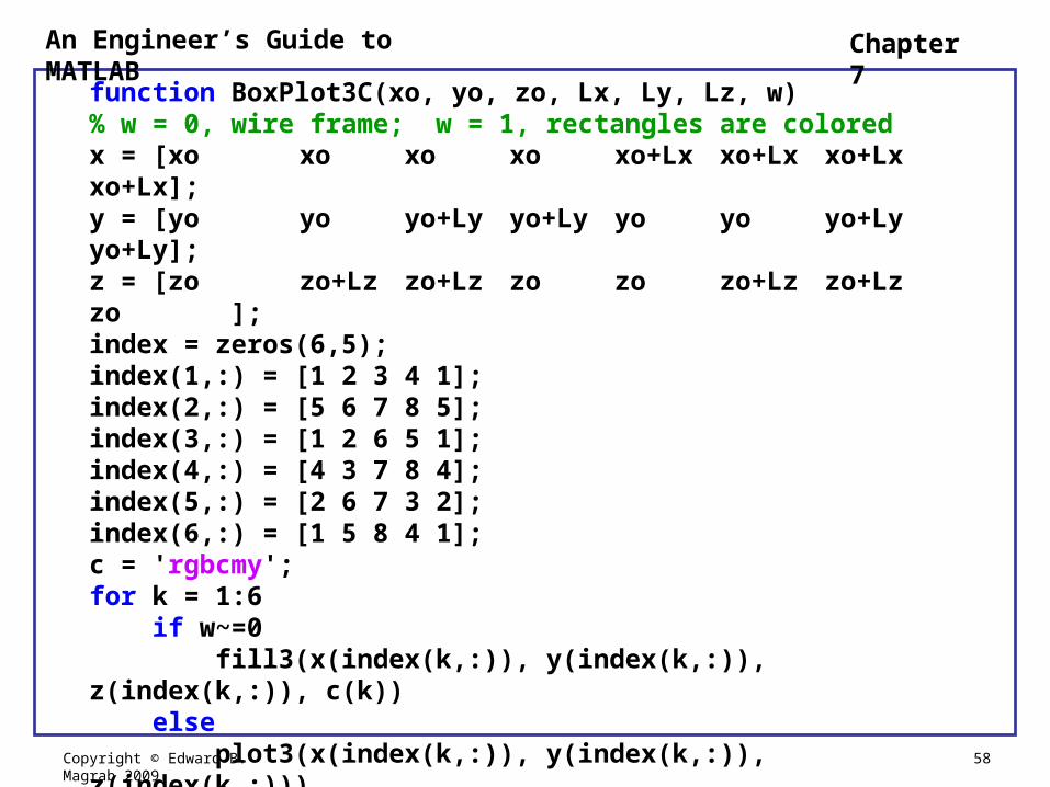
Example - Drawing Wire Frame Boxes: Coloring the Box Surfaces

We modify the M file BoxPlot3 so that all of the six surfaces represented by the rectangles are each filled with a different color.

This modification entails using fill3.

The revised BoxPlot3 is renamed BoxPlot3C and becomes


Chapter 7

58


function BoxPlot3C(xo, yo, zo, Lx, Ly, Lz, w)% w = 0, wire frame; w = 1, rectangles are coloredx = [xo xo xo xo xo+Lx xo+Lx xo+Lx xo+Lx];y = [yo yo yo+Ly yo+Ly yo yo yo+Ly yo+Ly];z = [zo zo+Lz zo+Lz zo zo zo+Lz zo+Lz zo ];index = zeros(6,5);index(1,:) = [1 2 3 4 1];index(2,:) = [5 6 7 8 5];index(3,:) = [1 2 6 5 1];index(4,:) = [4 3 7 8 4];index(5,:) = [2 6 7 3 2];index(6,:) = [1 5 8 4 1];c = 'rgbcmy';for k = 1:6 if w~=0 fill3(x(index(k,:)), y(index(k,:)), z(index(k,:)), c(k)) else plot3(x(index(k,:)), y(index(k,:)), z(index(k,:))) end hold onend


Chapter 7

59


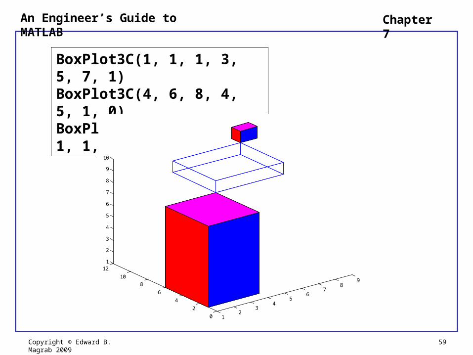
BoxPlot3C(1, 1, 1, 3, 5, 7, 1)BoxPlot3C(4, 6, 8, 4, 5, 1, 0)BoxPlot3C(8, 11, 9, 1, 1, 1, 1)

12

34

56

78

9

0

2

4

6

8

10

121

2

3

4

5

6

7

8

9

10


Chapter 7

60


Example - Intersection of a Cylinder and a Sphere and the Highlighting of Their Intersection

The curve that results from the intersection of a sphere of radius 2a centered at the origin and a circular cylinder of radius a centered at (a, 0) is given by the parametric equations

(1 cos )

sin

2 sin( / 2)

x a

y a

z a

where 0 4.


Chapter 7

61


To create a sphere of radius 2a, we multiply each of the coordinates from the output of sphere by 2a.

The coordinates that are output from cylinder must be altered as follows:

x ax + ay ayz 4az 2a

We assume that a = 1. The script is


Chapter 7

62


a = 1;[xs, ys, zs] = sphere(30);surf(2*a*xs, 2*a*ys, 2*a*zs)hold on[x, y, z] = cylinder;surf(a*x+a, a*y, 4*a*z-2*a)shading interpt = linspace(0, 4*pi, 100);x = a*(1+cos(t));y = a*sin(t);z = 2*a*sin(t/2);plot3(x, y, z, 'y-', 'Linewidth', 2.5);axis equal offview([45, 30])


Chapter 7

63


Example - Enhancing 2D Graphs with 3D Objects: Volume of Sphere and Ellipsoid

For a sphere of radius a and an ellipsoid with its major axis in the x-direction equal to 2a, minor axis in the y-direction equal to 2b, and minor axis in the z-direction equal to 2c, the ratio of the volume of an ellipsoid to the volume of a sphere is

ellipse

sphere

V b cV

V a a

We create the following program to enhance the understanding of a plot of V as a function b/a for several values of c/a.


Chapter 7

64


b = [0.5, 1]; c = b;for k = 1:2 plot(b, b*c(k), 'k-') text(0.75, (b(1)*c(k)+b(2)*c(k))/2-0.02, ['c/a = ' num2str(c(k))]) hold onendxlabel('b/a') ylabel('V')for k = 1:4 switch k case 1 axes('position', [0.12, 0.2, 0.2, 0.2]) [xs, ys, zs] = ellipsoid(0, 0, 0, 1, b(1), c(1), 20); mesh(xs, ys, zs) text(0, 0, 1, ['b/a = ' num2str(b(1)) ' c/a = ' num2str(c(1))]) case 2 axes ('position', [0.1, 0.5, 0.2, 0.2]) [xs, ys, zs] = ellipsoid(0, 0, 0, 1, b(1), c(2), 20); mesh (xs, ys, zs) text (0, 0, 1.5, ['b/a = ' num2str(b(1)) ' c/a = ' num2str(c(2))])


Chapter 7

65


case 3 axes ('position', [0.7, 0.65, 0.2, 0.2]) [xs, ys, zs] = ellipsoid(0, 0, 0, 1, b(2), c(2), 20); mesh (xs, ys, zs) text (-1.5, 0, 2, ['b/a = ' num2str(b(2)) ' c/a = ' num2str(c(2))]) case 4 axes ('position', [0.7, 0.38, 0.2, 0.2]) [xs, ys, zs] = ellipsoid(0, 0, 0, 1, b(2), c(1), 20); mesh (xs, ys, zs) text (-1.5, 0, 1.5, ['b/a = ' num2str(b(2)) ' c/a = ' num2str(c(1))]) end colormap([0 0 0]) axis equal offend


Chapter 7

66


0.5 0.6 0.7 0.8 0.9 10.2

0.3

0.4

0.5

0.6

0.7

0.8

0.9

1

c/a = 0.5

c/a = 1

b/a

V

b/a = 0.5 c/a = 0.5

b/a = 0.5 c/a = 1

b/a = 1 c/a = 1

b/a = 1 c/a = 0.5


Chapter 7

67


Example – Natural Frequencies of a Beam Restrained by a Spring

The natural frequency coefficient for an Euler-Bernoulli hinged at both ends and restrained at an interior point 1 by a spring with nondimensional stiffness Ks is determined from

31 1 2 1( ) ( ) 0s n n n n nK C T C R

1 11 2 2

1 12 2 2

( ) ( [1 ]) ( ) ( [1 ])

( ) ( )

( ) ( [1 ]) ( ) ( [1 ])

( ) ( )

( ) 0.5 sinh sin

( ) 0.5 sinh sin

n n n nn

n n

n n n nn

n n

T T R RC

R T

T R R TC

R T

R x x x

T x x x

where


Chapter 7

68


There are two parameters that are of interest: 1 and

Ks.

We shall generate a surface of the lowest natural frequency coefficient 1 as a function of 1 and

log10(Ks).

Then we shall use these same natural frequency coefficients to create a contour plot of log10(Ks) versus

1 for several values of 1/.

The program is


Chapter 7

69


function BeamWithSpringNeta1 = 28; NKs = 21; Kend = 4;Ks = logspace(0, Kend, NKs);Om = linspace(0.02, 10, 50);Omeg = zeros(Neta1, NKs);eta1 = linspace(0, 1, Neta1); for et = 1:Neta1 for kss = 1:NKs D = NFEqnBeamWithKs(Om, Ks(kss), eta1(et)); for k = 2:length(Om) if D(k)*D(k-1) < 0 Omeg(et, kss) = fzero(@NFEqnBeamWithKs, …

[Om(k-1), Om(k)], [], Ks(kss), eta1(et)); break end end endend


Chapter 7

70


figure(1)mesh(eta1, log10(Ks), (Omeg/pi)')xlabel('\eta_1')ylabel('log_{10}(K_s)')zlabel('\Omega_1/\pi')view([-15,30])a = axis; a(4) = Kend;axis(a)figure(2)[C, h] = contour(eta1, log10(Ks), (Omeg/pi)');clabel(C, h)xlabel('\eta_1')ylabel('log_{10}(K_s)')


Chapter 7

71


function C = NFEqnBeamWithKs(Om, Ks, eta1)CA = T(Om*eta1).*(T(Om).*T(Om*(1-eta1))-R(Om).*R(Om*(1-eta1)));CB = R(Om*eta1).*(T(Om).*R(Om*(1-eta1))-R(Om).*T(Om*(1-eta1)));C = CA+CB+(R(Om).^2-T(Om).^2)*Om.^3/Ks;

function r = R(x)r = 0.5*(sinh(x)+sin(x));

function t = T(x)t = 0.5*(sinh(x)-sin(x));


Chapter 7

72



Chapter 7

73



Chapter 7

74


Example – Rotation and Translation of 3D Objects: Euler Angles

The rotation and translation of a point p(x,y,z) to another location P(X,Y,Z) is given by

11 12 13

21 22 23

21 22 23

x

y

z

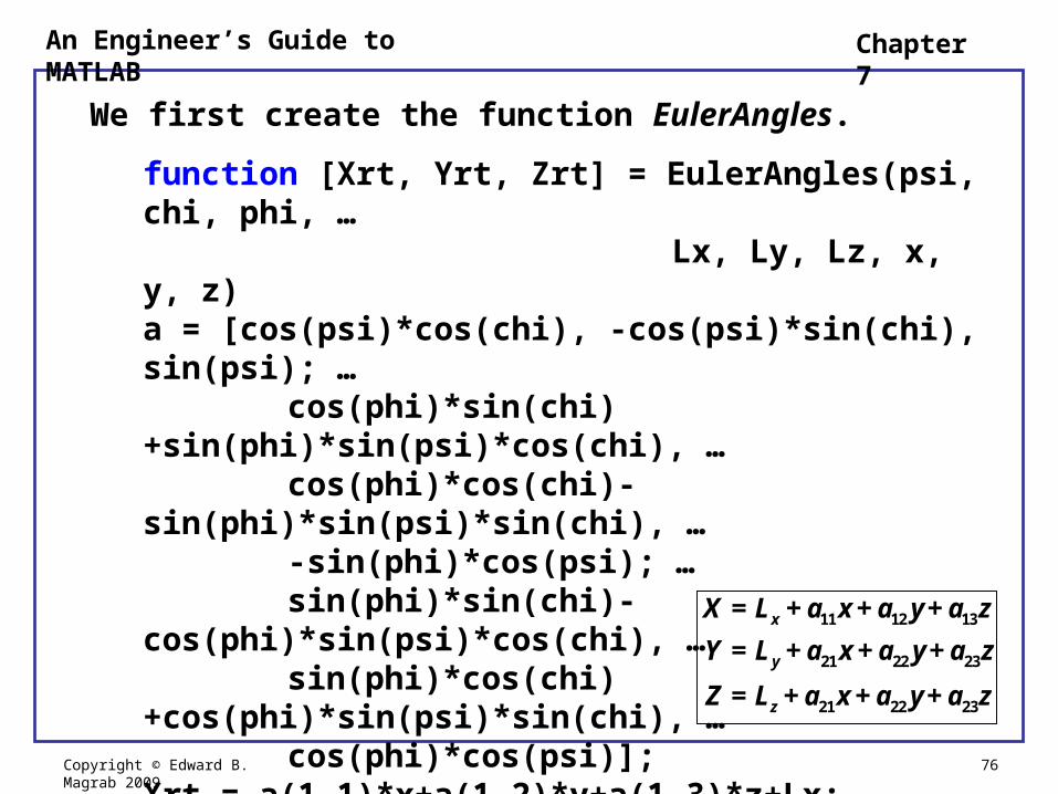
X = L + a x + a y + a z

Y = L + a x + a y + a z

Z = L + a x + a y + a z

where Lx, Ly, and Lz are the x, y, and z components of the translation, respectively, and aij, i, j = 1, 2, 3, are the elements of

cos cos -cos sin sin

= cos sin + sin sin cos cos cos - sin sinψsin -sin cos

sin sin - cos sin cos sin cos + cos sinψsin cos cos

ψ χ ψ χ ψ

a φ χ φ ψ χ φ χ φ χ φ ψ

φ χ φ ψ χ φ χ φ χ φ ψ


Chapter 7

75


The quantities , , and are the ordered rotation angles (Euler angles) of the coordinate system about the origin –

about the x-axis

then about the y-axis

then about the z-axis

In general, (x,y,z) can be scalars, vectors of the same length, or matrices of the same order.


Chapter 7

76


We first create the function EulerAngles.

function [Xrt, Yrt, Zrt] = EulerAngles(psi, chi, phi, … Lx, Ly, Lz, x, y, z)

a = [cos(psi)*cos(chi), -cos(psi)*sin(chi), sin(psi); … cos(phi)*sin(chi)+sin(phi)*sin(psi)*cos(chi),

… cos(phi)*cos(chi)-sin(phi)*sin(psi)*sin(chi),

… -sin(phi)*cos(psi); … sin(phi)*sin(chi)-cos(phi)*sin(psi)*cos(chi),

… sin(phi)*cos(chi)+cos(phi)*sin(psi)*sin(chi),

… cos(phi)*cos(psi)];

Xrt = a(1,1)*x+a(1,2)*y+a(1,3)*z+Lx;Yrt = a(2,1)*x+a(2,2)*y+a(2,3)*z+Ly;Zrt = a(3,1)*x+a(3,2)*y+a(3,3)*z+Lz;

11 12 13

21 22 23

21 22 23

x

y

z

X = L + a x + a y + a z

Y = L + a x + a y + a z

Z = L + a x + a y + a z


Chapter 7

77


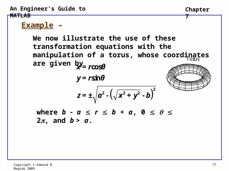
Example –

We now illustrate the use of these transformation equations with the manipulation of a torus, whose coordinates are given by

22 2 2

cos

sin

x = r θ

y = r θ

z = ± a - x + y - b

where b a r b + a, 0 2, and b > a.

Torus = 60

= 60 = 60 = 60


Chapter 7

78


We first create the following function to obtain the coordinates of the torus.

function [X, Y, Z] = Torus(a, b)r = linspace(b-a, b+a, 10); th = linspace(0, 2*pi, 22);x = r'*cos(th); y = r'*sin(th); z = real(sqrt(a^2-(sqrt(x.^2+y.^2)-b).^2));X = [x x]; Y = [y y]; Z = [z -z];

where real is used to eliminate any small imaginary parts caused by numerical round-off.

22 2 2

cos

sin

x = r θ

y = r θ

z = ± a - x + y - b

Torus = 60

= 60 = 60 = 60


Chapter 7

79


We obtain four plots of the torus:

(1) No rotations.

(2) Rotated 60 about the x-axis ( = 60) and compared to the orientation of the original torus.

(3) Rotated 60 about the y-axis ( = 60) and compared to the orientation of the original torus.

(4) Rotated 60about the x-axis ( = 60), rotated 60 about the y-axis ( = 60) and compared to the orientation of the original torus.

We assume that a = 0.2 and b = 0.8 and we use colormap to produce a mesh of black lines.


Chapter 7

80


The script is[X, Y, Z] = Torus(0.2, 0.8);psi = [0, pi/3, pi/3]; chi = [0, 0, 0]; phi = [pi/3,0, pi/3];Lx = 0; Ly = 0; Lz = 0;for k = 1:4 subplot(2,2,k)

if k==1 mesh(X, Y, Z) else mesh(X, Y, Z) hold on [Xr Yr Zr] = EulerAngles(psi(k-1), chi(k-1), … phi(k-1), Lx, Ly, Lz, X, Y, Z); mesh(Xr, Yr, Zr) end


Chapter 7

81


switch k case 1

text(0.5, -0.5, 1, 'Torus') case 2

text(0.5, -0.5, 1,'\phi = 60\circ') case 3 text(0.5,-0.5,1,'\psi = 60\circ') case 4

text(0.5, -0.5, 1.35,'\psi = 60\circ')text(0.55, -0.5, 1,'\phi = 60\circ')

end colormap([0 0 0]) axis equal off grid offend


Chapter 7

82


Torus = 60

= 60 = 60

= 60

an engineer’s guide to matlab 3rd edition chapter 7 3d graphics

Documents