an empirical study of regional convergence, inequality
TRANSCRIPT
An empirical study of regional convergence, inequality, and
spatial dependence in the enlarged European Union
John Källström
August, 2012
NEKN01, Master Thesis I
Department of Economics, Lund University
Supervisor: Joakim Gullstrand

1
Abstract
This thesis deals with regional convergence and the spatial dynamics of regional incomes in the
enlarged EU. The aim is to build on prior work in the field, to investigate convergence dynamics
of regions in the newest EU member states and to look at the importance of country and spatial
effects in the convergence process. Examining per-capita income growth among 1309 NUTS 3-
regions across the EU over 1995-2009, very slow rates of both β- and σ-convergence is found.
Spatial data analysis reveals strong spatial dependence and clustering of regional incomes and
growth rates across EU regions. By spatial econometric methods it is found that the spatial
dependence in the convergence process is mainly contained to regions within the same country.
Thus, regional growth spillovers seem to a large extent stop at country borders. Moreover,
convergence in the old member states over the sample period is found to be mainly due to
growth among low-income regions. Conversely, no significant convergence can be found among
the newest member states. Rather these countries show evidence for increasing income
inequality. This is found to be mainly attributed to increasing within-country regional income
disparities.
Keywords: regional income inequality, β-convergence, σ-convergence, spatial econometrics,
exploratory spatial data analysis, spatial dependence, European Union.
2
Table of contents
1. Introduction ............................................................................................................................................................. 4
2. Theoretical foundation ...................................................................................................................................... 6
2.1. Neoclassical theory and regional convergence ............................................................................... 6
2.1.1. Neoclassical convergence hypotheses ...................................................................................... 7
2.1.2. Spatial dependence in the neoclassical setting .................................................................... 7
2.2. Endogenous growth and new economic geography ..................................................................... 9
2.2.1. New economic geography ............................................................................................................ 9
2.2.2. Agglomeration and regional growth .................................................................................... 10
3. Methodological aspects ................................................................................................................................... 12
3.1. β-convergence ........................................................................................................................................... 12
3.2. Spatial dependence.................................................................................................................................. 13
3.2.1. Nuisance spatial dependence ................................................................................................... 14
3.2.2. Substantive spatial dependence .............................................................................................. 15
4. Prior research ...................................................................................................................................................... 16
4.1. The regression approach ...................................................................................................................... 17
4.1.1. Spatial dependence and regional convergence ................................................................. 17
4.2. The distributional approach ................................................................................................................ 19
5. Data ............................................................................................................................................................................ 21
6. Analysis .................................................................................................................................................................... 24
6.1. The regional income distribution ...................................................................................................... 24
6.1.1. Inequality patterns ...................................................................................................................... 25
6.1.2. Transition dynamics .................................................................................................................... 30
6.1.3. Polarization patterns .................................................................................................................. 32
6.2. Exploratory spatial data analysis ...................................................................................................... 36
6.2.1. Global spatial autocorrelation ................................................................................................ 36
6.2.2. Local spatial autocorrelation .................................................................................................. 38
6.3. Regression results .................................................................................................................................... 42
3
6.3.1. OLS-estimations ............................................................................................................................ 43
6.3.2. Spatial econometric estimations ............................................................................................ 45
7. Conclusions ............................................................................................................................................................ 47
References ................................................................................................................................................................... 52
Appendix I .................................................................................................................................................................... 55
Appendix II .................................................................................................................................................................. 56
Appendix III ................................................................................................................................................................ 57
Appendix IV................................................................................................................................................................. 58
List of figures
6.1. Entropy indices, EU28………………………………………………………………………………………………..26
6.2. Share of between- and within-country component of regional inequality, EU28…………...27
6.3. Entropy indices, EU15………………………………………………………………………………………………..28
6.4. Share of between- and within-country component of regional inequality, EU15…………...28
6.5. Entropy indices, NMS…………………………………………………………………………………………………29
6.6. Share of between- and within-country components of regional inequality, NMS…………...29
6.7. Density function for EU28 relative per-capita GRP 1995 and 2009……………………………….34
6.8 Density function for EU15 relative per-capita GRP 1995 and 2009………………………………..34
6.9. Density function for NMS relative per-capita GRP 1995 and 2008………………………………..35
6.10. Moran scatterplot per-capita GRP 1995, EU28…………………………………………………………..39
6.11. Moran scatterplot growth rates 1995-2009, EU28…………………………………………………….40
6.12. Local spatial autocorrelation per-capita GRP 1995, EU28………………………………………….41
6.13. Local spatial autocorrelations growth rates 1995-2009, EU28…………………………………..42
List of tables
6.1. Transition table of relative per-capita GRP 1995-2009, EU28………………………………………30
6.2. Transition table of relative per-capita GRP 1995-2009, EU15………………………………………30
6.3. Transition table of relative per-capita GRP 1995-2009, NMS………………………………………..31
6.4. Moran’s I-test of global spatial autocorrelation, EU28………………………………………………….37
6.5. OLS estimation, 1995-2009....……………………………………………………………………………………..43
6.6. SEM estimation, 1995-2009.……………………………………………………………………………………….46
6.7. SLM estimation, 1995-2009.……………………………………………………………………………………….46
4
1. Introduction
The entry of ten new member states1, many from the former Soviet bloc, into the EU in 2004
meant that income disparities doubled in the union. The average per-capita incomes of the new
member states (NMS) amounted to about 50% of the old members (Niebuhr and Schlitte 2004).
In 2007 two additional former Eastern bloc countries – Romania and Bulgaria – with a below
average incomes joined the union. Thus, between-country inequalities in the enlarged EU are
large. However, income disparities are even larger within countries than between. For example,
in 2009 West Inner-City London, in the United Kingdoms, had a per-capita gross regional
product (GRP) of 140 100 measured in Purchasing Power Standard (PPS). This amounts the
highest per-capita income in the union, about six times the EU average. At the same time, the
region of Vaslui in Romania had a GRP per capita of 5500 PPS, about one fourth of the EU
average. Thus, regional inequalities within EU-countries are even more pronounced than
between. However, if the disparities are growing or if poorer regions are catching up,
converging, to the richer ones is a more debatable issue.
Many theoretical and empirical contributions stress the importance of economic integration in
reducing economic inequality. For example, neoclassical theory predicts that intensified
economic integration will lead to poorer regions converging to richer ones. In this view,
decreased trade barriers facilitate the equalization of factor returns and proportions and
technological diffusion, which in turn contributes to capital deepening and technological growth
and thus to per-capita income growth. On the other hand, insights from endogenous growth
models and new economic geography show that regional convergence need not be a definite
outcome of economic integration and that geographical location matter for economic outcome.
Instead these views stress that integration allows economic activity to cluster by agglomerative
and cumulative processes driven by externalities with a strong spatial dimension. As a result, the
geographical distribution of economic activity is spatially dependent and persistent: regions
with low (high) incomes are surrounded by other regions with low (high) incomes and tend to
remain so over time.
Following Ertur et al. (2006), a couple of stylized facts on regional convergence in Europe can be
drawn from the empirical literature. First, the convergence rate seems to be very slow among
European regions. Second, regional income disparities seem persistent despite the ongoing
integration process. To this can be added that the regional income disparities in Europe show a
distinct and persistent geographical core-periphery pattern (see e.g. Bräuninger and Niebuhr
1 Cyprus, Estonia, Latvia, Lithuania, Malta, Poland, Slovakia and Slovenia
5
2005; Fischer and Stirböck 2006; Battisti and Di Vaio 2008). That is to say, poor and regions are
clustered in space with other poor regions and rich with other rich regions.
Investigating convergence and spatial interaction between regions is of great importance if the
European integration process is to be fully understood. Are poorer regions catching-up to richer
ones and how is the ongoing European integration process affecting this? Are incomes in the
NMS catching up to the old pre-2004 members (EU15)? In light of the suggested importance of
geography, how important is regional neighborhood compared to country for determining the
convergence process of EU regions? That is, do spatial dependence matter more for a regions’
growth performance than country effects? All these questions have large policy implications.
Particularly as one of the stated goals of the EU, stated in both the Maastricht-treaty and Single
Market act, is increased regional income cohesion. However, how well the EU work to foster this
process is debatable. This thesis hopes to bring some clarity and new insights to this area.
Early studies of regional convergence failed to explicitly account for spatial dependence, instead
treating each region as separate units. However, recent developments in spatial econometrics
allow regional spatial interactions to be accounted for. Moreover, critique against conventional
convergence analysis based on cross-section regressions stress that to fully appreciate if
convergence is accompanied with lessened inequality the dynamics of the entire income
distribution must be taken into account (see e.g. Quah 1993a, 1993b). In light of these results,
this thesis will investigate the link between agglomeration, spatial spillovers, and growth in the
context of European regions taking both a parametric spatial econometric approach and a
nonparametric distributional approach. Most previous studies focus on either the one or the
other approach. But this thesis argues that to get the full picture of regional income convergence
both traditional regression analyses and distributional analysis should be accounted for.
The thesis has three aims. First, it builds and extends on the prior work in the field of regional
income convergence and spatial dependence. This is done by employing a comparably larger
cross-section of European regions over the period 1995-2009. In addition, the regional data is at
a lower geographical aggregation level than what has commonly been used in previous studies.
Following the discussion above, complementary to the traditional regression analysis a
distributional analysis of regional incomes will also be performed. Second, the thesis aims at
identifying differences in the convergence dynamics among regions in the new and old member
states. This is done to investigate if the NMS are converging to the EU-average. This can be
viewed as an implicit way to investigate if joining the EU facilitates convergence among poorer
regions. Third, the aim is to tentatively appraise if spatial dependence in the convergence
processes in the EU mainly is a national or neighborhood phenomenon. Previously, Paas and
Schlitte (2007, 2008) and Bräuningen and Niebuhr (2005) among others have shown the

6
importance of country-specific effects in the regional convergence process of Europe, a similar
analysis will be carried out here.
If spatial dependence and clustering is found to mainly be an outcome determined by
neighborhood this could be viewed as implicit evidence that agglomeration economies brought
on by the European integration process is more important than national characteristics in
creating clusters of economic activity. Thus, the thesis could be viewed as an evaluation of the
extent of “integration forces” and their effect on regional income convergence in the EU. As
mentioned above, increased regional cohesion is one of the main pillars of the European
integration so evaluating this process has important policy implications. Moreover, since the
eastward expansion of the EU, income disparities within the union have increased markedly.
Hence, to evaluate if incomes in the NMS are growing should be of outmost importance.
The disposition of the thesis is as follows. In chapter 2 the theoretical foundations underlying
the notion of regional convergence and spatial dependence are stated. Following this in chapter
3 some methodological aspects of the convergence analysis and spatial dependence are covered.
In chapter 4 a description of the current state of research is given. Next, in chapter 5, the
employed dataset is discussed. Then, in chapter 6, the empirical analysis of the thesis is given.
First, a distributional analysis is preformed to account to for regional income disparities. Second,
the data is described by means of spatial data analysis. Third, the rate of regional convergence
and the importance of spatial- and country-effects is estimated by means of a spatial
econometric analysis. Lastly, in chapter 7, the main findings are summarized and some
concluding remarks, policy implications and suggestions for future research are given.
2. Theoretical foundation
The theoretical predictions on the effects of economic integration on regional income
convergence are varied. The neoclassical theory predict that as trade barriers between countries
and regions fall the returns to factors equalize, which will lead to income convergence and
decreasing disparities. On the other hand, in the so called endogenous growth models and in
new economic geography (NEG), integration need not bring about convergence. Instead, it can
result in increased regional income disparities and divergent growth trends.
2.1. Neoclassical theory and regional convergence
Neoclassical growth provides a rationale for economic integration resulting in regional per-
capita income convergence. Following Magrini (2004) and Aghion and Howitt (2004), in this set
of models, growth is determined by the marginal productivity of production factors, e.g. capital
or labor, and the exogenous given technological growth rate.
7
2.1.1. Neoclassical convergence hypotheses
In neoclassic models, economic integration fosters trade and factor mobility, which in turn
fosters income convergence. The prediction of convergence in the neoclassical setting comes
from the assumption of diminishing returns to production factors. This implies that economies
with a relative scarce endowment of a specific factor will have a higher marginal return to this
factor. Typically it is assumed that economies with a relatively low capital-labor ratio will have a
lower per-capita output, but higher growth rate, as a lower capital stock means higher marginal
productivity and returns to capital (Magrini 2004: p.2745). So, increasing trade or the mobility
of factors leads to faster equalization of both factor proportions and returns. That is to say,
poorer (low capital-labor ratio) economies will grow faster than richer (higher capital-labor
ratio), eventually catching up with these. In the long run all regions will be at the same income-
level and grow at the exogenous given rate of technological progress. This state is referred to as
the steady state of the economy.
The prediction that the only thing separating rich economies from poor is the capital stock and
that poorer economies eventually will catch-up with their richer counterparts when enough
capital has been accumulated is known as the unconditional convergence hypothesis. On the
other hand, convergence in income levels or growth rates conditioned on the underlying
structural characteristics of an economy or differences in production technologies is known as
the conditional convergence hypothesis (Aghion and Howitt 2004: p.56). According to the
conditional convergence hypothesis economies with different factor endowment, preferences
technology, institutions etc. will converge to different steady-states. Moreover, if groups (clubs)
of economies with similar characteristic converge to the same per-capita income-level and
growth rate in the long-run, conditional converge is often referred to as club-convergence. Note
that there need be no convergence between clubs (Martin 2001).
Explanations for regional club-convergence range from the endowment of a wide range of
production factors (e.g. human capital formation, public infrastructure, R&D activity) to local
preferences or government policies (Canova 2004). Moreover, as Bräuninger and Niebuhr
(2004) point out, the club-convergence hypothesis provides an rationale for the influence of
national policies, legislation etc. on the regional convergence-process. Thus from this
perspective, country-specific effects are expected to be a very influential factor in the regional
convergence process.
2.1.2. Spatial dependence in the neoclassical setting
One of the conditions for unconditional income convergence is evenly spread technology. This is
arguably a rather strong assumption. As is argued in this thesis and others, regional incomes
8
appear to be strikingly unevenly distributed and geographical location seems to matters for
economic outcome. López-Bazo et al. (2004), Egger and Pfaffermayr (2006) and Ertur and Koch
(2007) all present examples of neoclassical models that take geographical location into account
and shows how spatial interaction can affect the growth and convergence process. Specifically,
they assume regional interdependence through spatially-bounded externalities in (human or
physical) capital accumulation.
Generally, the implication stemming from accounting for regional interdependence is that
economies need no longer perfectly share technology. In turn this implies that a region’s capital
accumulation now also depends on the capital accumulation of its neighbors. In a neoclassic
setting this gives that economic activity and incomes no longer need to be evenly distributed. As
for example Fischer and Stirböck (2006: pp.694-5) argues, if such interdependence is bounded
geographically they can give rise to convergence clubs conditioned on spatial neighborhoods.
From López-Bazo et al. (2004), Egger and Pfaffermayr (2006) and Ertur and Koch (2007), a few
general conclusions from considering spatial externalities in capital accumulation can be drawn.
First, technological diffusion has a positive effect on the capital intensity of a region. From the
assumption of diminishing returns to capital, the rate of investment in physical and human
capital is still a decreasing function of the internal capital stock, but now an increasing function
of the external capital stock of neighbors. This relationship gives that the investment and
accumulation of physical and human capital will be higher in those regions surrounded by other
regions with relatively large capital stocks. Secondly, the models give that the growth rate still is
inversely related to the internal capital intensity, but that it now also depends on the
productivity and growth rates of neighbors, which can counteract the internal diminishing
returns. This implies that the growth rates of two economies with identical internal
characteristics can still differ if they have different neighbors. Thirdly, the rate of convergence
could either be slowed down or spurred on by growth spillovers from neighboring regions.
Hence, by considering technological interdependence between regions a heterogeneous spatial
distribution of both income levels and growth rates can be explained. Neighborhoods of capital-
intensive regions with high incomes and low growth rates are geographically clustered because
of spatial externalities in capital accumulation. Of course the opposite holds for neighborhoods
of low capital-intensity, low incomes and high growth rates. Note how extending the neoclassical
setting to account for spatial spillovers does not change the basic prediction of neoclassic theory.
That is, capital-scarce economies exhibit higher growth rates than capital-intensive economies
and eventually catch up to these. Instead, the extensions give what could be called a
geographical conditional-convergence hypothesis, where the neighborhood dictates the steady
state and growth path of a region. Neighborhoods of similar regions will then converge to the
9
same steady state. Thus, as argued by López-Bazo et al. (2004: p.44), even and uneven economic
development is possible and depends on the relative strength of returns both internal to the
economy and external spillovers from neighbors.
2.2. Endogenous growth and new economic geography
In the above discussion regions converged because of the diminishing returns to capital.
However, the assumptions of diminishing returns have been questioned, see e.g. the discussion
in Aghion and Howitt (2004: pp.56-60). Instead, if investments in innovation (R&D) are
considered, the return on these investments work against the diminishing returns and the
economy can sustain ever increasing technological growth and increasing returns to factors, as
shown by Romer (1986) and Lucas (1988). These kinds of models, incorporating innovation and
thus endogenizing technological growth, have become known as endogenous growth models
(Aghion and Howitt 2004: p.47). As argued by Coe and Helpman (1995: p.860): “In a world with
international trade in goods and services, foreign direct investment, and an international exchange
of information and dissemination of knowledge, a country’s productivity depends on its own R&D as
well as the R&D of trade partners”. Certainly, if regions are considered more open than countries,
this importance should be even more valid between regions than between countries. Note how
endogenous models need not predict convergence between rich and poor economies as in the
neoclassical theory. Instead, by investing in human capital and R&D, high-income regions can
keep up a higher growth rate indefinitely.
Furthermore, as stressed by NEG, other pecuniary externalities than the typical Marshallian
technological and knowledge spillovers, considered in neoclassical and endogenous models,
might be present. Following the work by Krugman (1991), Krugman and Venables (1995), Puga
and Venables (1996) and Fujita et al. (1999), in this set of NEG-models increasing returns to
scale at the firm-level, factor mobility and trade cost work together to induce agglomerations of
economic activity at the aggregate level.
2.2.1. New economic geography
In NEG-models demand linkages create a causal circularity of centrifugal and centripetal forces
that divide the economy into a high-income core and a low-income periphery. Centrifugal forces
are forces that work toward the geographical dispersion of economic activity. Any costs (both
pecuniary costs and negative externalities) that can be associated with living or running a
business in an economic center – such as housing prices, congestion or local competition – are
centrifugal forces. Centripetal forces, on the other hand, work toward the spatial agglomeration
10
of economic activity through what is sometimes referred to as forwards- and backwards-
linkages.2
First consider the case of forward linkages. Firms wish to locate in regions with good access to
large markets to realize scale economies and minimize transport costs. Consequently, firms will
locate as close to large-market regions, so that they can sell goods to as many as possible and
incur minimal transport costs. Subsequently, they will also attract workers, who in turn will
spend their income locally, further increasing market size (thus demand) and in turn attracting
even more firms wanting to exploit further increasing returns to scale. The backwards linkages,
on the other hand, work through the vertical production chain between firms. In a world of
transport costs, if firms are clustered it is much cheaper to buy inputs, intermediates etc. from
nearby suppliers. Thus, firms will locate near suppliers since the cost of intermediates are lower
there. This tendency for firms to want to shorten input-linkages creates a propensity for firms to
cluster is space.
Hence, if backward- and forward-linkages are strong enough – i.e., if firms can exploit
sufficiently large scale economies; demand is large enough; and, trade costs are adequately low –
the NEG-models gives a demand-linked circular causality that creates what Krugman (1991)
dubbed a core-periphery pattern. That is, following Baldwin and Martin (2004) and letting
capital be the only mobile factor3, firms will cluster together in the region with the initial larger
capital stock, this in turn increases their profits and the return to capital in that region.
Subsequently, as capital flows into the region, the return to capital rises, raising real incomes,
which in turn increases market size and demand further, attracting even more firms. Thus,
capital-intensive industries will agglomerate to the economically larger region, the core, pushing
up incomes, leaving the other region, the periphery, with lower incomes. Hence, history and
endowments determines which region can exploit the demand-circular causality and end up as
the core region, where industry agglomerates.
2.2.2. Agglomeration and regional growth
Bringing the predictions of endogenous growth theory to a NEG-framework, a self-reinforcing
process between growth and agglomeration is commonly found. That is to say, growth brings
about agglomeration and agglomeration brings about growth. However, if these models predict
2 It is also possible to add labor-market pooling to this list. That is, it is much easier for employers to find specialized labor if the labor market is pooled in one location. However, this reason for firms and workers to agglomerate is not included by Krugman (1991). 3 This assumption is made so that the equilibrium will be stable, assuming labor mobility would have created an unstable equilibrium (Baldwin and Martin 2004: pp.2674-5). To avoid a catastrophic outcome where all economic activity agglomerates to one region, NEG models often assumes that one factor is mobile and the other immobile.
11
regional convergence or divergence crucially depend on the assumptions made (Baldwin and
Martin 2004). Generally, the analyses can be divided between models that assume global
technological spillovers and models that assume local technological spillovers (Bräuninger and
Niebuhr 2005: p.3). For instance, following Martin and Ottaviano (1999) and Baldwin and
Martin (2004), when spillovers are of global reach geography do not affect growth. In this
perspective higher growth is associated with convergence since the factors that increase
endogenous growth (R&D-investments, education, etc.) also decrease income disparities.
On the other hand, when spillovers are assumed to be of local character the geographical
concentration of economic activity is found to increase both growth and income disparities. Note
how there is a trade-off between regional income equity and growth, as agglomeration in these
models reduces the cost of innovating in the core but increases the growth rate for the entire
economy. Thus, with localized spillovers an increase in the spatial concentration of economic
activity can be beneficial to growth rates in both the core and the periphery. This means that a
more uneven economic geography is not necessarily bad for the periphery. Nevertheless, note
that for a given geography of production, less localized (i.e. more global) spillovers implies a
lower overall cost of innovation and a higher aggregate growth rate for the entire economy.
Generally the NEG and endogenous growth models underlines the importance of the barriers to
the spatial diffusion of technological and knowledge spillovers. Paraphrasing Baldwin and
Martin (2004), if barriers to the diffusion of technology and innovation are sufficiently low the
periphery can break the vicious demand-linked causality and instead enter a virtuous circle.
That is, start investing, attract industry and thus increase incomes and growth rates. Hence, as
spillovers become less localized the market size of the periphery increases, the cost of
innovating falls and incomes between the core and the periphery will converge.
The endogenous growth and NEG models show that factor mobility and economic spillovers are
important aspects of economic integration. In particular, these can either lessen or extenuate the
centrifugal and centripetal forces implied by freer trade in traditional NEG-models. If spillovers
are localized, the continual lowering of trade costs can produce an uneven spatial development,
as real incomes rises in the core and falls in the periphery. However, now the emergence of
regional imbalances may be accompanied by faster growth in all regions. This creates a tension
between static losses due to income reallocation and dynamic gains due to higher aggregate
growth. Thus from a welfare perspective, while the core is made unambiguously better off by
agglomeration, the welfare effects in the periphery are more ambiguous. Consequently, regional
policies that seek to hinder geographic concentration may cost a country as a whole in terms of
growth.
12
Furthermore, note that there are large differences between core and periphery when it comes to
industrial agglomeration, human capital endowment, R&D activity, and infrastructure etc.
Hence, the NEG and endogenous growth models reinforces and complements the theoretical
predication of geographically conditioned club-convergence from the neoclassical models
discussed above. Instead, the models open up the black box of neoclassical convergence and
describe a certain aspect of how spatial spillovers affect the convergence process.
3. Methodological aspects
Traditionally, empirical tests of the neoclassical convergence hypotheses follow from Baumol
(1986). Baumol implements a simple cross-section regression with the average growth rate as
the dependent variable and initial GDP as the independent variable. Drawing from the
predictions of the neoclassical convergence hypotheses, economies with low initial GDP are
expected to grow faster than economies with higher initial GDP. Thus, a negative estimated
coefficient in Baumol’s specification is interpreted as unconditional convergence. Following
Baumol’s original work, Barro and Sala-i-Martin (1991, 1992) extend the analysis to the
conditional convergence-hypothesis by allowing economies to converge to different steady
states. These approaches of testing unconditional and conditional convergence have by Barro
and Sala-i-Martin been labeled β-convergence regressions.
Moreover, as discussed in chapter 2, spatial dependence is predicted to be an important factor
when regional convergence is considered. Recent developments in spatial econometrics have
been incorporated in the traditional β-convergence analysis. By means of these approaches the
strength and significance of spatial externalities can indirectly be estimated.
3.1. β-convergence
The point of departure of the empirical analysis is the unconditional β-convergence cross-
section of Baumol (1986). Specifically the following model is specified,
(
) , (3.1)
where is per-capita GRP for region i at time t, so that (3.1) gives the relation between initial
per-capita GRP at time t as the independent variable and the average growth rate between time t
and T as the dependent variable. The variable represents the error term. Using OLS-
estimations it is assumed that is identical and independently distributed with zero mean and
constant variance. Moreover, and are parameters to be estimated. The parameter is the
intercept. As discussed in section 2, neoclassical growth theory predicts that the growth rate of

13
an economy is positively related to the distance from its steady state. So, whenever the
independent variable, , shows a negative relationship this is interpreted as β-convergence. In
other words, regions with lower initial per-capita GRP are expected to exhibit relatively higher
average growth rate. The annual rate of β-convergence is obtained from,
.
From this the half-life, i.e. the necessary time for half the differences in per-capita incomes to
disappear, can be obtained from .
However, as noted in section 2 the steady-state can differ across economies, being conditioned
on underlying characteristics specific to each economy. Specifically to this thesis, country-
specific characteristics will be accounted for, so that regions belonging to different countries will
be allowed to converge to different steady states. Thus in addition to the unconditional
convergence model in (3.1), conditional β-convergence is tested on the following cross-section
model,
(
) (3.2)
where represents country dummy-variables, so that if region i belongs to country j
and otherwise. Similar to above, if is found to be negative this is interpreted as
conditional convergence.
3.2. Spatial dependence
The theoretical prediction from chapter 2 gives that the regional convergence process should
exhibit a strong spatial component. However, if the regional convergence process exhibits
spatial interdependence this implies that that the assumption of observational independence no
longer holds (Rey and Montouri 1999). Thus, if the spatial dependence is not sufficiently
explained by the independent variables the error terms are no longer independently distributed,
but dependent across space. The definite consequence of this misspecification depends on the
form of the spatial dependence. Anselin (1988) and Anselin and Rey (1991) differentiate
between two types of spatial dependence: nuisance and substantive. The former type relates to
dependence working through the error process, so that the errors from different regions
displays covariance. The latter kind, substantive spatial dependence, reflects economic linkages
and externalities between regions. That is to say, spatial dependence corresponding to the
discussion in chapter 2. Spatial dependence invalidates the inferential basis of OLS-estimation,
14
namely uncorrelated errors. To account for spatial dependence of both forms different spatial
econometric methods can be applied.
3.2.1. Nuisance spatial dependence
Nuisance or spatial error dependence occurs when disturbances in cross-section models are not
independently distributed across space. For example, it can emerge from measurement errors,
such as a wrongly specified regional system that do not reflect the spatial structure of the
economy adequately.4 Nuisance dependence can also be related to an omitted variables problem.
Given that the omitted variable and the dependent variable are both spatially correlated, spatial
error dependence can emerge (Fischer and Stirböck 2006: p.701). Moreover, as for example Rey
and Montouri (1999), Niebuhr (2001) and Le Gallo et al. (2006) point out, in the case of regional
growth models spatial error dependence can also have an economic interpretation. Namely, a
random shock introduced to a region will not only affect growth rates in the respective region.
Instead the shock will propagate through the regional system disturbing the growth rates and
thus the convergence processes among regions in the entire regional neighborhood. However,
regardless of the cause the effect will be that errors are not independently distributed. As a
result OLS estimations of the β-convergence models in (3.1) and (3.2) will be inefficient.
However, note that the OLS-estimates themselves will remain unbiased (Fischer and Stirböck
2006).
Following Le Gallo et al. (2005) and Fischer and Stirböck (2006), consider the following first-
order autoregressive spatial error model,
, (3.3)
where y is the vector of observations on a dependent variable; X is the matrix of
independent variables; are the vector of associated parameters to be estimated; is a
spatially correlated error vector; is a spatial autoregressive parameter measuring the
strength of spatial spillovers; and is a spatial weight matrix5 that assigns a neighborhood to
each location. The consequence of the spatial correlated error vector is that the elements of the
variance-covariance matrix no longer independent and uncorrelated. Instead it becomes,
[ ] [ ]
where is the nth-order identity matrix. As Fischer and Stirböck (2006) points out, it is well
known that in the presence of non-spherical errors OLS yields unbiased but inefficient estimates
4 See chapter 5 for further discussion of this problem, specifically referred to as MAUP. 5 For specification of the spatial weight matrix employed in this thesis see Appendix I.
15
of the parameters’ variance. Thus, in the presence of error dependence inference based on OLS-
estimation of (3.1) and (3.2) will be misleading. Instead, Le Gallo et al. (2005) and Fischer and
Stirböck (2006) among others following Anselin and Bera (1998) suggest using a maximum
likelihood approach to obtain efficient estimates in the presence of spatial error dependence.
Now, applying the spatial error model to the unconditional β-convergence model of (3.1)
(though the same of course applies to (3.2)) the following model can be specified,
(
) , (3.4)
which for the reasons discussed above needs to be estimated by means of maximum likelihood.
In (3.4) spatial dependence is restricted to the error terms and per-capita income growth is
explained adequately by the convergence hypothesis and unmodeled effects. Moreover,
movements away from the steady-state growth path induced by a shock are no longer restricted
to the respective region, but propagates through a neighborhood of adjacent regions assigned by
. Whenever (3.4) reduces to the OLS-specification in (3.1).
3.2.2. Substantive spatial dependence
Substantive or spatial lag dependence derives from spatial economic externalities between
regions. That is, in the case of regional convergence, such spatial dependence that is discussed in
chapter 2. Thus, in the case of substantive spatial dependence, the growth of per-capita regional
income is not adequately explained by the convergence process. Instead, neighboring regions’
growth rates must be accounted for to explain the convergence process. Ignoring the substantive
dependence yield biased OLS-estimates and all inference based on OLS will be incorrect.
An indirect way to account for substantive spatial dependence is to include a spatially lagged
dependent variable in estimations (Anselin 1988). This can be specified as a spatial lag model,
, (3.5)
where , , , and are defined as above. The parameter is the spatial autoregressive
coefficient and measures the extent of spatial externalities. That is, a significant spatial lag term
in (3.5) indicates substantive spatial dependence. Due to the endogeniety introduced by the
spatial lag, the spatial lag model estimated by OLS will be inconsistent and (3.5) need to be
estimated using a maximum likelihood approach or other approach that accounts for the
endogenity (ibid).
In the case of β-convergence a spatial lag model can be specified as,
16
(
) [
(
)] . (3.6)
Note that the specification in (3.6) no longer corresponds to the unconditional convergence
model of (3.1). Instead, in the spatial lag model regional growth rates are conditioned on the
growth rate of neighbors. However, whenever (3.6) reduces to the unconditional
convergence specification in (3.1).
Following Rey and Montouri (1999), Anselin and Bera (1998) and Niebuhr (2001), the model in
(3.6) has several interpretations. First, from a technical perspective the spatial lag model can be
viewed as a filter controlling for spatial dependence either in growth rates and initial per-capita
income or in convergence. That is to say, (3.6) either controls if the spatial dependence in
growth rates is a by-product of spatial clustering of initial incomes. Alternatively (3.6) checks
whether the negative relationship between growth and initial income is robust when spatial
dependence is controlled for (Rey and Montouri 1999; Niebuhr 2001). Additionally, the spatial
lag model can be interpreted through data generating process. In this view, the regional growth
rates are not only affected by its own initial incomes, but also by income growth in neighboring
regions (cf. López-Bazo et al. 2004; Egger and Pfaffermayr 2006; Ertur and Koch 2007). In other
words, on average local income growth is not only explained by the local level of income, but
also by income growth in the entire regional system.
4. Prior research
The β-convergence regression approach has come under some criticism. For example, as Quah
(1993a, 1993b) among others have pointed out, a regression of GDP growth rates over initial
levels runs the risk of committing Galton’s fallacy of regressions toward the mean. As Magrini
(2004: p.2750) explains, a negative relation between initial GDP and the growth rate does not
necessarily prove decreasing within-sample inequality. In other words, β-convergence need not
necessarily imply a reduction of the variance in regional incomes. Instead the concept of σ-
convergence is sometimes used. Specifically, σ-convergence implies a decline in in-sample
dispersion of income levels over time. Thus, σ-convergence is often tested by appreciating the
entire income distribution.
Consequently, following Magrini (2004), most previous research in the field of regional
convergence can be divided into studies taking a parametric β-regression approach and studies
taking a (often) nonparametric distributional approach. The former tests the predictions of the
unconditional or conditional convergence hypotheses, while the latter looks at the entire cross-
section distribution of regional incomes. Here both studies taking the classical regression
17
approach to β-convergence and studies taking the distributional approaches to σ-convergence
will be reviewed. The review will to a large extent be limited to studies in the European context.
4.1. The regression approach
Following their work on β-convergence Barro and Sala-i-Martin (1991, 1992) are able to report
the existence of unconditional convergence across several European countries and conditional
convergence across a sample of European regions for the period 1950-85. Generally, the authors
find an average convergence rate of 2% per annum across their samples, both between countries
and for regions within countries.
However, as argued by for example Armstrong (1995), the countries in the studies by Barro and
Sala-i-Martin can be considered too homogenous in GDP and growth rates to really constitute
different convergence clubs. As an alternative, Armstrong (1995) extends the sample of Barro
and Sala-i-Martin to all pre-1995 EU-members and the period reviewed is extended to 1950-
1990. By accounting for country-specific effects as well as various structural variables,
Armstrong is able to account for different steady states across the considered sample, now
finding a yearly convergence rate of 1%. Armstrong also points out that within-country
convergence is found to have peaked in the subperiod 1960-9 and has since fallen. Generally,
within-country convergence is found to be much lower than between-country convergence for
the entire sample period.
Following Armstrong (1995) other studies have investigated the convergence process among
EU-regions using similar methods. For example, Neven and Gouyette (1995), Martin (2001),
Cuadro-Roura (2001) and Niebuhr and Schlitte (2004) all find evidence of conditional
convergence in different constellations of EU regions over different time periods. Some general
observations can be noted, there seem to have been conditional convergence until the late
1970s, this weakened during the 1980s, to reappear again in the 1990s, albeit in a weaker form
than in the 1970s. However, as pointed out by Magrini (2004: p.2749), these results are very
sensitive to what countries that are included in the sample, the disaggregation level of the data
and what (if any) additional explanatory variables that are added. Nevertheless, the impression
from these early studies is that regional convergence in Europe is rather weak compared to
elsewhere and is stricken by considerable country-specific components.
4.1.1. Spatial dependence and regional convergence
The regional convergence studies reviewed above used country dummies or structural variables
to account for different convergence clubs and spatial dependence. However, as discussed in
chapter 3, if there exists spatial dependence and it is not sufficiently explained by the
18
independent variables the estimations might be miss-specified. Instead as discussed in chapter 3
spatial econometric methods, accounting for the spatial dependence, can be employed and
applied to the β-convergence regressions.
The first study to incorporate spatial econometric methods to en empirical analysis of regional
income convergence, and thus explicitly addressing the effect of spatial externalities on the
convergence-process, is Rey and Montouri (1999). The authors examine a cross-section of US-
states during the period 1929-94 and find evidence for spatial error dependence. Thus, the
spatial dependence between US states is of the nuisance type, so that a shock originating in one
state will propagate through its neighborhood complicating the convergence process.
Following Rey and Montouri’s (1999) findings, a wide range of studies on regional convergence
using spatial econometric methods in the European context has been published (see e.g. Niebuhr
2001; López-Bazo et al. 2004; Bräuninger and Niebuhr 2005; Ertur , et al. 2006; Fischer and
Stirböck 2006; Egger and Pfaffermayr 2006; Dall’erba and Le Gallo 2008; Paas and Schlitte 2007,
2008; Battisti and Di Vaio 2008; Ramajo et al. 2008; Tselios 2009; Arbia et al. 2010). These
studies find evidence of spatial dependence, so that regions that exhibit high (low) growth rates
seem to cluster together in space, the same goes for cluster of high (low) initial GDP per capita.
Some common findings of the studies are worth noting. First, allowing for spatial dependence
seems to yield a lower rate of convergence than what usually is found in ordinary OLS-
regression β-convergence studies. Depending on the countries, aggregation level and time
period considered, a yearly convergence rate of around 1-3% is typically found. Moreover, most
studies agree that the spatial dependence prevalent in the EU is mainly of the substantive kind.
Only Ertur et al. (2006) find robust evidence for nuisance dependence. However, as can be
drawn from López-Bazo et al.’s (2004) robustness checks, the results are very sensitive to model
specifications and the aggregation level of the data.
Furthermore, those studies investigating the existence of spatial convergence-clubs (e.g.
Bräuninger and Niebuhr 2005; Ertur et al. 2006; Fischer and Stirböck 2006; Paas and Schlitte
2007, 2008; Dall’erba and Le Gallo 2008; Battisti and Di Vaio 2008), find evidence for the
presence of strong neighborhood effects in Europe. The rate of convergence within such
neighborhoods is faster than the rate of convergence across the neighborhoods. This finding can
be interpreted as different geographical neighborhoods of regions converging to different steady
states.
A few studies also investigate if neighborhoods effects are more important than country effects
for convergence. Dividing a sample of 108 regions, over the period 1980-1996, into within- and
between-country components, López-Bazo et al. (2004) are able to show substantive spatial
19
clustering of similar values within countries. Moreover, the results in the between-country case
points more toward nuisance dependence. This would imply that substantive dependence is
mainly a within-country phenomenon. Furthermore, using country-specific dummies to capture
national effects, Paas and Schlitte (2007, 2008) and Bräuningen and Niebuhr (2005) find that,
even though there is strong spatial dependence between regions, the regional convergence
process in Europe is mainly driven by national factors. In other words, spatial dependence is
found to matter less across national borders. Paas and Schlitte (2007, 2008) point out that
national factor have been particularly important in the transition process of the Eastern-
European countries among the NMS, when going from a planned to a market-based economy.
Arbia et al. (2010) find that country-specific institutions (captured by an institutional quality
index) matter and is positively correlated with the growth rate of a region.
Some regional convergence studies using alternative methods to the spatial β-convergence
cross-section are worth noting. For example, Meliciani and Peracchi (2006) uses a spatial panel
approach over the period 1980-2000 and finds evidence for both strong spatial club-
convergence, with faster convergence within countries compared to between. On account of this,
the authors speculate that technological diffusion might be easier within than between countries
despite the continuing European integration process. Moreover, also using a spatial panel
approach, Badinger et al. (2004) find a speed of convergence of 7% in a sample of 196 EU-
regions over the period 1985-1999. This estimate is much higher than what most other studies
have found. Although, as mentioned above the results in these kinds of studies are sensitive to
which regions are included in the sample.
4.2. The distributional approach
Some examples of studies investigating the distribution of per capita income and σ-convergence
in a European regional context are: Quah (1996); López-Bazo et al. (1999); Villaverde (2003);
Maza and Villaverde (2004); Ezcurra et al. (2006, 2007a, 2007b); Geppert and Stephan (2008);
and, Chapman and Meliciani (2011). Generally, from the 1970s and onwards, EU regions seem to
have converged into different poles, polarizing into three distinct modes of high-, average- and
low-income clusters. The studies reviewed here also point to the importance of country-specific
effects and that often between-country convergence is associated with within-country
divergence.
Asking if the main determinants of per-capita income distribution dynamics across European
regions are EU-factors, nation-specific characteristics or neighborhood spillovers, Quah (1996)
examines the distribution of regional per-capita incomes relative the averages of the suggested
determinants over the 1980s. Quah finds that there is σ-convergence in the EU-relative
20
distribution. In other word, the intra-distributional dispersion of regional per-capita incomes is
declining relative the EU-average. Moreover, the neighborhood-relative distribution is found to
be less disperse than both the nation-relative and the EU-relative distributions. From this Quah
draws the conclusion that neighborhood-effects, and thus spatial spillovers, are the most
important determinant of σ-convergence of the considered determinants.
Looking at the regional per-capita income distribution conditioned on the EU-average over the
period 1981-92, López-Bazo et al. (1999) find contrary evidence to Quah (1996). That is to say,
σ-divergence or, in other terms, increased disparities over the period. The authors explain this
by noting that their sample contains more diverse regions in terms of GRP per capita compared
to Quah (1996). López-Bazo et al. also note a bimodal distribution of regional GRP per capita,
one subset of regions where inequality has lessened and one where it has increased relative to
the EU-average. This, the authors speculate, could be evidence of two different convergence
clubs.
Furthermore, looking at a sample consisting of regions from the pre-1995 EU-members over the
period 1980-96, Villaverde (2003) notes that regional per-capita income inequality have
lessened over the period. However, so has the speed of convergence and the upwards mobility of
income. That is to say, the income ranking of regions has grown more persistent over the sample
period. Maza and Villaverde (2004) find similar evidence as those of Villaverde (2003). In
addition similar to previous studies, the authors find a noticeable polarization pattern of regions
into high- and low-income clubs.
In contrast, in a series of papers Ezcurra, Pascual and Rapún (2006, 2007a, 2007b) employing a
larger dataset over a longer time-period than Villaverde (2003) and Maza and Villaverde (2004),
instead find decreasing polarization but increasing inequality between EU regions6. Looking at
sample of 197 EU-regions over the period 1977-1999, Ezcurra et al. (2006, 2007b) find a
bimodal pattern of the regional per-capita income in the beginning of their sample period. One
main pole is found around the EU-average and one pole located at the lower end of the
distribution. However, this pattern change over time and at the end of their sample period a new
local maximum has appeared at the upper end of the distribution. Even though the difference
between the modes has decreased over time, the relative size of them has increased. That is to
say, more regions are found to either belong to the high-income mode or the low-income mode,
so that regional income inequality has increased while polarization has decreased over time.
6 Note the possible difference between increased polarization and increased inequality. As Ezcurra et al. (2006: p.460) point out, consider that regions in a country are converging to two distinct clubs, one with high-income and one with low-income. As the regions within the two clubs grow more alike it will register as a decrease by most inequality-measures, while it is an increase in polarization.
21
Ezcurra et al. (2006, 2007a) also note the importance of spatial location for the outcome of
regions.
Moreover, investigating the importance of country-specific effects, Ezcurra et al. (2006)
condition the regional per-capita income distribution on national averages, finding that
distributional density now is more concentrated around the mean (as opposed to the
multimodal distributions found when looking at the EU-relative distributions). The authors take
this finding as an indication of the importance of the national component in determining the
outcome of regional income.
Investigating the distributional dynamics of a sample of NMS-regions from Central and Eastern
European countries over the period 1990-2001, Ezcurra et al. (2007b) find between-country
convergence, but within-country divergence. That is to say, at the country-level Eastern Europe
is catching-up with Western Europe, however, at the same time within-country disparities have
increased, so that the catching-up mainly reflect the behavior of a few high-income regions.
These high-income regions are mainly found to be urban-centers and regions close to the EU15-
border. Echoing other studies reviewed here, the authors also stress the importance of country-
specific effects in explaining within-country disparities in regional per-capita incomes.
Chapman and Meliciani (2011) find overall σ-convergence, but increasing within-country
disparities with strong, but falling, spatial correlation in a sample of regions from the EU15 over
the 1998-2005 period. The authors consider socio-economic, geographical, and industrial-
specialization clusters as conditioning factors behind the within-country disparities. Generally,
the evidence point to that industry-specialization and, particularly, socio-economic clusters have
good explanatory power if a region end-up in a low-income or high-income cluster. This would
imply that country-specific factors are more important than geographical factors. However, as
the authors note, this does not imply that spatial factors are unimportant. Rather, the authors
argue, the findings should be interpreted as agglomeration alone fails to explain the regional
income dynamics and need to be complemented with additional explanatory factors.
5. Data
The dataset employed in this thesis consist of data on per-capita GRP expressed in PPS. The set
contains data from 1309 European regions at the NUTS 3-level of aggregation over the time
period of 1995-2009.7 The data is compiled from the Eurostat-REGIO database8 and from OECD’s
7 For a detailed list of all included countries, regions and groupings see Appendix II. 8 http://epp.eurostat.ec.europa.eu/portal/page/portal/region_cities/regional_statistics/data/database
22
OECD.Stat9 regional database. The dataset constitutes a larger sample of NUTS 3-regions from a
wider range of countries than has been employed in previous studies using NUTS 3-level data
(see e.g. Paas and Schlitte 2007, 2008). Additionally, the dataset constitutes an extension of the
time period covered in previous studies to include more recent years.
The regions included in the dataset are from all current 27 EU member states with the addition
of Croatia, who is expected to become the 28th member on 1st of July 2013. Thus, the dataset
consist of a total of 28 countries, in turn including a total of 1309 regions10. Even though Croatia
is not yet a full member of the EU, including the country is not deemed a problem since it already
should be well underway in implementing the required policies regarding tariffs, capital and
labor mobility etc. necessary for EU-membership.
Furthermore, since one of the aims of this thesis is to explore the convergence dynamics of the
NMS the data set will be split to account for this. That is, complementary to the analysis of the
entire 28-country dataset, both all pre-2004 members (the EU15) and all new member states
(NMS) that joined post-2004 will be given a separate analysis when this is deemed relevant.
Additionally, the division closely follows that of the official EU classification, separating between
EU27 (all members), EU15 (all pre-2004 members) and the EU12 or NMS (all post-2004
members) (see e.g. EU Commission 2010) so the split is also interesting from a policy
perspective.
Following Eurostat (2007), the NUTS-system (Nomenclature of Territorial Units of Statistics) is a
hierarchal regional classification system with three regional levels; NUTS-0, -1, -2 and -3 (NUTS
0 being the least disaggregate regional data level, corresponding to that of member state, and
NUTS 3 the most disaggregated level). The system was established by Eurostat to provide a
comparable regional breakdown of the EU member states. The NUTS regional system is set up
after three principles. First, it is set within a specific population threshold (minimum 150 000
and maximum 800 000 inhabitants for the NUTS 3 classification). Second, for practical reasons
the NUTS regulations also tries to follow the member states’ national administrative units to as
large extent as possible. Lastly, the NUTS regulation follows suitable natural geographical units.
The three distinctions are made to keep the regional units within as functional economic units as
possible, while still retaining as much of the national administrative divisions of each member
state.
9 http://stats.oecd.org/ 10 It should be noted that there is a possibility that the inclusion of 429 German NUTS 3 regions might bias the estimates, as these are more numerous and smaller than the NUTS 3 regions from other countries. Other studies using NUTS 3 level data prefer using German planning-regions (Raumordnungsregionen) to avoid this potential problem (Paas and Schlitte 2007, 2008). However, after investigating the matter and accounting for the German NUTS 3 regions, it was found that the inclusion of the German NUTS 3 regions did not change the results in any substantial way.
23
However, the sometimes arbitrary division of the NUTS regional system poses a problem known
as the modifiable areal unit problem (MAUP) (Openshaw 1984). Specifically, in the case relevant
to this thesis, a too high aggregation level might hide several functional economic units, missing
important spatial interaction. On the other hand, a too low aggregation level can divide the
functional units making the detected spatial autocorrelation an artifact of slicing homogenous
areas into separate units. Substantive spatial dependence would then be missed and the
detected dependence would instead show up as nuisance dependence. As pointed out by
Geppert et al. (2008: p.10), this can be especially problematic when metropolitan areas are
divided into their own units, potentially separating them from their economic neighborhood.
The risk of slicing functional economic units is deemed particularly problematic when using
NUTS 3-level data. Aside from estimating the true functional economic-geographical areas,
something that is not possible in the European context today given the current data availability,
there is no real way to account for this problem. However, even though there are some potential
problems associated with using NUTS 3-level data, most previous studies employ NUTS 2-level
of data or a mixed set of regions at various NUTS-levels. 11 Thus, arguably, using NUTS 3-data
might reveal previous unfound relationships, missed when employing data at a higher
aggregation level. Moreover, since EU regional policy is based on the NUTS regional
classification system, analysis at the NUTS 3-level also has policy implications.
Furthermore, since the interest to this thesis concerns regional spatial dependence and
convergence dynamics in the EU, overseas regions are dropped from the dataset. These regions
are considered too geographically remote from mainland Europe to be affected by spatial
spillovers. Moreover, these regions often constitute extreme low-income outliers in the dataset,
so including them could seriously bias the estimates downwards. The dropped regions are: El
Hiero (ES), Fuerteventura (ES), Gran Canaria (ES), La Gomera (ES), La Palma (ES), Lanzarote
(ES), Tenerife (ES), Ceuta (ES), Melilla (ES), Guadeloupe (FR), Martinique (FR), Guyana (FR),
Réunion (FR), Acores (PT), and Madeira (PT). Next, the remaining data is tested for outliers
using the method of Hadi (1992, 1994) and five additional potential candidates are found.
However, removing these does not affect the results in any substantial way. Hence, to not
unnecessarily reduce the number of observations in the dataset the five potential outlier regions
are included in the final estimations. It is possible that the data show such a strong trend that the
estimates are unaffected by the outliers.
Another notable discussion in the literature is if GRP should be expressed in PPS or in euros.
Data in PPS are adjusted for differences in national price-levels and some prior work (e.g. Ertur
11 The exception being Paas and Schlitte (2007, 2008) who also use NUTS 3 level data, although with a smaller datasets compared to the one employed in this thesis.
24
and Le Gallo 2003; Ertur et al. 2004; Fischer and Stirböck 2006) has pointed to that GRP
expressed in euros should be preferred since prices differ substantially within European
countries. However, as Paas and Schlitte (2007, 2008), this thesis argue that even though there
are large within-country disparities in price levels, using PPS is more appropriate unit since
prices differ even more substantially between countries when including all NMS regions.
6. Analysis
So far the theoretical models discussed in chapter 2 and empirical works reviewed in chapter 4
have pointed to that the regional convergence process is influenced by considerable spatial
dependence. Hence, as discussed in chapter 3, to avoid miss-specifications spatial dependence
need to be explicitly accounted for in the convergence analysis. Drawing from theoretical and
empirical findings, it also seems possible that convergence clubs are conditioned on
geographical location. So that high-income regions tend to cluster with other high-income
regions and low-income regions with low-income regions. As some studies reviewed in chapter
4 suggested differences in the convergence process between the EU15 and the NMS the
possibility of the groups constituting different convergence clubs must be accounted for.
Moreover according to the endogenous growth and NEG models of section 2.2, if the spatial
spillovers are sufficiently localized poorer regions need not converge to the richer ones at all.
Instead regional income and growth rates could have a core-periphery distribution. To account
both for the possibility of a core-periphery pattern and for spatial spillovers in the analysis of
regional per-capita income convergence exploratory spatial data analysis (ESDA) and spatial
econometric models are employed.
Furthermore, as discussed in chapter 4, the parametric approaches to study income-
convergence have met some critique. In short, β-convergence can be stated as a necessary but
not sufficient condition for σ-convergence. Hence, to fully account for income convergence the
entire cross-section distribution must be appreciated. Thus, complementary to the parametric
regression approaches a nonparametric distributional analysis is first performed. These two
approaches has previously, with a few exceptions (see e.g. Geppert and Stenphen 2008; Paas and
Schlitte 2007, 2008), been separated. Thus, in view of the sharp criticism against the regression
approaches it seems appropriate to take the distributional analysis into account as a
complement to the more traditional convergence analysis.
6.1. The regional income distribution
The analysis will now consider the external shape and inter-distributional dynamics of the
dataset. That is to say, the entire cross-section distribution of per-capita GRP will be investigated
25
by accounting for regional income inequality, transition and polarization dynamics. First by
doing this, as pointed out by Quah (1993a, 1993b, 1996), the risk of committing Galton’s fallacy
of regressions toward the mean can be avoided. Moreover, the distributional analysis is a good
complement to the regression approach and gives an indication if the possibility of β-
convergence is followed by σ-convergence. The analysis also follows from Ezcurra et al. (2006),
who – as mentioned in section 4.2 – point to that decreased disparities need not necessarily
imply decreased polarization.
To investigate σ-convergence, first a range of inequality measures will be employed to
investigate inter-distributional regional income inequality. Also, the within- and between-
country contribution to regional per-capita income disparities is estimated. Next, both
transition tables and kernel density estimations are employed to account for the dynamics of the
regional income distribution.
6.1.1. Inequality patterns
To measure regional income inequality generalized entropy (GE) indices are employed.
According to Brülhart and Traeger (2005) and Novotny (2007) this class of inequality measures
has an advantage, compared to other popular inequality measures such as the Gini-coefficient, in
being additively decomposable into a within- and between-component of some basic unit or sub-
group of basic units. In this case the basic unit translates into regions and sub-groups to
countries. Hence, it is possible to estimate how much of the detected regional income inequality
(entropy) in the dataset that is due to within- and between-country disparities. The two GE-
indices considered in this thesis are the GE(1)- and GE(2)-indices. The GE(1)-index correspond
to the Theil index of inequality and the GE(2)-index corresponds to the half-squared coefficient
of variation. Higher values of the measures imply more inter-distributional inequality. Moreover,
it should be noted that the GE(1)-index is more sensitive to inequality among low-income
regions. Conversely, the GE(2) index is more sensitive to inequality among high-income regions.
Following Brülhart and Traeger (2005), generally the GE(1)-index is preferred for
decomposition. Hence, only the within- and between-component of the GE(1)-measure is
considered in this thesis.12
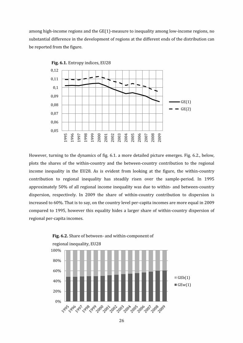
Figure 6.1, below, plots the GE(1)- and GE(2)-indices of regional per-capita GRP of the EU28-set
over the 1995-2009 period. As can be seen, besides the period 1997-2000, when inequality
increased somewhat, regional per-capita income inequality has steadily fallen over the period. In
other words, according to the indices there is less inter-distributional dispersion in regional
incomes in 2009 than in 1995. As the GE(2)-measure should be more sensitive to inequality
12 For a more detailed discussion of generalized entropy indices see Appendix III.
26
among high-income regions and the GE(1)-measure to inequality among low-income regions, no
substantial difference in the development of regions at the different ends of the distribution can
be reported from the figure.
However, turning to the dynamics of fig. 6.1. a more detailed picture emerges. Fig. 6.2., below,
plots the shares of the within-country and the between-country contribution to the regional
income inequality in the EU28. As is evident from looking at the figure, the within-country
contribution to regional inequality has steadily risen over the sample-period. In 1995
approximately 50% of all regional income inequality was due to within- and between-country
dispersion, respectively. In 2009 the share of within-country contribution to dispersion is
increased to 60%. That is to say, on the country level per-capita incomes are more equal in 2009
compared to 1995, however this equality hides a larger share of within-country dispersion of
regional per-capita incomes.
0,05
0,06
0,07
0,08
0,09
0,1
0,11
0,12
19
95
19
96
19
97
19
98
19
99
20
00
20
01
20
02
20
03
20
04
20
05
20
06
20
07
20
08
20
09
Fig. 6.1. Entropy indices, EU28
GE(1)
GE(2)
0%
20%
40%
60%
80%
100%
Fig. 6.2. Share of between- and within-component of
regional inequality, EU28
GEb(1)
GEw(1)

27
Taken together with fig. 6.1., fig. 6.2. paints a picture of decreasing regional income disparities.
However, this reduction is accompanied by a relative increase of the importance of within-
country inequality. In other words, a larger portion of the still existing inequality in the EU
seems to be due to inequality within countries. It is possible that these results pick up on the
findings reported above (Ezcurra et al. 2007b; Geppert and Stephen 2008; Chapman and
Melciani 2011; Paas and Schlitte 2007, 2008) of σ-convergence but increasing within-country
dispersion of regional incomes. If this is the case, what is driving the decreased inequality in the
EU28 on the country-level is the behavior of a few high-income regions among the NMS, who has
converged to the EU28-mean, leaving laggard low-income regions behind. This would certainly
explain why within-country inequality has increased, while overall inequality decreased.
To further investigate if there is any difference in the behavior of regions among the NMS and
the rest of the EU, the EU28-set is divided into a subset consisting of the EU15-regions and one
consisting of NMS-regions. First in fig. 6.3., below, the GE(1) and GE(2) inequality measures of
the EU15 over the sample-period is plotted. As can be seen, the development of regional income
inequality is generally stable in the subset, lessening somewhat over the period. What can be
noted is that the GE(1)-measure has decreased relatively more than the GE(2)-measure. Since
the GE(1)-measure should be more sensitive to dispersion among regional incomes in the lower
tail of the income distribution, it is possible that inequality among low-income regions has
decreased somewhat more relative inequality among high-income regions in the EU15.
Now, consider the shares of between- and within-country contribution to overall income
inequality in the EU15. Below fig. 6.4. shows how the lion’s share of regional income inequality
in the EU15 is made up of within-country dispersion. In other words, the EU15-countries show
somewhat equal per-capita income levels across countries, while the dispersion of regional
0,05
0,055
0,06
0,065
0,07
0,075
19
95
19
96
19
97
19
98
19
99
20
00
20
01
20
02
20
03
20
04
20
05
20
06
20
07
20
08
20
09
Fig. 6.3. Entropy indices, EU15
GE(1)
GE(2)
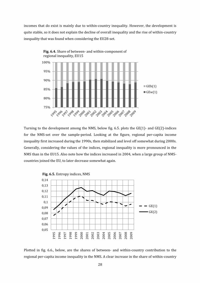
28
incomes that do exist is mainly due to within-country inequality. However, the development is
quite stable, so it does not explain the decline of overall inequality and the rise of within-country
inequality that was found when considering the EU28-set.
Turning to the development among the NMS, below fig. 6.5. plots the GE(1)- and GE(2)-indices
for the NMS-set over the sample-period. Looking at the figure, regional per-capita income
inequality first increased during the 1990s, then stabilized and level off somewhat during 2000s.
Generally, considering the values of the indices, regional inequality is more pronounced in the
NMS than in the EU15. Also note how the indices increased in 2004, when a large group of NMS-
countries joined the EU, to later decrease somewhat again.
Plotted in fig. 6.6., below, are the shares of between- and within-country contribution to the
regional per-capita income inequality in the NMS. A clear increase in the share of within-country
75%
80%
85%
90%
95%
100%
Fig. 6.4. Share of between- and within-component of regional inequality, EU15
GEb(1)
GEw(1)
0,05
0,06
0,07
0,08
0,09
0,1
0,11
0,12
0,13
0,14
19
95
19
96
19
97
19
98
19
99
20
00
20
01
20
02
20
03
20
04
20
05
20
06
20
07
20
08
20
09
Fig. 6.5. Entropy indices, NMS
GE(1)
GE(2)
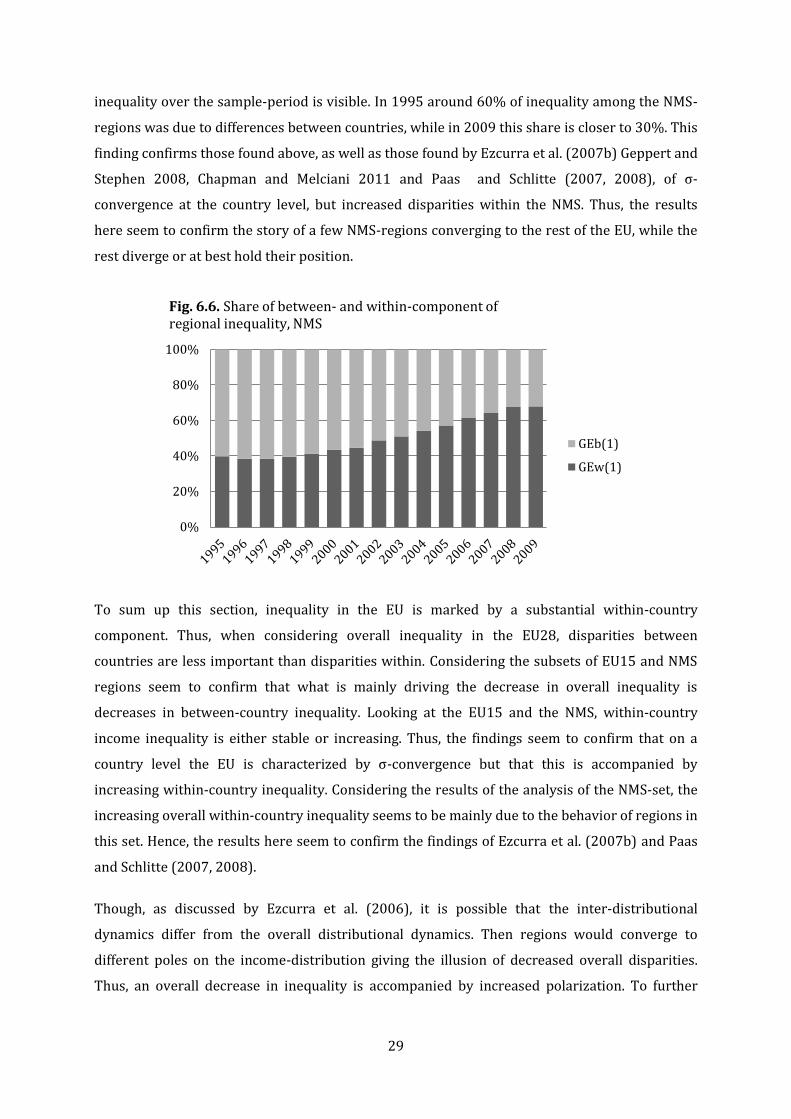
29
inequality over the sample-period is visible. In 1995 around 60% of inequality among the NMS-
regions was due to differences between countries, while in 2009 this share is closer to 30%. This
finding confirms those found above, as well as those found by Ezcurra et al. (2007b) Geppert and
Stephen 2008, Chapman and Melciani 2011 and Paas and Schlitte (2007, 2008), of σ-
convergence at the country level, but increased disparities within the NMS. Thus, the results
here seem to confirm the story of a few NMS-regions converging to the rest of the EU, while the
rest diverge or at best hold their position.
To sum up this section, inequality in the EU is marked by a substantial within-country
component. Thus, when considering overall inequality in the EU28, disparities between
countries are less important than disparities within. Considering the subsets of EU15 and NMS
regions seem to confirm that what is mainly driving the decrease in overall inequality is
decreases in between-country inequality. Looking at the EU15 and the NMS, within-country
income inequality is either stable or increasing. Thus, the findings seem to confirm that on a
country level the EU is characterized by σ-convergence but that this is accompanied by
increasing within-country inequality. Considering the results of the analysis of the NMS-set, the
increasing overall within-country inequality seems to be mainly due to the behavior of regions in
this set. Hence, the results here seem to confirm the findings of Ezcurra et al. (2007b) and Paas
and Schlitte (2007, 2008).
Though, as discussed by Ezcurra et al. (2006), it is possible that the inter-distributional
dynamics differ from the overall distributional dynamics. Then regions would converge to
different poles on the income-distribution giving the illusion of decreased overall disparities.
Thus, an overall decrease in inequality is accompanied by increased polarization. To further
0%
20%
40%
60%
80%
100%
Fig. 6.6. Share of between- and within-component of regional inequality, NMS
GEb(1)
GEw(1)
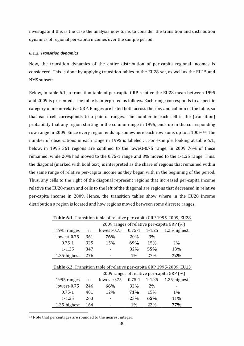
30
investigate if this is the case the analysis now turns to consider the transition and distribution
dynamics of regional per-capita incomes over the sample period.
6.1.2. Transition dynamics
Now, the transition dynamics of the entire distribution of per-capita regional incomes is
considered. This is done by applying transition tables to the EU28-set, as well as the EU15 and
NMS subsets.
Below, in table 6.1., a transition table of per-capita GRP relative the EU28-mean between 1995
and 2009 is presented. The table is interpreted as follows. Each range corresponds to a specific
category of mean-relative GRP. Ranges are listed both across the row and column of the table, so
that each cell corresponds to a pair of ranges. The number in each cell is the (transition)
probability that any region starting in the column range in 1995, ends up in the corresponding
row range in 2009. Since every region ends up somewhere each row sums up to a 100%13. The
number of observations in each range in 1995 is labeled n. For example, looking at table 6.1.,
below, in 1995 361 regions are confined to the lowest-0.75 range, in 2009 76% of these
remained, while 20% had moved to the 0.75-1 range and 3% moved to the 1-1.25 range. Thus,
the diagonal (marked with bold text) is interpreted as the share of regions that remained within
the same range of relative per-capita income as they began with in the beginning of the period.
Thus, any cells to the right of the diagonal represent regions that increased per-capita income
relative the EU28-mean and cells to the left of the diagonal are regions that decreased in relative
per-capita income in 2009. Hence, the transition tables show where in the EU28 income
distribution a region is located and how regions moved between some discrete ranges.
Table 6.1. Transition table of relative per-capita GRP 1995-2009, EU28
2009 ranges of relative per-capita GRP (%)
1995 ranges n lowest-0.75 0.75-1 1-1.25 1.25-highest
lowest-0.75 361 76% 20% 3% -
0.75-1 325 15% 69% 15% 2%
1-1.25 347 - 32% 55% 13%
1.25-highest 276 - 1% 27% 72%
Table 6.2. Transition table of relative per-capita GRP 1995-2009, EU15
2009 ranges of relative per-capita GRP (%)
1995 ranges n lowest-0.75 0.75-1 1-1.25 1.25-highest
lowest-0.75 246 66% 32% 2% -
0.75-1 401 12% 71% 15% 1%
1-1.25 263 - 23% 65% 11%
1.25-highest 164 - 1% 22% 77%
13 Note that percentages are rounded to the nearest integer.
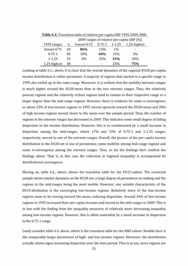
31
Table 6.3. Transition table of relative per-capita GRP 1995-2009, NMS
2009 ranges of relative per-capita GRP (%)
1995 ranges n lowest-0.75 0.75-1 1-1.25 1.25-highest
lowest-0.75 69 86% 13% 1% -
0.75-1 85 20% 60% 15% 5%
1-1.25 33 3% 33% 33% 30%
1.25-highest 48 - - 25% 75%
Looking at table 6.1., above, it is clear that the overall dynamics of the regional EU28 per-capita
income distribution is rather persistent. A majority of regions that started in a specific range in
1995 also ended up in the same range. Moreover, it is evident that the mobility between ranges
is much higher around the EU28-mean than in the two extreme ranges. Thus, the relatively
poorest regions and the relatively richest regions tend to remain in their respective range to a
larger degree than the mid-range regions. However, there is evidence for some σ-convergence,
as about 23% of low-income regions in 1995 moved upwards toward the EU28-mean and 28%
of high-income regions moved closer to the mean over the sample period. Thus, the number of
regions in the extreme ranges has decreased in 2009. This indicates some small degree of falling
dispersion in the income distribution. However, this is to counteracted by a small increase in
dispersion among the mid-ranges, where 17% and 13% of 0.75-1 and 1-1.25 ranges,
respectively, moved to one of the extreme ranges. Overall, the picture of the per-capita income
distribution in the EU28-set is one of persistence, some mobility among mid-range regions and
some σ-convergence among the extreme ranges. Thus, so far the findings here confirm the
findings above. That is, in this case the reduction in regional inequality is accompanied by
distributional convergence.
Moving on, table 6.2., above, shows the transition table for the EU15-subset. The restricted
sample shows similar dynamics as the EU28-set, a large degree of persistence in ranking and the
regions in the mid-ranges being the most mobile. However, one notable characteristic of the
EU15-ditribution is the converging low-income regions. Relatively more of the low-income
regions seem to be moving toward the mean, reducing disparities. Around 34% of low-income
regions in 1995 increased their per-capita incomes and moved to the mid-ranges in 2009. This is
in line with the finding from the inequality measures of relatively more decreasing inequality
among low-income regions. However, this is offset somewhat by a small increase in dispersion
in the 0.75-1 range.
Lastly consider table 6.3. above, which is the transition table for the NMS subset. Notable here is
the comparably larger persistence of high- and low-income regions. Moreover, the distribution
actually shows signs increasing disparities over the time period. That is to say, more regions are
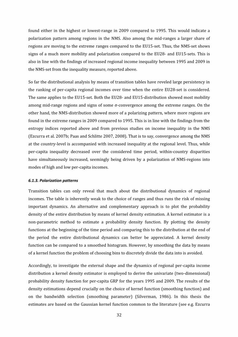
32
found either in the highest or lowest-range in 2009 compared to 1995. This would indicate a
polarization pattern among regions in the NMS. Also among the mid-ranges a larger share of
regions are moving to the extreme ranges compared to the EU15-set. Thus, the NMS-set shows
signs of a much more mobility and polarization compared to the EU28- and EU15-sets. This is
also in line with the findings of increased regional income inequality between 1995 and 2009 in
the NMS-set from the inequality measure, reported above.
So far the distributional analysis by means of transition tables have reveled large persistency in
the ranking of per-capita regional incomes over time when the entire EU28-set is considered.
The same applies to the EU15-set. Both the EU28- and EU15-distribution showed most mobility
among mid-range regions and signs of some σ-convergence among the extreme ranges. On the
other hand, the NMS-distribution showed more of a polarizing pattern, where more regions are
found in the extreme ranges in 2009 compared to 1995. This is in line with the findings from the
entropy indices reported above and from previous studies on income inequality in the NMS
(Ezcurra et al. 2007b; Paas and Schlitte 2007, 2008). That is to say, convergence among the NMS
at the country-level is accompanied with increased inequality at the regional level. Thus, while
per-capita inequality decreased over the considered time period, within-country disparities
have simultaneously increased, seemingly being driven by a polarization of NMS-regions into
modes of high and low per-capita incomes.
6.1.3. Polarization patterns
Transition tables can only reveal that much about the distributional dynamics of regional
incomes. The table is inherently weak to the choice of ranges and thus runs the risk of missing
important dynamics. An alternative and complementary approach is to plot the probability
density of the entire distribution by means of kernel density estimation. A kernel estimator is a
non-parametric method to estimate a probability density function. By plotting the density
functions at the beginning of the time period and comparing this to the distribution at the end of
the period the entire distributional dynamics can better be appreciated. A kernel density
function can be compared to a smoothed histogram. However, by smoothing the data by means
of a kernel function the problem of choosing bins to discretely divide the data into is avoided.
Accordingly, to investigate the external shape and the dynamics of regional per-capita income
distribution a kernel density estimator is employed to derive the univariate (two-dimensional)
probability density function for per-capita GRP for the years 1995 and 2009. The results of the
density estimations depend crucially on the choice of kernel function (smoothing function) and
on the bandwidth selection (smoothing parameter) (Silverman, 1986). In this thesis the
estimates are based on the Gaussian kernel function common to the literature (see e.g. Ezcurra
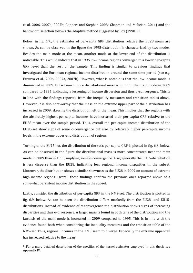
33
et al. 2006, 2007a, 2007b; Geppert and Stephan 2008; Chapman and Meliciani 2011) and the
bandwidth selection follows the adaptive method suggested by Fox (1990).14
Below, in fig. 6.7., the estimates of per-capita GRP distribution relative the EU28 mean are
shown. As can be observed in the figure the 1995-distribution is characterized by two modes.
Besides the main mode at the mean, another mode at the lower-end of the distribution is
noticeable. This would indicate that in 1995 low-income regions converged to a lower per-capita
GRP level than the rest of the sample. This finding is similar to previous findings that
investigated the European regional income distribution around the same time period (see e.g.
Ezcurra et al., 2006, 2007a, 2007b). However, what is notable is that the low-income mode is
diminished in 2009. In fact much more distributional mass is found in the main mode in 2009
compared to 1995, indicating a lessening of income dispersion and thus σ-convergence. This is
in line with the findings reported from the inequality measures and transition tables above.
However, it is also noteworthy that the mass on the extreme upper part of the distribution has
increased in 2009, skewing the distribution left of the mean. This implies that the regions with
the absolutely highest per-capita incomes have increased their per-capita GRP relative to the
EU28-mean over the sample period. Thus, overall the per-capita income distribution of the
EU28-set show signs of some σ-convergence but also by relatively higher per-capita income
levels in the extreme upper-end distribution of regions.
Turning to the EU15-set, the distribution of the set’s per-capita GRP is plotted in fig. 6.8, below.
As can be observed in the figure the distributional mass is more concentrated near the main
mode in 2009 than in 1995, implying some σ-convergence. Also, generally the EU15-distribution
is less disperse than the EU28, indicating less regional income disparities in the subset.
Moreover, the distribution shows a similar skewness as the EU28 in 2009 on account of extreme
high-income regions. Overall these findings confirm the previous ones reported above of a
somewhat persistent income distribution in the subset.
Lastly, consider the distribution of per-capita GRP in the NMS-set. The distribution is plotted in
fig. 6.9. below. As can be seen the distribution differs markedly from the EU28- and EU15-
distributions. Instead of evidence of σ-convergence the distribution shows signs of increasing
disparities and thus σ-divergence. A larger mass is found in both tails of the distribution and the
kurtosis of the main mode is increased in 2009 compared to 1995. This is in line with the
evidence found both when considering the inequality measures and the transition table of the
NMS-set. Thus, regional incomes in the NMS seem to diverge. Especially the extreme upper-tail
has increased relative to the mean
14 For a more detailed description of the specifics of the kernel estimator employed in this thesis see Appendix IV.
34
Fig. 6.7. Density function for EU28 relative per-capita GRP 1995 and 2009
Fig. 6.8. Density function for EU15 relative per-capita GRP 1995 and 2009
0.5
11.5
0 1 2 3 4 5 6 7GRP per-capita, EU28=1
GRPpc1995 GRPpc2009
Note: Gaussian kernel with adaptive bandwidth
0.5
11.5
2
0 1 2 3 4 5 6GRP per-capita, EU15=1
GRPpc1995 GRPpc2009
Note: Gaussian kernel with adaptive bandwidth

35
Fig. 6.9. Density function for NMS relative per-capita GRP 1995 and 2009
To summarize the findings in the distributional analysis. Firstly, it can be noted that overall the
EU28 is marked by declining regional per-capita income inequality. However, the contribution of
within-country disparities to overall inequality has increased over the considered period.
Moreover, the decline in inequality is accompanied with a lessening of dispersion in the regional
per-capita income distribution, so that the entire EU28-set shows evidence of weak σ-
convergence. The EU15-set also shows evidence of declining inequality and distributional-
dispersion in per-capita incomes. Also striking about the regional income dynamics in the subset
is its persistence over the considered time period. One interpretation of these findings is that the
detected convergence is mainly due to income growth among low-income EU15-regions, while
high-income regions show a large degree of persistence. Also noteworthy of the EU15 is that
inequality in the subset is marked by a considerable within-country component. The dynamics
of NMS distribution differ from the EU15 in that it show signs of increasing income inequality
and dispersion of regional per-capita GRP over the sample period. Thus, per-capita income in the
NMS is more unevenly distributed across regions in 2009 compared to 1995. This finding is in
line with previous research. Hence, the decline in overall inequality reported in section 6.2.2.
seems to be mainly driven by σ-convergence in the distribution of EU15-regions. Furthermore,
this thesis finds no evidence of the bimodal or a multimodal polarization patterns reported in
several previous studies in section 3.2. Instead, a unimodal pole is found in all considered
distributions in 2009 and only the thickness of the tails of the distribution differs when
0.5
11.5
.5 1 1.5 2 2.5 3 3.5GRP per-capita, NMS=1
GRPpc1995 GRPpc2009
Note: Gaussian kernel with adaptive bandwidth
36
considering different regional sets. Thus it seems possible that the multimodality of the income
distribution has disappeared over time.
6.2. Exploratory spatial data analysis
The analysis now turns to consider the spatial dimension of the distribution of regional per-
capita incomes and growth rates. To do this exploratory spatial data analysis (ESDA) techniques
are used. Following Dall’erba (2005: p.126), ESDA is a set of techniques to describe, visualize
spatial distributions and to identify patterns of spatial clustering. Following Anselin (1988,
1995), in the subsequent analysis ESDA-techniques to detect spatial dependency over the entire
dataset (global spatial autocorrelation) and local clusters of spatial dependence (local spatial
autocorrelation) of both regional per-capita GRP and growth rates are employed. Spatial
autocorrelation is similar to temporal autocorrelation in that geographical units need not be
independent across space. However, while temporal autocorrelation is one-dimensional and
one-directional, spatial autocorrelation can be two-dimensional and multi-directional. By
measuring the spatial autocorrelation the degree of regional spatial dependence can be
estimated. A related topic is that of spatial heterogeneity, meaning that the spatial distribution is
uneven and bounded across space, so that local clusters of similar or dissimilar values emerge.
Thus, if regions of similar values in initial per-capita GRP or average growth rates are found to
be clustered together in space, this is interpreted as support for geographically conditioned
convergence-clubs.
6.2.1. Global spatial autocorrelation
Following Dall’erba (2005: p.130f.), spatial autocorrelation can be defined as a spatial clustering
of similar values of some variable. If similar values are clustered in space there is positive spatial
correlation. Conversely, dissimilar clustered values are interpreted as negative spatial
autocorrelation. To measure the spatial autocorrelation in the dataset Moran’s I statistic is
computed (Moran, 1950). This statistic captures global spatial autocorrelation of the variables of
interest.
Specifically, the Moran’s I statistic for region i is given by,
∑ ∑
∑ ∑
∑
, (6.1)
where is the ijth-element of the specified spatial-weight matrix 15, is the variable of
interest in region i and is the mean of this variable, so that the variable is expressed as mean-
15 The spatial weight matrix is defined in Appendix I.
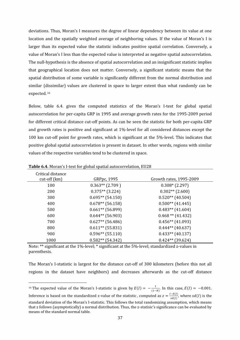
37
deviations. Thus, Moran’s I measures the degree of linear dependency between its value at one
location and the spatially weighted average of neighboring values. If the value of Moran’s I is
larger than its expected value the statistic indicates positive spatial correlation. Conversely, a
value of Moran’s I less than the expected value is interpreted as negative spatial autocorrelation.
The null-hypothesis is the absence of spatial autocorrelation and an insignificant statistic implies
that geographical location does not matter. Conversely, a significant statistic means that the
spatial distribution of some variable is significantly different from the normal distribution and
similar (dissimilar) values are clustered in space to larger extent than what randomly can be
expected. 16
Below, table 6.4. gives the computed statistics of the Moran’s I-test for global spatial
autocorrelation for per-capita GRP in 1995 and average growth rates for the 1995-2009 period
for different critical distance cut-off points. As can be seen the statistic for both per-capita GRP
and growth rates is positive and significant at 1%-level for all considered distances except the
100 km cut-off point for growth rates, which is significant at the 5%-level. This indicates that
positive global spatial autocorrelation is present in dataset. In other words, regions with similar
values of the respective variables tend to be clustered in space.
Table 6.4. Moran's I-test for global spatial autocorrelation, EU28
Critical distance cut-off (km) GRPpc, 1995 Growth rates, 1995-2009
100 0.363** (2.709 ) 0.308* (2.297)
200 0.375** (3.224) 0.302** (2.600)
300 0.695** (54.150) 0.520** (40.504)
400 0.678** (56.158) 0.500** (41.445)
500 0.661** (56.899) 0.483** (41.604)
600 0.644** (56.903) 0.468 ** (41.432)
700 0.627** (56.486) 0.456** (41.093)
800 0.611** (55.831) 0.444** (40.637)
900 0.596** (55.110) 0.433** (40.137)
1000 0.582** (54.342) 0.424** (39.624)
Note: ** significant at the 1%-level; * significant at the 5%-level; standardized z-values in parenthesis.
The Moran’s I-statistic is largest for the distance cut-off of 300 kilometers (before this not all
regions in the dataset have neighbors) and decreases afterwards as the cut-off distance
16 The expected value of the Moran’s I-statistic is given by
. In this case, .
Inference is based on the standardized z-value of the statistic , computed as
, where is the
standard deviation of the Moran’s I-statistic. This follows the total randomizing assumption, which means that z follows (asymptotically) a normal distribution. Thus, the z-statisic’s significance can be evaluated by means of the standard normal table.
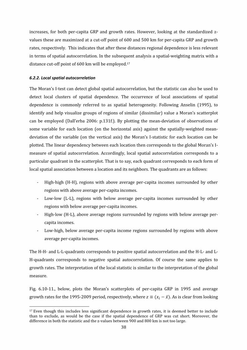
38
increases, for both per-capita GRP and growth rates. However, looking at the standardized z-
values these are maximized at a cut-off point of 600 and 500 km for per-capita GRP and growth
rates, respectively. This indicates that after these distances regional dependence is less relevant
in terms of spatial autocorrelation. In the subsequent analysis a spatial-weighting matrix with a
distance cut-off point of 600 km will be employed.17
6.2.2. Local spatial autocorrelation
The Moran’s I-test can detect global spatial autocorrelation, but the statistic can also be used to
detect local clusters of spatial dependence. The occurrence of local associations of spatial
dependence is commonly referred to as spatial heterogeneity. Following Anselin (1995), to
identify and help visualize groups of regions of similar (dissimilar) value a Moran’s scatterplot
can be employed (Dall’erba 2006: p.131f.). By plotting the mean-deviation of observations of
some variable for each location (on the horizontal axis) against the spatially-weighted mean-
deviation of the variable (on the vertical axis) the Moran’s I-statistic for each location can be
plotted. The linear dependency between each location then corresponds to the global Moran’s I-
measure of spatial autocorrelation. Accordingly, local spatial autocorrelation corresponds to a
particular quadrant in the scatterplot. That is to say, each quadrant corresponds to each form of
local spatial association between a location and its neighbors. The quadrants are as follows:
- High-high (H-H), regions with above average per-capita incomes surrounded by other
regions with above average per-capita incomes.
- Low-low (L-L), regions with below average per-capita incomes surrounded by other
regions with below average per-capita incomes.
- High-low (H-L), above average regions surrounded by regions with below average per-
capita incomes.
- Low-high, below average per-capita income regions surrounded by regions with above
average per-capita incomes.
The H-H- and L-L-quadrants corresponds to positive spatial autocorrelation and the H-L- and L-
H-quadrants corresponds to negative spatial autocorrelation. Of course the same applies to
growth rates. The interpretation of the local statistic is similar to the interpretation of the global
measure.
Fig. 6.10-11., below, plots the Moran’s scatterplots of per-capita GRP in 1995 and average
growth rates for the 1995-2009 period, respectively, where . As is clear from looking
17 Even though this includes less significant dependence in growth rates, it is deemed better to include than to exclude, as would be the case if the spatial dependence of GRP was cut short. Moreover, the difference in both the statistic and the z-values between 900 and 800 km is not too large.
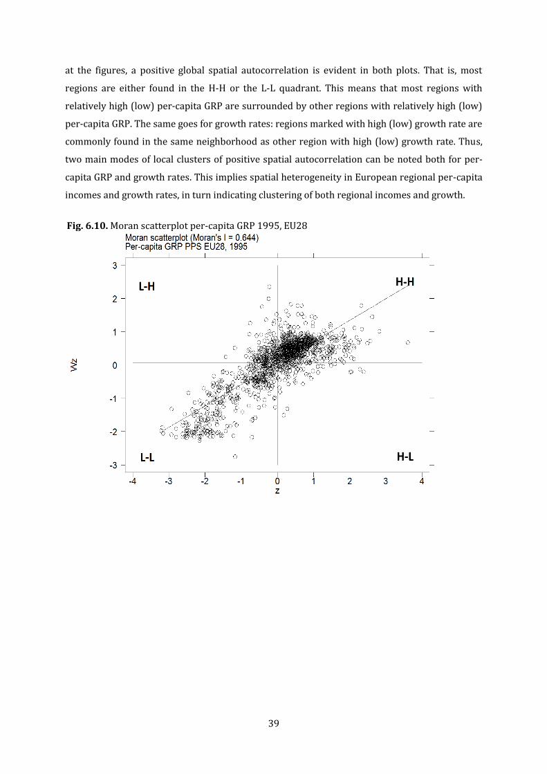
39
at the figures, a positive global spatial autocorrelation is evident in both plots. That is, most
regions are either found in the H-H or the L-L quadrant. This means that most regions with
relatively high (low) per-capita GRP are surrounded by other regions with relatively high (low)
per-capita GRP. The same goes for growth rates: regions marked with high (low) growth rate are
commonly found in the same neighborhood as other region with high (low) growth rate. Thus,
two main modes of local clusters of positive spatial autocorrelation can be noted both for per-
capita GRP and growth rates. This implies spatial heterogeneity in European regional per-capita
incomes and growth rates, in turn indicating clustering of both regional incomes and growth.
Fig. 6.10. Moran scatterplot per-capita GRP 1995, EU28
40
Fig. 6.11. Moran scatterplot growth rates 1995-2009, EU28
Following Anselin (1995), to investigate the geography of the detected spatial heterogeneity the
local Moran’s I for each region’s per-capita GRP in 1995 and average growth rate for the period
is computed and the results are plotted on maps, see fig. 6.12-13, below. The maps show
significant clusters of local Moran’s I-statistics at the 5%-level.
First, in fig. 6.12, note the positive spatial correlation of high per-capita GRP in the geographical
centre of the EU. That is, Austria, Germany, France, Northern Italy, Denmark and partly Great
Britain and Sweden all show evidence of clustering of positive spatial autocorrelation of
relatively high regional incomes. Conversely, among peripheral regions, the NMS as well as part
of Spain, Portugal, Southern Italy and Greece, evidence points to clustering of positive spatial
autocorrelation of relatively low values of relative per-capita GRP. Polish regions make up the
only larger cluster of negative spatial autocorrelation, showing significant low-high clustering.
The interpretation of this is straightforward, Poland, a relative low per-capita income country, is
the neighbor of Germany, a relatively high per-capita income country.
The divide between a core and periphery in Europe becomes even clearer when considering
growth rates. Looking at figure 6.13. with few exceptions, the regional neighborhoods that
exhibited relatively high per-capita incomes in 1995 have exhibited relatively lower average
growth rate in subsequent years. Figure 6.13. is almost the inverse of figure 5.12. A notable
exception is the Netherlands that constitute a relatively high-income cluster that also appears to
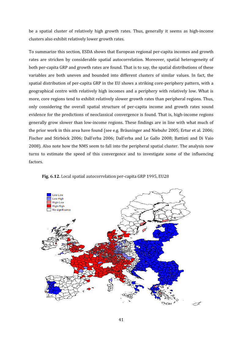
41
be a spatial cluster of relatively high growth rates. Thus, generally it seems as high-income
clusters also exhibit relatively lower growth rates.
To summarize this section, ESDA shows that European regional per-capita incomes and growth
rates are stricken by considerable spatial autocorrelation. Moreover, spatial heterogeneity of
both per-capita GRP and growth rates are found. That is to say, the spatial distributions of these
variables are both uneven and bounded into different clusters of similar values. In fact, the
spatial distribution of per-capita GRP in the EU shows a striking core-periphery pattern, with a
geographical centre with relatively high incomes and a periphery with relatively low. What is
more, core regions tend to exhibit relatively slower growth rates than peripheral regions. Thus,
only considering the overall spatial structure of per-capita income and growth rates sound
evidence for the predictions of neoclassical convergence is found. That is, high-income regions
generally grow slower than low-income regions. These findings are in line with what much of
the prior work in this area have found (see e.g. Bräuninger and Niebuhr 2005; Ertur et al. 2006;
Fischer and Stirböck 2006; Dall’erba 2006; Dall’erba and Le Gallo 2008; Battisti and Di Vaio
2008). Also note how the NMS seem to fall into the peripheral spatial cluster. The analysis now
turns to estimate the speed of this convergence and to investigate some of the influencing
factors.
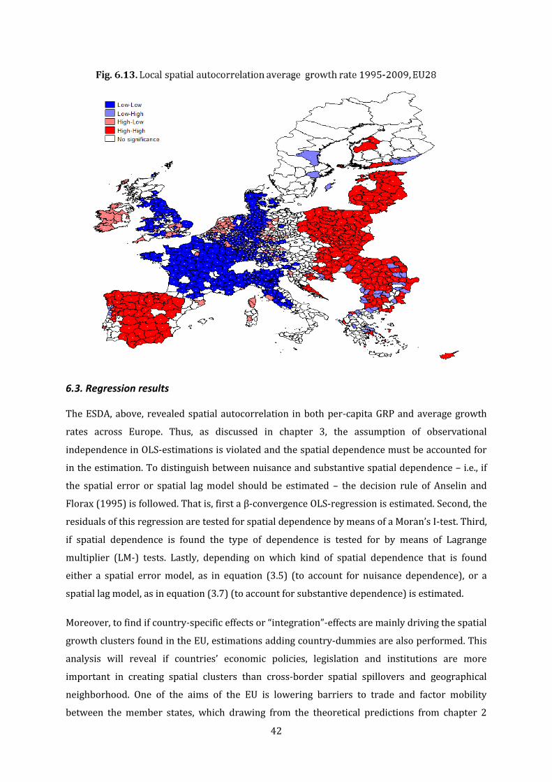
42
6.3. Regression results
The ESDA, above, revealed spatial autocorrelation in both per-capita GRP and average growth
rates across Europe. Thus, as discussed in chapter 3, the assumption of observational
independence in OLS-estimations is violated and the spatial dependence must be accounted for
in the estimation. To distinguish between nuisance and substantive spatial dependence – i.e., if
the spatial error or spatial lag model should be estimated – the decision rule of Anselin and
Florax (1995) is followed. That is, first a β-convergence OLS-regression is estimated. Second, the
residuals of this regression are tested for spatial dependence by means of a Moran’s I-test. Third,
if spatial dependence is found the type of dependence is tested for by means of Lagrange
multiplier (LM-) tests. Lastly, depending on which kind of spatial dependence that is found
either a spatial error model, as in equation (3.5) (to account for nuisance dependence), or a
spatial lag model, as in equation (3.7) (to account for substantive dependence) is estimated.
Moreover, to find if country-specific effects or “integration”-effects are mainly driving the spatial
growth clusters found in the EU, estimations adding country-dummies are also performed. This
analysis will reveal if countries’ economic policies, legislation and institutions are more
important in creating spatial clusters than cross-border spatial spillovers and geographical
neighborhood. One of the aims of the EU is lowering barriers to trade and factor mobility
between the member states, which drawing from the theoretical predictions from chapter 2
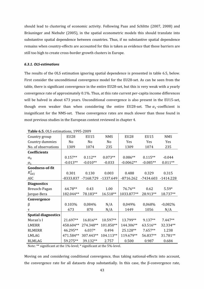
43
should lead to clustering of economic activity. Following Paas and Schlitte (2007, 2008) and
Bräuninger and Niebuhr (2005), in the spatial econometric models this should translate into
substantive spatial dependence between countries. Thus, if no substantive spatial dependence
remains when country-effects are accounted for this is taken as evidence that those barriers are
still too high to create cross-border growth clusters in Europe.
6.3.1. OLS-estimations
The results of the OLS estimation ignoring spatial dependence is presented in table 6.5, below.
First consider the unconditional convergence model for the EU28-set. As can be seen from the
table, there is significant convergence in the entire EU28-set, but this is very weak with a yearly
convergence rate of approximately 0.1%. Thus, at this rate current per-capita income differences
will be halved in about 673 years. Unconditional convergence is also present in the EU15-set,
though even weaker than when considering the entire EU28-set. The -coefficient is
insignificant for the NMS-set. These convergence rates are much slower than those found in
most previous studies in the European context reviewed in chapter 4.
Table 6.5. OLS estimations, 1995-2009
Country group EU28 EU15 NMS EU28 EU15 NMS
Country dummies No No No Yes Yes Yes
No. of observations 1309 1074 235 1309 1074 235
Coefficients
0.157** 0.112** 0.073** 0.086** 0.115** -0.044
-0.013** -0.010** -0.033 -0.0062** -0.085** 0.011**
Goodness-of-fit
0.301 0.130 0.003 0.488 0.329 0.315
AIC -8333.837 -7168.729 -1337.649 -8716.262 -7434.603 -1414.228
Diagnostics
Breusch-Pagan 64.78** 0.43 1.00 76.76** 0.62 5.59*
Jarque-Bera 182.044** 78.183** 16.518** 1033.877** 28.913** 18.737**
Convergence
β 0.103% 0,084% N/A 0,049% 0,068% -0,082%
τ 673 870 N/A 1449 1056 N/A
Spatial diagnostics
Moran's I 21.697** 16.816** 10.597** 13.799** 9.137** 7.447**
LMERR 458.604** 274.348** 101.850** 144.306** 63.516** 32.334**
RLMERR 46.295** 6.037* 0.494 25.128** 7.657** 1.238
LMLAG 471.584** 307.443** 104.113** 119.679** 56.837** 31.781**
RLMLAG 59.275** 39.132** 2.757 0.500 0.987 0.684
Note: ** significant at the 1%-level; * significant at the 5%-level.
Moving on and considering conditional convergence, thus taking national-effects into account,
the convergence rate for all datasets drop substantially. In this case, the β-convergence rate,
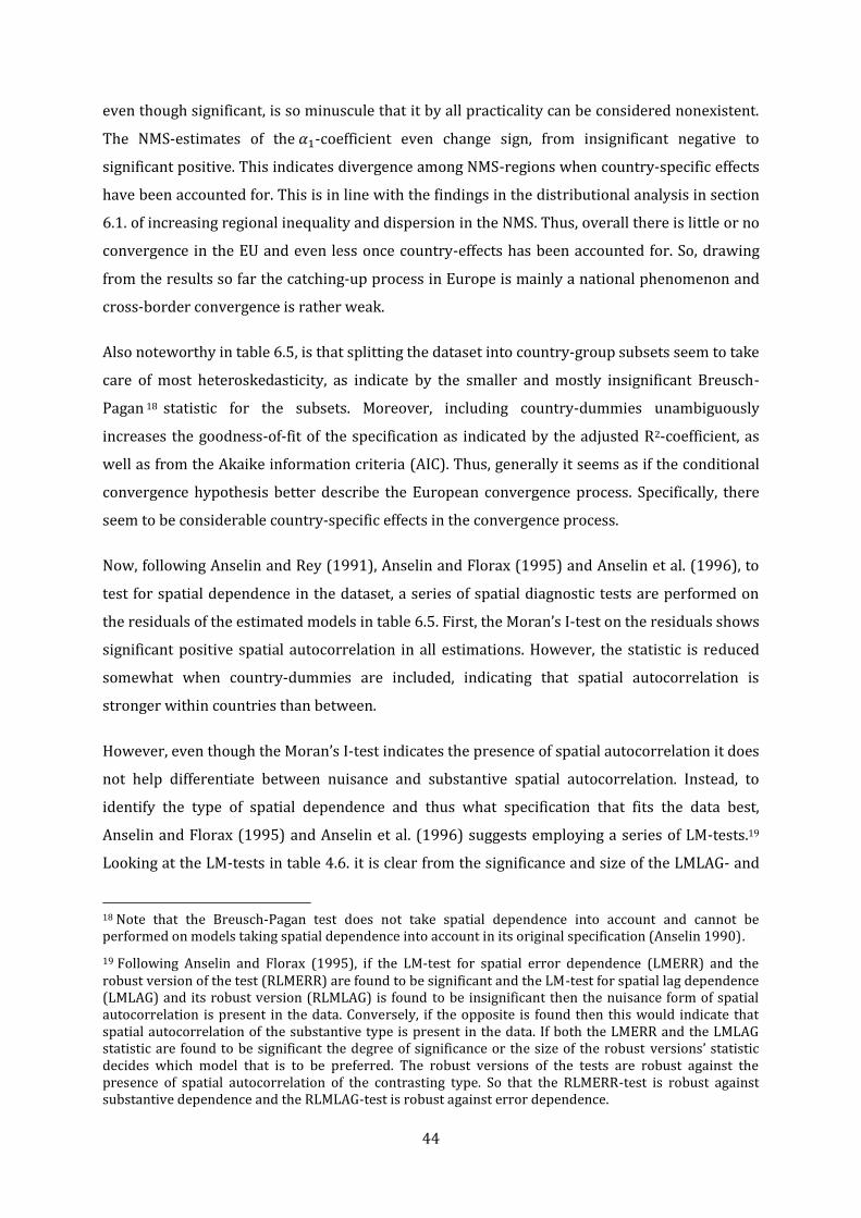
44
even though significant, is so minuscule that it by all practicality can be considered nonexistent.
The NMS-estimates of the -coefficient even change sign, from insignificant negative to
significant positive. This indicates divergence among NMS-regions when country-specific effects
have been accounted for. This is in line with the findings in the distributional analysis in section
6.1. of increasing regional inequality and dispersion in the NMS. Thus, overall there is little or no
convergence in the EU and even less once country-effects has been accounted for. So, drawing
from the results so far the catching-up process in Europe is mainly a national phenomenon and
cross-border convergence is rather weak.
Also noteworthy in table 6.5, is that splitting the dataset into country-group subsets seem to take
care of most heteroskedasticity, as indicate by the smaller and mostly insignificant Breusch-
Pagan 18 statistic for the subsets. Moreover, including country-dummies unambiguously
increases the goodness-of-fit of the specification as indicated by the adjusted R2-coefficient, as
well as from the Akaike information criteria (AIC). Thus, generally it seems as if the conditional
convergence hypothesis better describe the European convergence process. Specifically, there
seem to be considerable country-specific effects in the convergence process.
Now, following Anselin and Rey (1991), Anselin and Florax (1995) and Anselin et al. (1996), to
test for spatial dependence in the dataset, a series of spatial diagnostic tests are performed on
the residuals of the estimated models in table 6.5. First, the Moran’s I-test on the residuals shows
significant positive spatial autocorrelation in all estimations. However, the statistic is reduced
somewhat when country-dummies are included, indicating that spatial autocorrelation is
stronger within countries than between.
However, even though the Moran’s I-test indicates the presence of spatial autocorrelation it does
not help differentiate between nuisance and substantive spatial autocorrelation. Instead, to
identify the type of spatial dependence and thus what specification that fits the data best,
Anselin and Florax (1995) and Anselin et al. (1996) suggests employing a series of LM-tests.19
Looking at the LM-tests in table 4.6. it is clear from the significance and size of the LMLAG- and
18 Note that the Breusch-Pagan test does not take spatial dependence into account and cannot be performed on models taking spatial dependence into account in its original specification (Anselin 1990).
19 Following Anselin and Florax (1995), if the LM-test for spatial error dependence (LMERR) and the robust version of the test (RLMERR) are found to be significant and the LM-test for spatial lag dependence (LMLAG) and its robust version (RLMLAG) is found to be insignificant then the nuisance form of spatial autocorrelation is present in the data. Conversely, if the opposite is found then this would indicate that spatial autocorrelation of the substantive type is present in the data. If both the LMERR and the LMLAG statistic are found to be significant the degree of significance or the size of the robust versions’ statistic decides which model that is to be preferred. The robust versions of the tests are robust against the presence of spatial autocorrelation of the contrasting type. So that the RLMERR-test is robust against substantive dependence and the RLMLAG-test is robust against error dependence.
45
RLMLAG-statistic that substantive spatial autocorrelation is present in the unconditional model
in both the EU28-set and the EU15-set. For the NMS-set neither the RLMERR nor the RLMLAG
are significant. Hence, the tests fail to distinguish between nuisance and substantive spatial
dependence in the NMS subset.
Next, considering the conditional convergence model, taking country-effects into account seem
to reverse the predictions of the LM-tests for both the EU28- and EU15-sets. Now, the RLMERR-
test shows a significant statistic and the RLMLAG-test show an insignificant statistic for both
sets. This can be interpreted as substantive spatial dependence mainly being a within-country
phenomenon. That is to say, substantive spatial spillovers seem to stop at national borders.
Then what remains between countries is mainly nuisance dependence. Moreover, note that the
size of all the LM test-statistics is smaller in all specifications with country-dummies. Thus,
overall spatial dependence is weaker between countries than within. However, at this point it is
important to note that in presence of non-normality the LM-tests can be unreliable. As can be
seen in table 5.5., the Jarque-Bera test detects non-normality in all specifications. Thus, the
reliability of the LM-tests can be questioned. Consequently, both the spatial error model (SEM)
and the spatial lag model (SLM) will be estimated for all datasets.
6.3.2. Spatial econometric estimations
Table 6.6-7., below, shows the estimates of the SEM and SLM specifications, respectively. First
looking at table 6.6. and the SEM-specification, the spatial error coefficient, , is significant and
positive, implying positive spatial error dependence in the EU28-set. That is, an unexpected
negative (positive) growth shock to a region will spread through the regional system, affecting
neighboring regions’ growth rates negatively (positively). Moreover, regional convergence is
still significant, but the rate of β-convergence is further reduced compared to the OLS-
estimations in table 6.6. The EU15-set shows similar evidence as the EU28-set. In the case of the
NMS, the -estimate is again insignificant. However, the spatial error coefficient is significantly
positive, indicating the importance of spatial error dependence also in the NMS-set. This is
further corroborated by the significant likelihood-ratio test, which tests whether is
significantly different from zero. Thus, if the spatial specifications are better fits than the OLS-
specifications. As can be seen from the significance of the LR-tests there seem to be spatial
dependence across all sets.
Moreover, according to the AIC-statistic, again the model taking country-effects into account
seem to explain the data better than no-country-effects model in table 6.6.20 What is more,
20 Note that the R2 in maximum likelihood estimation is a pseudo measure and not comparable to the R2 of the OLS model. Therefore, only the AIC is used at this point, as suggested by Anselin et al. (1996).
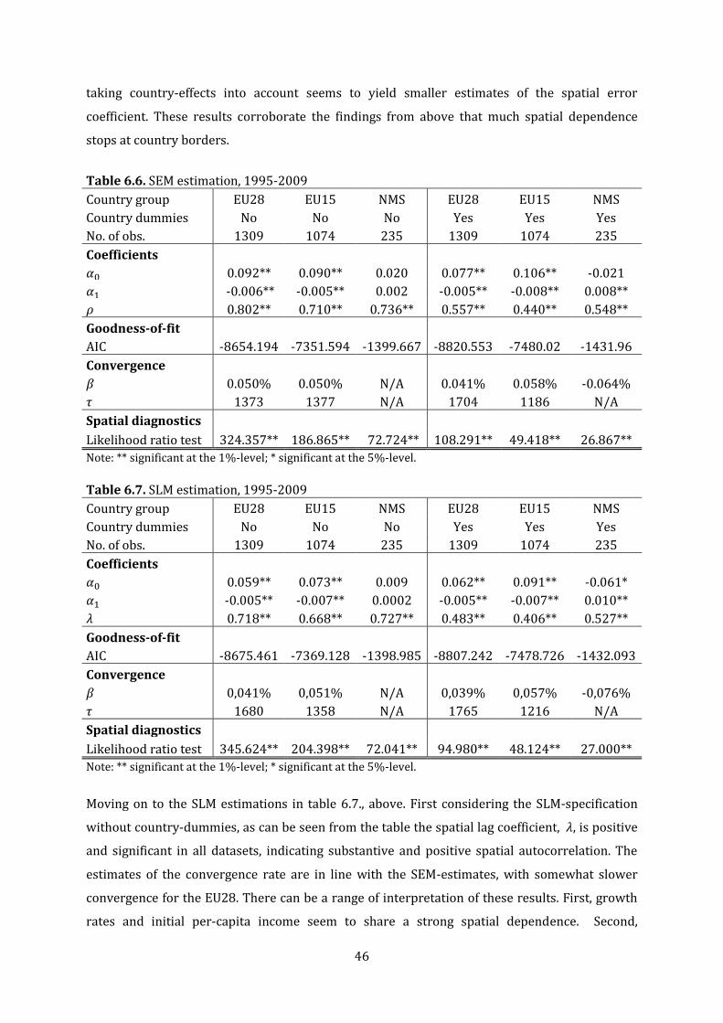
46
taking country-effects into account seems to yield smaller estimates of the spatial error
coefficient. These results corroborate the findings from above that much spatial dependence
stops at country borders.
Table 6.6. SEM estimation, 1995-2009
Country group EU28 EU15 NMS EU28 EU15 NMS
Country dummies No No No Yes Yes Yes
No. of obs. 1309 1074 235 1309 1074 235
Coefficients
0.092** 0.090** 0.020 0.077** 0.106** -0.021
-0.006** -0.005** 0.002 -0.005** -0.008** 0.008**
0.802** 0.710** 0.736** 0.557** 0.440** 0.548**
Goodness-of-fit
AIC -8654.194 -7351.594 -1399.667 -8820.553 -7480.02 -1431.96
Convergence
0.050% 0.050% N/A 0.041% 0.058% -0.064%
1373 1377 N/A 1704 1186 N/A
Spatial diagnostics
Likelihood ratio test 324.357** 186.865** 72.724** 108.291** 49.418** 26.867**
Note: ** significant at the 1%-level; * significant at the 5%-level.
Table 6.7. SLM estimation, 1995-2009
Country group EU28 EU15 NMS EU28 EU15 NMS
Country dummies No No No Yes Yes Yes
No. of obs. 1309 1074 235 1309 1074 235
Coefficients 0.059** 0.073** 0.009 0.062** 0.091** -0.061*
-0.005** -0.007** 0.0002 -0.005** -0.007** 0.010**
0.718** 0.668** 0.727** 0.483** 0.406** 0.527**
Goodness-of-fit AIC -8675.461 -7369.128 -1398.985 -8807.242 -7478.726 -1432.093
Convergence 0,041% 0,051% N/A 0,039% 0,057% -0,076%
1680 1358 N/A 1765 1216 N/A
Spatial diagnostics Likelihood ratio test 345.624** 204.398** 72.041** 94.980** 48.124** 27.000**
Note: ** significant at the 1%-level; * significant at the 5%-level.
Moving on to the SLM estimations in table 6.7., above. First considering the SLM-specification
without country-dummies, as can be seen from the table the spatial lag coefficient, , is positive
and significant in all datasets, indicating substantive and positive spatial autocorrelation. The
estimates of the convergence rate are in line with the SEM-estimates, with somewhat slower
convergence for the EU28. There can be a range of interpretation of these results. First, growth
rates and initial per-capita income seem to share a strong spatial dependence. Second,
47
convergence is less pronounced when spatial dependence is accounted for. Thus, with
neighborhood-effects the convergence rate is even slower. Taken together there seem to be a
large degree of spatial dependence between initial income and growth rates but not a strong
convergent relationship. Moreover, when comparing table 6.6 and 6.7 the AIC statistic indicates
an improved fit for the SLM-specification over the SEM-specification for all considered sets.
Next, when country dummies are included in the SLM-specification, the convergence rate drops
further. However, the size of the spatial lag coefficient is smaller compared to the no-country-
dummy case, again indicating that much substantive spatial dependence stops at national
borders. As above, the estimates for the NMS indicate significant but slow divergence when
country-effects have been accounted for.
Furthermore, comparing table 6.6 and 6.7, when country-effects are considered the preference
of the AIC and likelihood-ratio test change from above and the SEM is preferred over the SLM for
all sets except the NMS. However, the results for the NMS are not very substantial. This can be
taken as a confirmation of the results of the LM-test in the ordinary OLS-estimation above. That
is, substantive spatial dependence is mainly contained within countries. In other words, when
country-effects are accounted for the between-country dependence that remains is mainly of the
nuisance kind.
To summarize the findings from the regression analyses. First, for the EU28- and EU15-sets
there is very slow but significant convergence and not accounting for country-effects the results
favor the SLM-specification. Thus, there seem to be substantial regional spatial dependence in
the two sets. On the other hand, the no-country-dummy model for the NMS does not show any
evidence for convergence and the SEM specification is preferred. However, when country-effects
are accounted for, the conditional convergence models for the EU28- and EU15-set show
evidence of error dependence. This could indicate that substantive spatial dependence is mainly
contained to regions within the same country in these sets. Moreover, accounting for country-
effects further reduces the already slow convergence rate to a more or less nonexistent rate.
Conversely, in the NMS there do seem to be some substantive spatial dependence when country
effects have been controlled for. However, the differences between the estimates are not very
large. Moreover, in line with the findings in section 6.1 the NMS-set now show evidence for
divergent regional income growth trends.
7. Conclusions
The purpose of this thesis is firstly to extend on the prior works in the field of regional
convergence and spatial dependence in the EU. Secondly the thesis aims at investigating
48
differences in convergence dynamics between the EU15 and the NMS. Lastly, it considers if
spatial dependence in the regional convergence-process is mainly an artifact of country
affiliation or neighborhood. Regarding the first aim a comparably larger dataset with per-capita
GRP across NUTS 3-reigions is employed. In addition, the analysis is brought to a more recent
time period, namely 1995-2009. As in most recent studies in the field, ESDA-techniques and
spatial econometric methods are employed to account for spatial dependence. Moreover, two
commonly separated analytical strands, parametric β-convergence analysis and nonparametric
σ-convergence analysis, are brought together to give complementary analyses. To account for
different convergence dynamics in the EU15 and the NMS, the dataset is split into two subsets of
regions in accordance with the two groups
The unconditional convergence hypothesis of neoclassical theory predicts that poorer regions
will grow faster than richer ones, converging to the same income level. That is to say, regions are
expected to converge to the same steady state. However, according to the conditional
convergence hypothesis different regions conditioned on their underlying characteristics will
converge to different levels of steady-state income, possible giving several convergence clubs
across Europe. The existence of convergence clubs is closely related to both country-specific
effects and to spatial clustering. Thus, country affiliation is expected to be very influential factor
to the regional convergence-process. In addition, if spatial technological interdependence is
assumed, regional income convergence is expected to be geographically unevenly distributed.
That is, regions with high (low) income are expected to be spatially clustered giving spatially
conditioned convergence.
A contrary prediction to the neoclassical theory can under certain assumptions be drawn from
endogenous growth and NEG models. In this set of models there need not be any convergence
between regions. Instead, given sufficiently local spillovers, regions will under certain
circumstances cluster into a high-income core surrounded by a low-income periphery of regions.
If barriers to technological spillovers, factor mobility or trade are too high there need not be any
convergence between core and periphery.
First in the analysis, the nonparametric distributional analysis reveals overall σ-convergence in
the EU. Both inequality measures and kernel density estimations reveal decreasing
distributional dispersion over the sample period. Moreover, regarding the transition dynamics
of the distribution, a large degree of persistence is found. Additionally, an increasing share of the
existing regional income inequality is found to be due to within-country inequality. The findings
of σ-convergence, persistence in ranking and decreasing overall inequality but an increasing
share of the within-country contribution is in line with much of the previous research (similar
evidence is found by e.g. Quah 1996; Villaverde 2003; Villaverde and Maza 2004; Chapman and

49
Meliciani 2011). On the other hand, many previous studies find a bimodal or trimodal
polarization pattern when considering cross-section distribution of regional incomes (e.g.
López-Bazo et al. 1999; Ezcura et al. 2006, 2007a, 2007b). The 1995-distribution of this thesis
showed signs of such bimodality. However, in 2009 more distributional mass is centered on the
mean. Hence, since the sample period in this case stretches further in time than the time period
considered by for example Ezcurra et al. it is possible that the multimodality of the distribution
has recently disappeared. Thus, in this case the declining inequality is followed by a declining
polarization in the distribution.
Second, the ESDA reveals a significant positive global spatial autocorrelation in both regional
per-capita incomes and growth rates in the EU. Moreover, local indicators of spatial
autocorrelation reveal a striking core-periphery pattern for both variables. Thus, high-income
regions tend to be spatially clustered in the center of Europe, while low-income regions make up
a periphery around this center. Also noteworthy is that the core also constituted a relatively low
growth rate cluster, while the periphery exhibited relatively high growth rates. Thus, the
findings from considering ESDA seemingly follow the theoretical predictions of the neoclassical
convergence hypotheses. The findings are much in line with what previous studies find (e.g.
Bräuninger and Niebuhr 2005; Dall’erba 2005; Ertur et al. 2006; Fischer and Stirböck 2006; Paas
and Schlitte 2007, 2008; Dall’erba and Le Gallo 2008; Battisti and Di Vaio 2008). Furthermore, it
is notable that the NMS-regions all fall into the peripheral cluster.
Third, a β-convergence analysis is performed on the dataset. The convergence rate found is
much lower than what any previous studies reviewed for the thesis find. Even though the
estimated parameters are significant the implied rate of convergence rate is so minuscular that it
in all practicality can be thought of as nonexistent. In this case, the spatial diagnostic tests favors
substantive spatial dependence, thus there do seem to be substantive spatial externalities
between European regions. Moreover, accounting for country-specific effects by adding country-
dummies further reduces the estimated convergence rate. In addition, as in for example Paas
and Schlitte (2007, 2008), including country-dummies reverse the predictions of the spatial
diagnostic tests. Now, instead, spatial error dependence is favored. This may be taken as an
indication of substantive spatial dependence being mainly a within-country occurrence.
Considering the evidence from the EU15 subset, similar evidence of slow β- and σ-convergence
as for the entire EU-set is found. Notable about the EU15 is the relative large share of within-
country contribution to the overall regional income inequality. Thus, at the country level EU15-
countries have a rather equal income level. However, this hides a large share of internal regional
income disparities. From the distributional analysis it is revealed that the convergence in the

50
EU15 is mainly due to growth among low-income regions, while high-income regions tend to be
more persistent in ranking.
The results from the NMS subset differ markedly from the rest of the EU. First, the subset shows
evidence of σ-divergence. That is, the inequality measures, transitions table and kernel density
estimation all point to that regional income inequality increased over the sample period. The
NMS-regional income distribution points to that the kurtosis of the distribution has increased
over time. Thus, more regions are found either in the extreme lower- or upper-tail of the
distribution. This is corroborated by the transition dynamics of the subset. The mostly
insignificant result of the subsequent β-convergence analysis provide further proof for that no
real convergence is taking place in the subset. Rather the analysis, when significant, point to
divergence. The entropy measures reveal that much of the increased inequality in the NMS is
due to increasing within-country inequality. This is in line with what much previous research
finds (e.g. Paas and Schlitte, 2007, 2008; Ezcurra et al. 2007b). According to these studies the
reason for this is that a few economically dynamic regions in in the NMS are driving national
growth, while other, less dynamic, regions lag behind.
To sum up, examining regional per-capita incomes of NUTS 3-regions across the enlarged EU
reveals very slow rates of both β- and σ-convergence and strong spatial dependence. However,
spatial dependence of the substantive kind is found to be mainly contained to regions within the
same country. Thus, regional spatial spillovers seem to stop at national borders. Similar
evidence is found for the EU15 subset. Here, convergence is found to be mainly due to growth
among low-income regions. On the other hand, no significant convergence can be found for the
NMS subset. Rather the subset shows evidence for increasing regional income inequality. This is
mainly due to increasing within-country disparities. Thus, it seems reasonable to assume that
much of the increase of the importance of within-country inequality to overall inequality in the
EU is due to the inclusion of the NMS.
Why does the analysis in this thesis find such low convergence rates? One possible answer
comes from the theoretical models discussed in section 2. In general, these claimed that barriers
to technological diffusion, factor mobility or trade can obstruct regional income convergence.
Moreover, following the endogenous growth and NEG models, the core-periphery distribution
found in the ESDA could be taken as an indication that spatial spillovers are too localized to
induce overall convergence. Arguably, the tariff barriers between EU-countries can be
considered quite low. However, it seems plausible that many non-tariff barriers still remain.
These can act as barriers to the spatial spillovers and agglomeration economies that imply
overall convergence. Indeed, the results from the β-convergence analysis showed that the
strength of substantive spatial dependence was reduced when country-effects was considered.

51
Thus, such factors as country legislation, policies, institutions etc. can still be more important
aspects in determining the growth of a region than geographical location. However, note that
this does not make spatial dependence unimportant. Indeed, substantive spatial dependence
within countries is found to be very important in the analysis and some spatial dependence also
exists between countries. Instead an interpretation of the analysis suggests that spatial
spillovers and agglomeration economies to a large extent seems to stop at country border but
are very important to the convergence process within countries. Thus, this thesis finds that
country-effects still trumps “integration forces” in the EU.
The low convergence rate found in thesis compared to previous studies might also be an artifact
of employing a more diverse dataset. The prior studies employing NUTS 3 level data (see Paas
and Schlitte 2007, 2008) use smaller cross-sections of regional per-capita incomes. One of the
main conclusions from the prior studies in chapter 4 is that the results in convergence studies
are very sensitive to what regions are included in the analysis. Moreover, the datasets employed
in this contain data on all NUTS 3 regions and is only split between EU15 and NMS. It is possible
that several additional convergence clubs is contained in data, giving several groups of regions
converging to different steady states across the EU than is accounted for in this thesis. Recall
that there need be no convergence between different convergence clubs. Thus, these
convergence clubs should be identified and separate convergence analyses should be performed.
For example, many previous studies investigating convergence in the EU15 identify Southern
Europe as a separate convergence club from North-Western Europe. Indeed, looking at the
results found in the ESDA, the south of Europe seems to constitute a relative low-income spatial
cluster. However, the purpose of this thesis was mainly to investigate the convergence dynamics
of the NMS in relation to the EU15 so this is not considered in this thesis.
Concerning further research, one area that is not discussed in this thesis is the exact nature of
the substantive spatial dependence. Empirically this would require detailed data on e.g. trade,
factor mobility, R&D-expenditure and industrial structure on a regional level in the EU.
However, to be able to give more specific policy implication of integration’s effect on
convergence, analyses employing more explanatory variables are needed. On a similar note,
more advanced spatial weighting matrices, in line with e.g. Arbia et al. (2010), should be
constructed. To only use geographical distance seems quite primitive, as more factors should
affect a region’s economic distance to another region. Instead, for example recent developments
of the gravity model of international trade could be considered and adapted the field of regional
convergence. Moreover, to construct true functional economic regions and thus avoid the MAUP
problem entirely should be a future priority in the research. In addition, as discussed above the
possibility of additional spatial convergence clubs across Europe should be accounted for.
52
References
Aghion, P. and Howitt, P. W. (2009): The Economics of Growth, MIT Press.
Anselin, L. (1988): Spatial Econometrics: Methods and Models, Kluwer Academic Publishers.
____ (1990): “Some Robust Approaches to Testing and Estimation in Spatial Econometrics.” Regional Science and Urban Economics, 20: pp. 141-63.
____ (1995): “Local Indicators of Spatial Association – LISA.” Geographical Analysis, 27-2: pp.93-115.
Anselin, L. and Bera, A. K. (1998): “Spatial Dependence in Linear Regression Models with an Introduction to Spatial Econometrics.” In Giles, D. and Ullah, A. (eds.): Handbook of Applied Economic Statistics, Marcel Dekker.
Anselin, L., Bera, A. K., Florax, R. and Yoon, M. J. (1996): “Simple Diagnostics Tests for Spatial Dependence.” Regional Science and Urban Economics, 26: pp.77-104.
Anselin, L. and Florax, R. (1995): “New Directions in Spatial Econometrics: Introduction.” In Anselin, L. and Florax, R. (eds.): New Direction in Spatial Econometrics, Springer.
Anselin, L. and Rey, S. (1991): “Properties of Tests for Spatial Dependence in Linear Regression Models.” Geographical Analysis, 23-2: pp.112-31.
Arbia, G., Battisti, M. and Di Vaio, G. (2010): “Institutions and Geography: Empirical Test of Spatial Growth Models for European Regions.” Economic Modelling, 27: pp.12-31.
Armstrong, H. W. (1995): “Convergence among Regions of the European Union, 1950-1990.” Papers in Regional Science, 74-2: pp.143-52.
Badinger, H., Müller, W. and Tondl, G. (2004): “Regional Convergence in the European Union, 1985-1999: A Spatial Dynamic Panel Analysis.” Regional Studies, 38-3: pp.241-53.
Baldwin, R. E. and Martin, P. (2004): “Agglomeration and regional growth.” In Henderson, J. V. and Thisse, J. F. (eds.): Handbook of Regional and Urban Economics, ed.1 vol. 4, Elsevier.
Barro and Sala-i-Martin (1991): “Convergence across States and Regions.” Brookings Papers on Economic Activity, 1: pp.107-82.
____ (1992): “Convergence.” Journal of Political Economy, 100: pp.223-51.
Battisti, M. and Di Vaio, G. (2008): “A Spatially Filtered Mixture of β-convergence Regressions for EU Regions, 1980-2002.” Empirical Economics, 34: pp.105-21.
Baumol, W. (1986): “Productivity Growth, Convergence and Welfare: What the Long-run Data Show.” American Economic Review, 76: pp.223-51.
Brülhart, M. & Traeger, R. (2005): “An Account of Geographic Concentration Patterns in Europe.” Regional Science and Urban Economics, 35: pp.597-624.
Bräuninger, M. and Niebuhr, A. (2005): “Convergence, Spatial Interaction and Convergence in the EU.” HWWA: Hamburg Institute of International Economics Discussion Paper, Discussion Paper 322: pp.1-21.
Canova, F. (2004): “Testing for Convergence Clubs in Income per Capita: a Predictive Density Approach.” International Economic Review, 45: pp.49-78.
Chapman, S. A. and Meliciani, V. (2011): “Income Disparities in the Enlarged EU: Socio-economic, Specialisation and Geographical Clusters.” Tijdschrift voor Economische en Sociale Geografi: pp.1-19.
Coe, D. and Helpman, E. (1995): “International R&D Spillovers.” European Economic Review, 39: pp.859-87.
53
Cuadro-Roura, J. R. (2001): “Regional Convergence in the European Union: From Hypothesis to Actual Trend.” The Annals of Regional Science, 35-3: pp.333-56.
Dall’erba, S. (2005): “Distribution of Regional Income and Regional Funds in Europe 1989-1999: An Exploratory Spatial Data Analysis.” The Annals of Regional Science, 39: pp.121-48.
Dall’erba, S. and Le Gallo, J. (2006): “Evaluating the Temporal and Spatial Heterogeneity of the European Convergence Process, 1980-1999.” Journal of Regional Science, 45-2: pp.269-88.
____ (2008): “Regional Convergence and the Impact of European Structural Funds over 1989-1999: A Spatial Econometric Analysis.” Papers in Regional Science, 87-2: pp.219-44
Egger, P. and Pfaffermayr, M. (2006): “Spatial Convergence.” Papers in Regional Science, 85-2: pp. 199-215.
Ertur. C. and Koch, W. (2007): “Growth, Technological Interdependence and Spatial Externalities: Theory and Evidence.” Journal of Applied Econometrics, 22: pp.1030-62.
Ertur, C., Le Gallo, J. and Baumont, C. (2006): “The European Regional Convergence Process, 1980-1995: Do Spatial Regimes and Spatial Dependence Matter?” International Regional Science Review, 29-1: pp.2-34.
European Commission (2010): Fifth Report on Economic, Social and Territorial Cohesion, Publications Office of the European Union.
Eurostat (2007): Regions in the European Union: Nomenclature of Territorial Units for Statistics: NUTS 2006/EU-27, 2007 ed., Office for Official Publications of the European Communities.
Ezcurra, R., Pascaul, P. and Rapún, M. (2006): “Regional Polarization in the European Union.” European Planning Studies, 14-4: pp.459-84
____ (2007a): “Spatial Disparities in the European Union: An Analysis of Regional Polarization.” Annals of Regional Science, 41: pp.401-29
____ (2007b): “The Dynamics of Regional Disparities in Central and Eastern Europe during Transition.” European Planning Studies, 15-10: pp.1397-1421.
Fischer, M. M. and Stirböck, C. (2006): “Pan-European Regional Income Growth and Club-convergence: Insights from a Spatial Econometric Perspective.” Annals of Regional Science, 40: pp.693-721.
Fox, J. (1990): “Describing Univariate Distributions.” In Fox, J. and Long, J. S. (eds.): Modern Methods of Data Analysis, Sage Publications.
Fujita, M., Krugman, P. and Venables, A. J. (1999): The Spatial Economy: Cities, Regions and International Trade, Massachusetts Institute of Technology.
Geppert, K., Happich, M. and Stephan, A. (2005): “Regional Disparities in the European Union: Convergence and Agglomeration.” DIW Berlin: German Institute for Economic Research Discussion Paper, Discussion Paper 525: pp.1-30.
Geppert, K. and Stephan, A. (2007): “Regional Disparities in the European Union: Convergence and Agglomeration.” Papers in Regional Science, 87-2: pp.193-217.
Hadi, A. S. (1992): "A New Measure of Overall Potential Influence in Linear Regression." Computational Statistics and Data Analysis, 14: pp.1–27.
____ (1994): "A Modification of a Method for the Detection of Outliers in Multivariate Samples." Journal of the Royal Statistical Society, Series (B), 56: pp.393–396.
Krugman, P. (1991): “Increasing Returns and Economic Geography.” The Journal of Political Economy, 99-3: pp. 483-99
54
Krugman, P. and Venables, A. J. (1995): “Globalization and the Inequality among Nations.” The Quarterly Journal of Economics, 110-4: pp. 857-880.
Le Gallo, J., Baumont, C., Dall’erba, S. and Ertur, C. (2005): “On the Property of Diffusion in the Spatial Error Model.” Applied Economic Letters, 12: pp.533-6.
López-Bazo, E., Vayá, E., Mora, A. and Suriñach, J. (1999): “Regional Economic Dynamics and Convergence in the European Union.” Annals of Regional Science, 33: pp.343-70.
López-Bazo, E., Vayá, E. and Artís, M. (2004): “Regional Externalities and Growth: Evidence from European Regions.” Journal of Regional Science, 44-1: pp.43-73.
Lucas, R. E. (1988): “On the Mechanics of Economic Development.” Journal of Monetary Economics, 22: pp.3-42.
Magrini, S. (2004): "Regional (Di)Convergence." In: Henderson, J. V. and Thisse, J. F. (eds.): Handbook of Regional and Urban Economics, ed. 1 vol. 4, Elsevier.
Martin, R. (2001): “EMU versus the Regions? Regional Convergence and Divergence in Euroland.” Journal of Economic Geography, 1: pp.51-80.
Martin, P. and Ottaviano, G. I. P. (1999): “Growing Locations: Industry Location in a Model of Endogenous Growth.” European Economic Review, 43: pp. 281-302.
Maza, A. and Villaverde, J. (2004): “Regional Disparities in the EU: Mobility and Polarization.” Applied Economic Letters, 11: pp.517-22.
Meliciani, V. and Peracchi, F. (2006): “Convergence in per-capita GDP across European Regions: A Reappraisal.” Empirical Economics, 31: pp.549-68.
Moran, P. A. P. (1950): "Notes on Continuous Stochastic Phenomena:" Biometrika, 37-1: pp.17–23.
Neven, D. and Gouyette, C. (1995): “Regional Convergence in the European Community.” Journal of Common Market Studies, 33: pp.47-65.
Niebuhr, A. (2001): “Convergence and Effects of Spatial Interaction.” HWWA: Hamburg Institute of International Economics Discussion Paper, Discussion Paper 110: pp.1-29.
Niebuhr, A. and Schlitte, F. (2004): “Convergence, Trade and Factor Mobility in the European Union: Implications for Enlargement and Regional Policy.” Intereconomics, May/June: pp.167-76.
Novotny, J. (2007): “On the Measurement of Regional Inequality: Does the Spatial Dimension of Income Inequality Matter?” Annals of Regional Science, 41: pp.563-80.
Openshaw, S. (1984): The Modifiable Areal Unit Problem, Geo Books.
Paas, T. and Schlitte, F. (2007): “Regional Income Inequality and Convergence Processes in the EU-25.” HWWI: Hamburg Institute of International Economics Research Paper, Research Paper 1-11: pp.1-26.
____ (2008): “Regional Income Inequality and Convergence Processes in the EU-25.” Italian Journal of Regional Science, 7-2: pp.29-49
Puga, D. and Venables, A. J. (1996): “The Spread of Industry: Spatial Agglomeration in Economic Development.” Journal of the Japanese and International Economies, 10-4: pp.440-64.
Quah, D. (1993a): “Empirical cross-section dynamics in economic growth.” European Economic Review, 37: pp.426-434.
____ (1993b): “Galton’s Fallacy and Tests of the Convergence Hypothesis.” The Scandinavian Journal of Economics, 95-4: pp.427-43.
____ (1996): “Regional Convergence Clusters in Europe.” European Economic Review, 40: pp.951-8.

55
Ramajo, J., Márquez, M. A., Hewings, G. J. D. and Salinas, M. M. (2008): “Spatial Heterogeneity and Interregional Spillovers in the European Union: Do Cohesion Policies Encourage Convergence across Regions?” European Economic Review, 52: pp.551-67.
Rey, S. J. and Montouri, B. D. (1999): “U.S. Regional Income Convergence: A Spatial Econometric Perspective.” Regional Studies, 33-2: pp.143-56.
Romer, P. (1986): “Increasing Returns and Long-Run Growth.” Journal of Political Economy, 94: pp.1002-37.
Silverman, B. W. (1986): Density Estimations for Statistics and Data Analysis, Chapman and Hall.
Tselios, V. (2009): “Growth and Convergence in Income Per Capita and Income Inequality in the Regions of the EU.” Spatial Economic Analysis, 4-3: pp.343-70.
Villaverde, J. C. (2003): “Regional Convergence, Polarisation and Mobility in the European Union, 1980-1996.” Journal of European Integration, 25-1: pp.73-86.
Appendix I
The spatial weighting matrix assigns each region a neighborhood where the neighbors are
thought to share spatial dependency. Similar to López-Bazo et al. (2004), Ertur et al. (2006),
Dall’erba and Le Gallo (2006, 2007), Paas and Schlitte (2007, 2008) and Ramajo et al. (2008), a
weight matrix based on inverse-squared geographical distance is used. Pure geographical
distance is used to avoid problems of endogeneity, as this can be a problem when matrices based
on socio-economic or institutional distances are not carefully constructed (Arbia et al. 2010).
Since the main interest to this thesis is mainly to estimate and describe the spatial association in
regional per-capita incomes and growth rates and not describing the exact nature of these
associations, a geographically-based weighting matrix is deemed sufficient. The inverse-squared
distance is used since it is reasonable to assume that spatial association is negatively correlated
with distance. Indeed, that remoteness should affect spatial dependency negatively is a shared
theoretical prediction both in the neoclassical- and NEG-framework discussed in section 2.
Additionally, the squared-inverse distance can be interpreted similar to the gravity function of
international trade theory (Paas and Schlitte 2007: p.14).
Specifically, a distance-based weight matrix, , is specified where the distance is the squared-
inverse of the great-circle distance between each region’s centroid. Moreover, a critical cut-off
point is implemented, above which spatial dependence is assumed to be zero. Lastly the distance
matrix is row-standardized21 so that each row sums to one, this done so that it is the relative and
not the absolute distance that matters. This will also give bounded estimates of the spatial lag
and error coefficients in the respective spatial econometric specification, making these easier to
interpret. Hence, the spatial weight matrix is defined as,
21 That is,
∑ .

56
{
, (A.I.1)
where the element is the spatial interaction between region i and j, is the great-circle
distance in kilometers between regions i and j’s centroids and is the critical cut-off point.
Appendix II
Table A.II.1. Country groupings, included countries and number of regions in dataset
Country group Country Country code No. NUTS 3-regions
EU15 Austria AU 35
Belgium BE 44
Germany DE 429
Denmark DK 11
Spain ES 50
Finland FI 20
France FR 96
Greece GR 51
Ireland IE 8
Italia IT 107
Luxembourg LU 1
Netherlands NL 40
Portugal PT 28
Sweden SE 21
United Kingdoms UK 133
NMS Bulgaria BG 28
Cyprus CY 1
Czech Republic CZ 14
Estonia EE 5
Croatia HR 21
Hungary HU 20
Lithuania LT 10
Latvia LV 6
Malta MT 2
Poland PL 66
Romania RO 42
Slovenia SI 12
Slovakia SL 8
EU281 - - 1309
1The EU28-group consists of all countries.
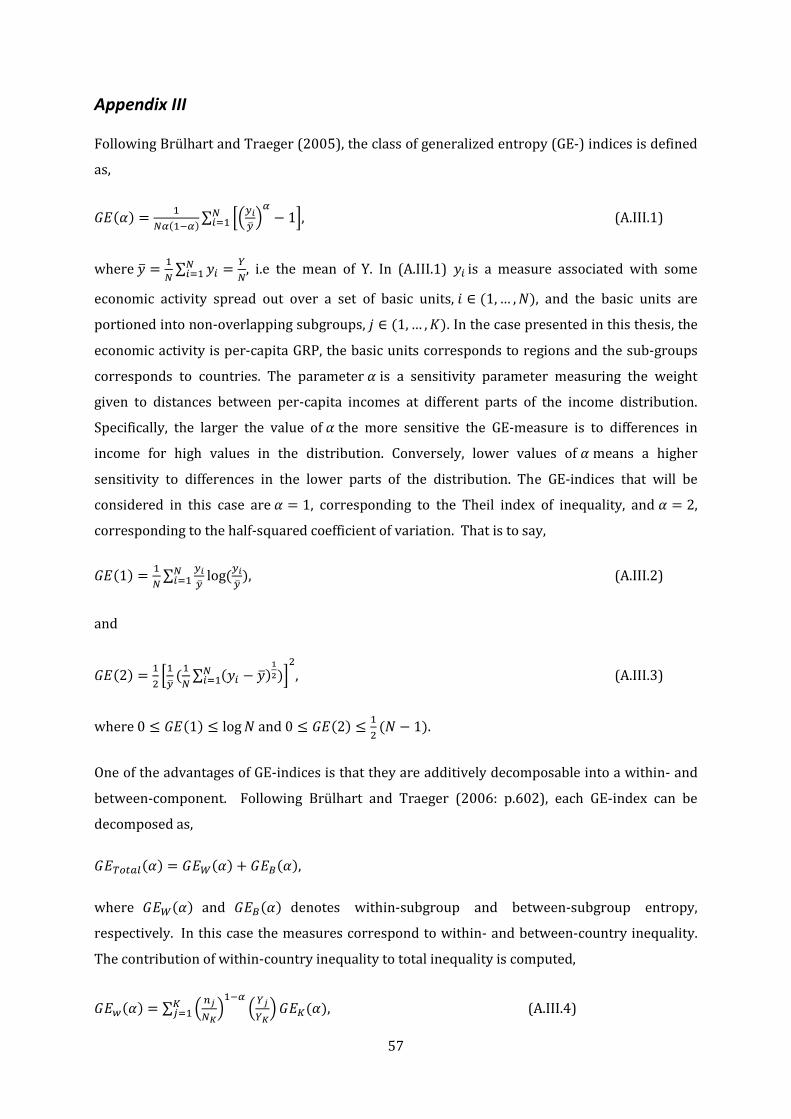
57
Appendix III
Following Brülhart and Traeger (2005), the class of generalized entropy (GE-) indices is defined
as,
∑ [(
) ]
, (A.III.1)
where
∑
, i.e the mean of Y. In (A.III.1) is a measure associated with some
economic activity spread out over a set of basic units, , and the basic units are
portioned into non-overlapping subgroups, . In the case presented in this thesis, the
economic activity is per-capita GRP, the basic units corresponds to regions and the sub-groups
corresponds to countries. The parameter is a sensitivity parameter measuring the weight
given to distances between per-capita incomes at different parts of the income distribution.
Specifically, the larger the value of the more sensitive the GE-measure is to differences in
income for high values in the distribution. Conversely, lower values of means a higher
sensitivity to differences in the lower parts of the distribution. The GE-indices that will be
considered in this case are , corresponding to the Theil index of inequality, and ,
corresponding to the half-squared coefficient of variation. That is to say,
∑
, (A.III.2)
and
[
∑
]
, (A.III.3)
where and
.
One of the advantages of GE-indices is that they are additively decomposable into a within- and
between-component. Following Brülhart and Traeger (2006: p.602), each GE-index can be
decomposed as,
,
where and denotes within-subgroup and between-subgroup entropy,
respectively. In this case the measures correspond to within- and between-country inequality.
The contribution of within-country inequality to total inequality is computed,
∑ (
)
(
)
(A.III.4)
58
where is the GE-index as defined by (A.III.1) but only for regions i belonging to country j,
so that N becomes . Thus, within-country GE-indices are calculates as if each country is its own
population. Subsequently, the contribution of between-country inequality is calculated by
applying (A.III.1) to country j’s mean, , instead of the mean of the entire population, .
Generally, -indices are preferred for decomposition (ibid). This comes from that
decompositions of weights are based on both shares and shares, meaning that the
weights of are not independent from the weights of . The consequence of this
being that the within- and between-component of the -weights need not be scale invariant
or sum to a one.
Appendix IV
Following Silverman (1986), a kernel density estimator is a non-parametric technique to derive
the probability density distribution of a random variable. The method tries to fit an unknown
distribution of the random variable to a priori chosen distribution. The kernel density estimator
takes the following form,
∑ (
)
, (A.IV.1)
Where in this case is the per-capita GRP of region i at time t, is the average per-capita
income over the whole sample at time t, is the smoothing parameter and is a kernel
function. The kernel function defines the distributional function that the data is to be fitted to
and can take many forms with the only requisite that it is symmetric and integrates to one.
There is no real criterion for choosing optimal kernel function or bandwidth. However, following
the literature on regional income disparities a Gaussian kernel function is chosen. That is, it is
assumed that the distribution of the unknown variable (the regional per-capita income
distribution in this case) follows the standard-normal Gaussian distribution. Following Fox
(1990), given a Gaussian kernel function, the smoothing parameter, , also known as the
bandwidth, is chosen so that the mean integrated squared error of the assumed distribution is
minimized for each observation in every time period. If the true distribution of regional per-
capita incomes do not differ markedly from the normal distribution this method should yield an
efficient estimate (Geppert and Stephen 2008: p.195).