an empirical evaluation of mutation and crossover

Simula Research Laboratory, Technical Report, 2017-02 Jan, 2017

An Empirical Evaluation of Mutation and Crossover

Operators for Multi-Objective Uncertainty-Wise Test

Minimization

Shaukat Ali1, Yan Li1, Tao Yue1,2, Man Zhang1

(The authors are alphabetically ordered) 1Simula Research Laboratory, Norway

2The University of Oslo, Norway

{shaukat, adeng, tao, manzhang}@simula.no

Abstract—Multi-objective uncertainty-wise test case

minimization focuses on selecting a minimum number of test

cases to execute out of all available ones while maximizing

effectiveness (e.g., coverage), minimizing cost (e.g., time to

execute test cases), and at the same time optimizing uncertainty-

related objectives. In our previous unpublished work1, we

developed four uncertainty-wise test case minimization strategies

relying on Uncertainty Theory and multi-objective search

(NSGA-II with default settings), which were evaluated with one

real Cyber-Physical System (CPS) with inherent uncertainty.

However, a fundamental question to answer is whether these

default settings of NSGA-II are good enough to provide

optimized solutions. In this direction, we report one of the

preliminary empirical evaluations, where we performed an

experiment with three different mutation operators and three

crossover operators, i.e., in total nine combinations with NSGA-

II for the four uncertainty-wise test case minimization strategies

using a real CPS case study. Results show that the Blend Alpha

crossover operator together with the polynomial mutation

operator permits NSGA-II achieving the best performance for

solving our uncertainty-wise test minimization problems.

Keywords—Uncertainty-Wise Testing; Test Case Minimization;

Multi-objective Search; Cyber-Physical Systems

I. INTRODUCTION

The internal behavior of a Cyber-Physical System (CPS)

under Test (CUT) is typically known to a limited extent [1-3].

In addition, a CPS interacts with the physical environment

including agents (e.g., human), which is fundamentally

indeterminate [1-3]. This means that uncertainty regarding the

internal behavior of a CUT must be explicitly taken into the

account together with uncertainty in its environment when

performing any kind of testing. Traditional testing methods for

CPS [4-6] do not handle uncertainty explicitly and thus novel

testing approaches for CPS must be made “uncertainty-wise”.

In the direction of making testing techniques “uncertainty-

wise”, we proposed an uncertainty testing framework called

UncerTest in our previous unpublished work 1 [7]. The

UncerTest framework defines a set of uncertainty-wise test

case generation and minimization strategies for CPSs. The key

1 This is an unpublished work (reference number [7]) reported in a project

deliverable and made available as a technical report.

inputs for UncerTest are tested ready models of a CUT with

explicitly modeled subjective uncertainty on its internal

behavior and test ready models of the physical environment

with uncertainty. Such test ready models (extended UML class

diagram, state machines, and object diagrams) were developed

with our uncertainty modeling framework called UncerTum

presented in [8]. Uncertainty-wise test case minimization

strategies in UncerTest were designed and implemented based

on Uncertainty Theory [9] and multi-objective search (NSGA-

II [10] with default settings) and were evaluated with a real

CPS in terms of their cost, effectiveness, and efficiency.

Uncertainty-wise test case minimization strategies take into

consideration cost and effectiveness measures, including a

number of test cases to execute (cost), high coverage (transition

coverage), and at the same time focused on optimizing

uncertainty-related objectives [7]. These uncertainty related

objectives are a number of uncertainties in a test case, the

number of unique uncertainties in a test case, uncertainty space

coverage and uncertainty measure of a test case defined with

the uncertainty theory [9].

Our initial evaluation of the above mentioned uncertainty-

wise test case minimization strategies [7] only experimented

with default settings of NSGA-II implemented in jMetal [11].

A fundamental question to answer is whether these default

settings of NSGA-II are good enough for uncertainty-wise test

case minimization strategies. To this end, we report a

preliminary empirical evaluation, where we compared nine

combinations of mutation and crossover operators (three

crossover and three mutation operators) with NSGA-II, using a

CPS case study for the four uncertainty-wise test case

minimization strategies reported in [7]. The case study is a real

CPS about GeoSports provided to us by Future Position X,

Sweden (FPX)2 as part of our on-going project [12] with FPX

as an industrial partner.

Results of our empirical evaluation show that the Blend

Alpha crossover (BLX-) operator together with the

polynomial mutation operator can assist NSGA-II to attain the

best performance for our four uncertainty-wise test

2 www.fpx.se

mailto:manzhang%[email protected]


minimization problems, corresponding to the four uncertainty-

wise test strategies. Moreover, we observed that regardless of

the chosen mutation operator, the BLX- crossover operator

performs significantly better than the rest of the studied

crossover operators.

This paper is organized as follows: Section II presents the

background to understand the remaining sections of the paper.

Section III presents the planning of our empirical evaluation.

Section IV provides results and analyses. Section V presents

the related work and we conclude the paper in Section IV.

II. BACKGROUND

In a project deliverable1 [7], we presented UncerTest, an

uncertainty-wise test case generation, and minimization

framework. The input of UncerTest is test ready models

explicitly capturing uncertainty developed with UncerTum —

an uncertainty-wise test modeling framework 3 [8]. With

UncerTum test ready models are created with UML state

machines, UML class diagrams, and UML object diagrams.

Uncertainty information is added to various model elements

using the UML Uncertainty Profile (UUP) defined in

UncerTum. The UML state machines with applied UUP are

called Belief State Machines (BSMs). UncerTest then utilizes

two implemented test case generation strategies and four

minimization test strategies relying on the uncertainty theory

[9] and multi-objective search to generate executable test cases.

Such test cases are executed on a CPS to test its

implementation in the presence of uncertainty.

In UncerTest (reported in a project deliverable1) [7], we

defined four test case minimization problems that were solved

with multi-objective search. These problems with their

minimization objectives are listed in TABLE I.

TABLE I. UNCERTAINTY-WISE TEST CASE MINIMIZATION PROBLEMS [7]

P# ↓Objective 1 ↑ Objective 2 ↑ Objective 3

P1

% of test case

minimization

Average # of Uncertainties

covered

%Transition

coverage

P2 % Uncertainty Space

coverage P3 Average Uncertainty Measure

P4 % Unique Uncertainties

covered

Each test case has the following associated attributes: 1)

number of subjective uncertainties covered (Objective 2 for

P1), 2) uncertainty space covered as defined in the uncertainty

theory (Objective 2 for P2), 3) overall uncertainty of a test case

calculated using the uncertainty measure defined in the

uncertainty theory (Objective 2 for P3), 3) number of unique

uncertainties covered (Objective 2 for P4), and 4) number of

transitions covered (Objective 3 for P1--P4).

A test case minimization solution consists of a subset

(Tmsub) of a total number of test cases (Ttotal). Ttotal is generated

3 Notice that [8] is a technical report (under review of Sosym journal)

reporting a project deliverable.

from a BSM, i.e., a test ready model using a test case

generation strategy implemented in UncerTest.

Objective 1 is calculated as: 𝑂1 =𝑇𝑚𝑠𝑢𝑏

𝑇𝑡𝑜𝑡𝑎𝑙× 100%.

Objective 2 for P1 (i.e., Average # of Uncertainties

covered) is calculated as follows:

𝑂2𝑃1 =∑ 𝑛𝑜𝑟(𝑁𝑈(𝑡𝑖

′))𝑁𝑇msub𝑖=1

𝑁𝑇msub

In the above formula, 𝑁𝑇msub is the number of test cases in

the minimized subset. NU represents the number of

uncertainties in a test case and 𝑛𝑜𝑟(𝑁𝑈(𝑡𝑖′)) =

𝑁𝑈(𝑡𝑖′)

𝑁𝑈(𝑡𝑖′) +1

[13].

Objective 2 for P2 (i.e., % Uncertainty Space coverage) is

calculated as follows:

𝑂2𝑃2 =𝑚𝑢𝑠𝑝

𝑛𝑢𝑠𝑝× 100%

In the above formula, nusp represents the uncertainty space

covered [9] by a BSM from which the test cases are generated,

whereas musp represents the uncertainty space of Tmsub.

Objective 2 for P3 (i.e., Average Uncertainty Measure) is


𝑂2𝑃3 =∑ 𝑈𝑀(𝑡𝑖)

𝑁𝑇msub𝑖=1

𝑁𝑇msub

In the above formula, 𝑁𝑇msub is the number of test cases in

the minimized subset. UM(tx) represents the uncertainty

measure of a test case x using the uncertainty theory [9].

Objective 2 for P4 (i.e., Unique Uncertainties Covered) is


𝑂2𝑃4 =𝑚𝑢𝑢

𝑛𝑢𝑢× 100%

In the above formula, muu is the number of unique (non-

duplicate) uncertainties covered by Tmsub, whereas nuu is the

total number of uncertainties in a BSM.

Objective 3 is calculated as: 𝑂3 =𝑚𝑡𝑟

𝑛𝑡𝑟× 100%.

In the above formula, mtr is the number of unique

transitions covered by Tmsub, whereas ntr is the total number of

transitions in the BSM.

In the project deliverable (unpublished work) [7], we used

NSGA-II, the commonly used multi-objective search algorithm

to solve these four test case minimization problems. We used

the NSGA-II algorithm implemented in jMetal [11] with the

default parameter settings.

III. EMPIRICAL EVALUATION PLANNING

In this section, we will present our overall objective and

research questions (Section A), selection of the case study, the

algorithm, and operators (Section B), and design of our

experiment in Section C.


A. Overall Objective and Research Questions

Our overall objective is to study the impact of various

mutation and crossover operators for NSGA-II on the

effectiveness of the four uncertainty-wise test case

minimization techniques described in Section II and were

originally proposed in [7]. Based on our overall objective, we

defined the following research questions:

RQ1: For each uncertainty-wise test case minimization

strategy (P1 to P4 in Section II), how does NSGA-II compare

with the Random Search (RS), with each combination of the

mutation and crossover operator?

RQ2: Which combination of the mutation and crossover

operator helps an uncertainty-wise test case minimization

strategy (P1 to P4 in Section II) in achieving the best

performance?

RQ3: How do the interactions among the crossover and

mutation operators affect the performance of uncertainty-wise

test case minimization strategies?

The first research question helps us in assessing whether

the problems we are solving are complex and deserve the use

of a complex multi-objective search algorithm. Notice that this

is according to the commonly used guidelines for applying

search-based algorithms in software engineering [14]. The

second research question helps us in determining one or more

best combinations of the mutation and crossover operators that

we can recommend to use with each uncertainty-wise test case

minimization strategy. The third research question helps us in

studying the interactions among crossover and mutation

operators on the performance of NSGA-II.

B. Selection of Case Studies, Algorithm, and Operators

In this section, we present the two case studies that we

selected for our empirical evaluation, in addition to the

selection of the mutation and crossover operators.

1) Case Study

The case study is provided by Future Position X (FPX),

Sweden2—one of the industrial partners in our on-going project

[12]. The case study is an instance of GeoSports for Bandy (a

type of ice hockey). The CPS involves attaching various

sensors to collect health and bandy related measurements

including heartbeat, speed, and location. The collected

measurements are then transferred at runtime via a receiver

station (a Bluetooth-based antenna) to a computer system,

where those measurements can be monitored by Bandy

coaches. To facilitate automated execution of tests on such

CPS without real players, Nordic Med Test (NMT)4—another

partner provides test execution infrastructure. Given that the

physical infrastructure is used for execution of tests,

maximizing the effectiveness of test case execution with a

minimum number of test cases is of utmost importance due to

the fact that it is expensive both in terms of time to set up,

execute, and maintain it.

For the Bandy case study, we used UncerTum [8] to create

test ready models as reported in [7] and UncerTest with All

Path with Maximum Length (APML) was used to generate test

cases [7]. In total, for Bandy, 2085 test cases were generated.

These test cases were the input for our uncertainty-wise test

case minimization. Notice that for each test case, a number of

uncertainties, uncertainty space coverage, uncertainty measure,

and the number of unique uncertainties were calculated

automatically. Notice that in Section II, we briefly explained

these attributes; however further details can be consulted in [7].

2) NSGA-II Settings and Operators

We selected three mutation operators and three crossover

operators for NSGA-II—the most commonly used algorithm

for multi-objective optimization. The crossover operators

include Simulated Binary Crossover (SBX), Single Point

Crossover (SPX), and Blend Alpha Crossover (BLX-) [15].

The mutation operators include Polynomial (M1), Non-

Uniform (M2), and Swap (M3). Thus, we had nine

combinations of the mutation and crossover operators (CM1 to

CM9).

Given that random variation is inherent in search

algorithms, we ran NSGA-II and RS 100 times each to deal

with the random variation. We used the jMetal framework [11]

for the implementation of both NSGA-II and RS. The

population size was set to 100, the binary tournament was used

for the selection parents, and the simulated binary criterion was

used for recombination. Notice that as an initial empirical

evaluation, we only evaluated the combination of the mutation

and crossover operators and kept the rest of the settings default.

C. Experiment Design

The design of our experiment is shown in TABLE II. As

shown in the table, for each uncertainty-wise test case

minimization problem (P1--P4) as described in Section II, we

used the Bandy case study to answer the three research

questions defined in Section A.

For RQ1 as shown in TABLE II, we compared NSGA-II

together with each combination of the crossover and mutation

4 www.nordicmedtest.se/

TABLE II. DESIGN OF THE EXPERIMENT*

Problem Case Study RQ Comparison Metrics Statistical Methods

P1--P4 Bandy 1 NSGA-II (CM1-CM9) vs RS

HV, O1, O2P1 (only for P1), O2P2 (only for P2), O2P3 (only for P3), O2P4 (only for P4),

O3, OFVP1, OFVP2, OFVP3

𝐴12̂, 𝑝 –value (Mann-Whitney U Test)

2 NSGA-II (CMi) vs NSGA-II (CMj) and i≠j, i= 1..9, j=1..9

𝐴12̂, p-value (Kruskal–Wallis test with Bonferroni Correction), p-value (Mann-

Whitney U Test)

3 Interactions of Crossover and

Mutation Operators on response variables (i.e., metrics)

Two-Way Analysis of Variance (ANOVA)

*CM1=SBX with M1, CM2: SBX with M2, CM3: SBX with M3, CM4: SPX with M1, CM5: SPX with M2, CM6: SPX with M3, CM7: BLX-α with M1, CM8: BLX- α with M2, CM9: BLX- α with M3


operators (CM1 to CM9) with RS, i.e., in total 9 comparisons.

For RQ2, we compared NSGA-II with each pair of the

combinations of the crossover and mutation operators, for

example, NSGA-II (with CM1) with NSGA-II (with CM2) and

so on. In total, we have 9C2 pairs of comparisons. For RQ3, we

performed interaction analysis of the crossover and mutation

operators on the performance of NSGA-II.

As shown in the Metrics column of TABLE II, for each

pair of comparison, we used a set of metrics. First, we used

HyperVolume (HV) [16] as the quality indicator, which was

selected based on the guidelines of selecting an appropriate

quality indicator for search-based software engineering (SBSE)

problems [17]. Second, we also performed the comparison

using the individual objectives relevant for each problem, i.e.,

O1, O2P1, O3 for P1, O1, O2P2, O3 for P2, O1, O2P3, O3 for P3,

and O1, O2P4, O3 for P4. Notice that in each run of NSGA-II, it

produces a set of non-dominated solutions (100 in our case)

constituting a Pareto front. For each individual objective (e.g.,

O1), we select the best solution with the highest value of the

objective function (e.g., O1) for comparison out of all the 100

non-dominated solutions produced by NSGA-II in this run.

Third, we also performed the comparison using Overall Fitness

Value (OFV) for each problem (P1--P4). OFVP1 is calculated

as (O1+O2P1+O3)/3, OFVP2 is calculated as (O1+O2P2+O3)/3,

OFVP3 is calculated as (O1+O2P3+O3)/3, and OFVP4 is

calculated as (O1+O2P4+O3)/3. For each run, we calculate

OFV for each of the 100 non-dominated solutions for each run.

In this way, we have 100*100 (10,000) OFV values to compare

for 100 runs.

In terms of statistical methods, for each pair of comparison,

we used 𝐴12̂ as an effect size measure, whereas the Mann-Whitney U Test was used to assess the statistical significance of results. These two tests were chosen based on the guidelines of reporting results of SBSE [14]. For RQ2, since we have (9C2), i.e., 36 pair-wise comparisons, we first used the Kruskal–Wallis test with Bonferroni Correction to determine if overall statistically significant differences exist among all the pairs

together. For both the Mann-Whitney and Kruskal–Wallis, we chose the significance level of 0.05, i.e., a value less than 0.05 shows statistically significant differences. In case of significant differences, pair-wise comparisons were performed with the

Mann-Whitney U Test. In terms of 𝐴12̂, a value of 0.5 means no difference between a pair being compared, a value less than 0.05 means that the first in the pair has higher chance to get a better solution than the second one, whereas a value greater than 0.5 means vice versa. For RQ3, we chose the Two-Way Analysis of Variance (ANOVA) to study the interactions among the crossover and mutation operators on objective values and HV [18, 19].

IV. RESULTS AND ANALYSIS

In this section, we present our results and analyses

corresponding to the research questions.

A. Results for RQ1

All the detailed results are provided in Appendix A. For P1

in terms of O1, O2P1, OFVP1, and HV, NSGA-II performed

significantly better than RS. For O3, either there were no

significant differences between NSGA-II and RS or RS was

significantly better than NSGA-II. Recall that O3 is about the

All Transition coverage and thus RS always selected more test

cases (i.e., less percentage of test minimization) and thus

covered more transitions than NSGA-II. For P2, P3, and P4,

we observed the similar pattern as P1, except that for O3, we

didn’t observe any difference between NSGA-II and RS.

Based on the results, we can conclude that regardless of the

combination of the mutation and crossover operators, NSGA-II

managed to significantly outperform RS in terms of HV and

OFV, suggesting that our problems are difficult to solve and

require the use of multi-objective search algorithms.

B. Results for RQ2

To answer RQ2, for each problem (P1--P4), first, we

compared overall differences among (9C2), i.e., 36

combinations all together using the Kruskal–Wallis test with

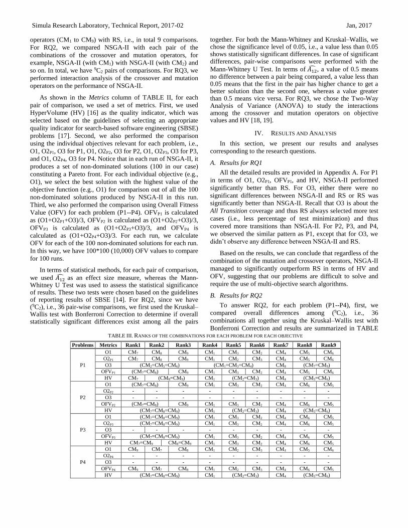
Bonferroni Correction and results are summarized in TABLE TABLE III. RANKS OF THE COMBINATIONS FOR EACH PROBLEM FOR EACH OBJECTIVE

Problems Metrics Rank1 Rank2 Rank3 Rank4 Rank5 Rank6 Rank7 Rank8 Rank9

P1

O1 CM7 CM8 CM9 CM1 CM3 CM2 CM4 CM5 CM6

O2P1 CM7 CM8 CM9 CM1 CM2 CM3 CM4 CM5 CM6

O3 (CM2=CM5=CM6) (CM1=CM3=CM4) CM8 (CM7=CM9)

OFVP1 (CM7=CM8) CM9 CM1 CM3 CM2 CM4 CM5 CM6

HV CM7 (CM8=CM9) CM1 (CM2=CM3) CM4 (CM5=CM6)

P2

O1 (CM7=CM8) CM9 CM1 CM3 CM2 CM4 CM6 CM5

O2P2 - - - - - - - - -

O3 - - - - - - - - -

OFVP2 (CM7=CM8) CM9 CM1 CM3 CM2 CM4 CM6 CM5

HV (CM7=CM8=CM9) CM1 (CM2=CM3) CM4 (CM5=CM6)

P3

O1 (CM7=CM8=CM9) CM1 CM3 CM2 CM4 CM6 CM5

O2P3 (CM7=CM8=CM9) CM1 CM3 CM2 CM4 CM6 CM5

O3 - - - - - - - - -

OFVP3 (CM7=CM8=CM9) CM1 CM3 CM2 CM4 CM6 CM5

HV CM7=CM9 CM8=CM9 CM1 CM3 CM2 CM4 CM6 CM5

P4

O1 CM9 CM7 CM8 CM1 CM2 CM3 CM4 CM5 CM6

O2P4 - - - - - - - - -

O3 - - - - - - - - -

OFVP4 CM9 CM7 CM8 CM1 CM2 CM3 CM4 CM6 CM5

HV (CM7=CM8=CM9) CM1 (CM2=CM3) CM4 (CM5=CM6)


IV. Notice that most of the time, p-values are less than 0.0001

suggesting that significant differences exist among pairs in

terms of the individual objectives, OFV, and HV. For the cells

with a “-“ value means no significant differences. We further

compared each pair of crossover and mutation operator using

the Mann-Whitney U Test and 𝐴12, only for the cases when the

Kruskal–Wallis test revealed significant differences. Due to the

large number of comparisons and lack of space in this paper,

we only report summarized results in TABLE IV. However,

the detailed results including p-values and 𝐴12 are reported in

Appendix B.

TABLE IV. RESULTS OF THE KRUSKAL–WALLIS TEST

Problems O1 O2Pi for Pi O3 OFVPi for Pi HV

P1 <.0001 <.0001 <.0001 <.0001 <.0001

P2 <.0001 - - <.0001 <.0001

P3 <.0001 <.0001 - <.0001 <.0001

P4 <.0001 - - <.0001 <.0001

In TABLE III, a “-” means that we did not perform a pair-

wise comparison since we did not observe overall differences

using the Kruskal–Wallis test (e.g., O2P2 and O3 for P2). For

P1, except for O3, CM7 is the best combination. For P2, CM7

and CM8 are the best combinations for O1 and OFVP2 and for

HV CM7 to CM9. For P3, O1, O2P3, OFVP3, CM7 to CM9 are

the best combinations, whereas for HV both CM7 and CM9 are

the best ones. For P4, when looking at O1 and OFVP1, CM9 is

the best, whereas for HV CM7 to CM9 are the best

combinations.

Across all the problems, when we consider HV—the most

commonly used quality indicator used to assess the quality of

solutions produced by Pareto optimality based algorithms [16,

17], we have a clear winner, i.e., CM7. The CM7 is the

combination of the BLX- crossover operator with the

polynomial mutation operator.

C. Results for RQ3

For each problem, we additionally performed Two-Way

ANOVA to study the significance of the interactions among

the crossover and mutation operators on the objectives and HV.

The detailed results with exact p-values are provided in

Appendix C. We only provide interaction plots for all the four

problems, only for those objectives/HV when the interactions

had a significant impact on objectives/HV. For example, for

P1, there were no significant interactions for O2P1 and O3 and

for the rest, the results were significant (p<0.05) and thus we

do not show plots for O2P1 and O3. In Figure 1 for P1, in terms

of O1/O2P1/OFVP1, C1 and C3 give the best results with M1

and M2 (lower values), whereas when considering mutation

operators (M1-M3), C3 has the best performance with all the

(P1-O1)

(P1-O2P2)

(P1-O3)

(P1-OFVP1)

(P1-HV)

(P2-O1)

(P2-OFVP2)

(P2-HV)

(P3-O1)

(P3-O2P3)

(P3-OFVP3)

(P3-HV)

(P4-O1)

(P4-OFVP4)

(P4-HV)

Figure 1. Interaction Plots of Problem 1 (P1), Problem 2 (P2), Problem 3 (P3) and Problem 4 (P4)


mutation operators followed by C1 and C2. For HV (notice that

higher values mean better performance), the results are also

consistent. For P2/P4, the observed results are exactly the same

as P1. For P3, results are the same as well except that we had

additional results for O2P3, which are also consistent with the

rest of the objectives.

Based on the above results, we can conclude that the C3

crossover mutation operator with any mutation operator

consistently gives the best results for all the four uncertainty-

wise test minimization problems.

D. Overall Discussion

Based on the results and discussions in the previous sections,

we recommend using CM7 together with NSGA-II with default

parameter settings to solve our uncertainty-wise test case

minimization problems. Since CM7 (equal to CM8 or equal to

CM9) turns out to be the winner, when considering HV, i.e., the

most commonly used quality indicator to assess the quality of

the solutions produced by multi-objective search algorithms

based on the Pareto optimality theory.

When further analyzing CM7 to CM9, we can see that all

the three combinations use the same crossover operator, i.e.,

BLX- and it gives us an indication that this crossover

operator plays a significant role on the performance of NSGA-

II for our uncertainty-wise test case minimization problems.

This was further confirmed with the interactions analyses

reported in Section C, where C3 (i.e., the BLX- operator)

with any combination of the mutation operator was the best

one for all the four problems (Figure 1).

Evidence has shown that BLX- has a good capability of

exploring a search space [20, 21], as compared to, for example,

SBX and SPX. One probable explanation is that in our context,

NSGA-II needed to explore more search space (in a given

number of generations) as compared to exploiting the nearby

search space of parents, to find the most optimized solutions.

However, this explanation needs to be further justified with

further experimentation and theoretical analysis that we plan to

conduct in the near future.

E. Threats to Validity

All the experiments have their associated threats to validity.

In terms of internal validity, we used default parameter settings

of NSGA-II except for the combinations of crossover and

mutation operators. However, these default values were chosen

based on the guidelines reported in [14, 22, 23]. Additionally,

in this preliminary experiment, we only chose three crossover

and three mutation operators, and several other such operators

exist that can be used. We chose these operators since their

implementation was readily available in jMetal. We plan to

conduct more experiments in the near future to include more

crossover and mutation operators. In terms of external validity

threats, we only used one industrial case study and no doubt,

additional experiments with different case studies are necessary

to generalize the results.

For conclusion validity related to the randomness of

solutions produced by search algorithms [24], we repeated the

experiments 100 times [24] according to standard guidelines

[14]. Following the same guidelines, we used the appropriate

statistical tests, e.g., the Vargha and Delaney statistics to

calculate effect size, and the Mann-Whitney U test to

determine the significance of results. Construct validity threats

are concerned with the use of measures for comparing

performance [24]. We used the same stopping criterion (25000

fitness evaluations [24]) for all NSGA-II and RS to avoid any

potential bias in results.

V. RELATED WORK

A detailed survey on SBSE is reported in [25]. The survey

reports various types of software engineering problems that are

solved with SBSE in addition to reporting various trends of

search algorithms’ applications and techniques. Based on the

review, it is clear that test case minimization is one of the

widely addressed problems in SBSE. Other surveys reported in

[26] and [27], provide various test optimization objectives in

the context of regression testing, e.g., based on code coverage

and fault detection. In addition, even existing search-based test

optimization approaches are based on typical cost measures,

e.g., time to execute test cases and measure effectiveness, for

instance, using code coverage [28, 29] and fault detection [17,

30, 31]. Our uncertainty-wise test case minimization

objectives, i.e., the number of uncertainties, the number of

unique uncertainties, uncertainty space coverage, and

uncertainty measure are new. However, transition coverage has

been already been studied [27, 32].

Our uncertainty testing framework, named as UncerTest

was reported in the project deliverable1 [7], where we

originally proposed uncertainty-wise test case generation and

minimization approaches. However, in [7], we only

experimented with the default parameter settings and default

mutation and crossover operators of NSGA-II. In this work, we

experimented with combinations of the mutation and crossover

operators. Based on the results of our experiments, the

guidelines for selecting an appropriate combination of the

mutation and crossover operator are proposed. These

guidelines will be implemented in UncerTest.

In our another work reported in [33], we proposed an

uncertainty-wise time-aware test prioritization approach that

uses the same objectives as this one but focuses exclusively on

test prioritization rather than minimization as the project

deliverable reported in [7] and in this paper. In addition, the

key contribution of this paper is to empirically investigate

various combinations of the mutation and crossover operators

with NSGA-II with the ultimate aim of deriving a set of

guidelines to select an appropriate combination of the mutation

and crossover operators for our problems.

Existing search-based optimization approaches address

uncertainty in software project planning [34] and in the early

stage, e.g. requirement analysis [35-37] to enable the decision

making in uncertainty. In contrast, our works [7, 33] address

uncertainty in test optimization.


VI. CONCLUSION AND FUTURE WORK

This paper presented an empirical evaluation assessing the

effect of 9 combinations of 3 crossover and 3 mutation

operators on the performance of NSGA-II for four uncertainty-

wise test case minimization problems. We used test cases

generated for a real Cyber-Physical System (CPS) provided by

Future Position X related to GeoSports (for Bandy sports). The

results of the empirical evaluation show that the Blend Alpha

Crossover operator (BLX-) with the polynomial mutation

operator enables NSGA-II to achieve the best performance for

our uncertainty-wise test case minimization problems.

Furthermore, we concluded that for our problems, BLX- with

other evaluated mutation operators also gave good performance

suggesting that irrespective of a mutation operator, BLX- can

help NSGA-II achieve the best performance for our

uncertainty-wise test case minimization problems. In the

future, we would like to extensively extend our empirical

evaluation with additional mutation and crossover operators

and include other case studies for evaluation.

ACKNOWLEDGMENT

This research was supported by the EU Horizon 2020

funded project (Testing Cyber-Physical Systems under

Uncertainty). Tao Yue and Shaukat Ali are also supported by

RCN funded Zen-Configurator project, RFF Hovedstaden

funded MBE-CR project, RCN funded MBT4CPS project, and

RCN funded Certus SFI.

REFERENCES

[1] D. B. Rawat, J. J. Rodrigues, and I. Stojmenovic, Cyber-physical

systems: from theory to practice: CRC Press, 2015.

[2] S. Sunder, "Foundations for Innovation in Cyber-Physical Systems." [3] E. Geisberger, and M. Broy, Living in a networked world: Integrated

research agenda Cyber-Physical Systems (agendaCPS): Herbert Utz

Verlag, 2015. [4] N. Walkinshaw, and G. Fraser, “Uncertainty-Driven Black-Box Test

Data Generation,” arXiv preprint arXiv:1608.03181, 2016.

[5] R. Poli, W. B. Langdon, N. F. McPhee, and J. R. Koza, A field guide to genetic programming: Lulu. com, 2008.

[6] V. Garousi, "Traffic-aware stress testing of distributed real-time systems

based on UML models in the presence of time uncertainty." pp. 92-101. [7] M. Zhang, S. Ali, T. Yue, and M. Hedman, "Uncertainty-based Test

Case Generation and Minimization for Cyber-Physical Systems: A

Multi-Objective Search-based Approach", Technical report, Simula Research Laboartory, 2017, unpublished,

https://www.simula.no/publications/uncertainty-based-test-case-

generation-and-minimization-cyber-physical-systems-multi. [8] M. Zhang, S. Ali, T. Yue, and R. Norgre, "An Integrated Modeling

Framework to Facilitate Model-Based Testing of Cyber-Physical

Systems under Uncertainty", Technical report, Simula Research Laboartory, 2017, under review,

https://www.simula.no/publications/integrated-modeling-framework-

facilitate-model-based-testing-cyber-physical-systems. [9] B. Liu, Uncertainty theory: Springer, 2015.

[10] K. Deb, A. Pratap, S. Agarwal, and T. Meyarivan, “A fast and elitist

multiobjective genetic algorithm: NSGA-II,” IEEE transactions on evolutionary computation, vol. 6, no. 2, pp. 182-197, 2002.

[11] A. J. Nebro, and J. J. Durillo. "jMetal," 2016;

http://jmetal.sourceforge.net/. [12] S. Ali, and T. Yue, "U-Test: Evolving, Modelling and Testing Realistic

Uncertain Behaviours of Cyber-Physical Systems." 8th International

Conference on Software Testing, Verification and Validation (ICST). IEEE, 2015. pp. 1-2.

[13] A. Arcuri, “It really does matter how you normalize the branch distance

in search‐based software testing,” Software Testing, Verification and

Reliability, vol. 23, no. 2, pp. 119-147, 2013. [14] A. Arcuri, and L. Briand, "A practical guide for using statistical tests to

assess randomized algorithms in software engineering." 33rd

International Conference on Software Engineering (ICSE). IEEE, 2011. [15] J. Eshelman Larry, and J. Schaffer David, “Real-coded Genetic

Algorithms and Interval-Schemata,” Foundations of Genetic Algorithms,

vol. 2. [16] E. Zitzler, and L. Thiele, “Multiobjective evolutionary algorithms: a

comparative case study and the strength Pareto approach,” IEEE

transactions on Evolutionary Computation, vol. 3, no. 4, pp. 257-271, 1999.

[17] S. Wang, S. Ali, T. Yue, Y. Li, and M. Liaaen, "A practical guide to

select quality indicators for assessing pareto-based search algorithms in search-based software engineering.", Proc. of the 38th International

Conference on Software Engineering. ACM, 2016, pp. 631-642.

[18] Y. Fujikoshi, “Two-way ANOVA models with unbalanced data,” Discrete Mathematics, vol. 116, no. 1-3, pp. 315-334, 1993.

[19] L.-W. Xu, F.-Q. Yang, and S. Qin, “A parametric bootstrap approach for

two-way ANOVA in presence of possible interactions with unequal

variances,” Journal of Multivariate Analysis, vol. 115, pp. 172-180,

2013. [20] D. Ortiz-Boyer, C. Hervás-Martínez, and N. García-Pedrajas, “CIXL2:

A Crossover Operator for Evolutionary Algorithms Based on Population

Features,” J. Artif. Intell. Res.(JAIR), vol. 24, pp. 1-48, 2005. [21] F. Herrera, M. Lozano, and A. M. Sánchez, “A taxonomy for the

crossover operator for real‐coded genetic algorithms: An experimental

study,” International Journal of Intelligent Systems, vol. 18, no. 3, pp.

309-338, 2003. [22] D. J. Sheskin, Handbook of parametric and nonparametric statistical

procedures: crc Press, 2003.

[23] M. Harman, P. McMinn, J. T. De Souza, and S. Yoo, "Search based software engineering: Techniques, taxonomy, tutorial," Empirical

software engineering and verification, pp. 1-59: Springer, 2012.

[24] S. Wang, S. Ali, and A. Gotlieb, "Minimizing test suites in software product lines using weight-based genetic algorithms." Proc. of the 15th

annual conference on Genetic and evolutionary computation. ACM,

2013. pp. 1493-1500.

[25] M. Harman, S. A. Mansouri, and Y. Zhang, “Search-based software

engineering: Trends, techniques and applications,” ACM Comput. Surv.,

vol. 45, no. 1, 2012, pp. 1-61. [26] M. Harman, "Making the Case for MORTO: Multi Objective Regression

Test Optimization." 4th International Conference on Software Testing,

Verification and Validation Workshops (ICSTW), IEEE. 2011. [27] S. Yoo, and M. Harman, “Regression testing minimization, selection and

prioritization: a survey,” Softw. Test. Verif. Reliab., vol. 22, no. 2, pp.

67-120, 2012. [28] K. R. Walcott, M. L. Soffa, G. M. Kapfhammer, and R. S. Roos,

“TimeAware test suite prioritization,” in Proceedings of the 2006

international symposium on Software testing and analysis, Portland, Maine, USA, 2006, pp. 1-12.

[29] C. Henard, M. Papadakis, G. Perrouin, J. Klein, and Y. L. Traon, "Multi-

objective test generation for software product lines." Proc. of the 17th International Software Product Line Conference. ACM, 2013.pp. 62-71.

[30] L. Zhang, S.-S. Hou, C. Guo, T. Xie, and H. Mei, "Time-aware test-case

prioritization using integer linear programming." Proce. of the 8th

international symposium on Software testing and analysis. ACM, 2009.

[31] S. Wang, S. Ali, and A. Gotlieb, “Cost-effective test suite minimization

in product lines using search techniques,” Journal of Systems and Software, vol. 103, pp. 370-391, 2015.

[32] D. Xu, and J. Ding, "Prioritizing State-Based Aspect Tests." 3rd

International Conference on Software Testing, Verification and Validation (ICST). IEEE, 2010, pp. 265-274.

[33] S. Ali, Y. Li, T. Yue, and M. Zhang, "Uncertainty-Wise and Time-

Aware Test Case Prioritization with Multi-Objective Search", Technical report, Simula Research Laboartory, 2017, under review,

https://www.simula.no/publications/uncertainty-wise-and-time-aware-

test-case-prioritization-multi-objective-search. [34] F. Sarro, A. Petrozziello, and M. Harman, “Multi-objective software

effort estimation,” in Proceedings of the 38th International Conference on Software Engineering, Austin, Texas, 2016, pp. 619-630.

https://www.simula.no/publications/uncertainty-based-test-case-generation-and-minimization-cyber-physical-systems-multi

https://www.simula.no/publications/uncertainty-based-test-case-generation-and-minimization-cyber-physical-systems-multi

https://www.simula.no/publications/integrated-modeling-framework-facilitate-model-based-testing-cyber-physical-systems

https://www.simula.no/publications/integrated-modeling-framework-facilitate-model-based-testing-cyber-physical-systems

http://jmetal.sourceforge.net/

https://www.simula.no/publications/uncertainty-wise-and-time-aware-test-case-prioritization-multi-objective-search

https://www.simula.no/publications/uncertainty-wise-and-time-aware-test-case-prioritization-multi-objective-search


[35] L. Li, M. Harman, E. Letier, and Y. Zhang, “Robust next release

problem: handling uncertainty during optimization,” in Proceedings of

the 2014 Annual Conference on Genetic and Evolutionary Computation,

Vancouver, BC, Canada, 2014, pp. 1247-1254.

[36] S. Gueorguiev, M. Harman, and G. Antoniol, “Software project planning for robustness and completion time in the presence of uncertainty using

multi objective search based software engineering,” in Proceedings of

the 11th Annual conference on Genetic and evolutionary computation, Montreal, Québec, Canada, 2009, pp. 1673-1680.

[37] L. Li, M. Harman, F. Wu, and Y. Zhang, “The Value of Exact Analysis

in Requirements Selection,” IEEE Transactions on Software Engineering, vol. PP, no. 99, pp. 1-1, 2016.


Appendix A. Statistic Analysis Result for RQ1

Table A 1. Mann-Whitney U Test between NSGA-II (CM1-CM9) VS RS For P1 with Bandy

CM

Metrics

Prob O1 O2Pi for Pi O3 OFVPi for Pi HV

P1

CM1 �̂�12<0.1, p<0.05 �̂�12<0.1, p<0.05 �̂�12>0.5, p<0.05 �̂�12<0.1, p<0.05 �̂�12>0.9, p<0.05

CM2 �̂�12<0.1, p<0.05 �̂�12<0.1, p<0.05 �̂�12=0.5,p=1.0 �̂�12<0.1, p<0.05 �̂�12>0.9, p<0.05

CM3 �̂�12<0.1, p<0.05 �̂�12<0.1, p<0.05 �̂�12>0.5, p<0.05 �̂�12<0.1, p<0.05 �̂�12>0.9, p<0.05

CM4 �̂�12<0.1, p<0.05 �̂�12<0.1, p<0.05 �̂�12=0.5, p=1.0 �̂�12<0.1, p<0.05 �̂�12>0.9, p<0.05

CM5 �̂�12<0.1, p<0.05 �̂�12<0.1, p<0.05 �̂�12=0.5,p=1.0 �̂�12<0.1, p<0.05 �̂�12>0.9, p<0.05

CM6 �̂�12<0.1, p<0.05 �̂�12<0.1, p<0.05 �̂�12=0.5,p=1.0 �̂�12<0.1, p<0.05 �̂�12>0.9, p<0.05

CM7 �̂�12<0.1, p<0.05 �̂�12<0.1, p<0.05 �̂�12>0.5, p<0.05 �̂�12<0.1, p<0.05 �̂�12>0.9, p<0.05

CM8 �̂�12<0.1, p<0.05 �̂�12<0.1, p<0.05 �̂�12>0.5, p<0.05 �̂�12<0.1, p<0.05 �̂�12>0.9, p<0.05

CM9 �̂�12<0.1, p<0.05 �̂�12<0.1, p<0.05 �̂�12>0.5, p<0.05 �̂�12<0.1, p<0.05 �̂�12>0.9, p<0.05

P2

CM1 �̂�12<0.1, p<0.05 �̂�12=0.5, p=1.0 �̂�12=0.5, p=1.0 �̂�12<0.1, p<0.05 �̂�12>0.9, p<0.05

CM2 �̂�12<0.1, p<0.05 �̂�12=0.5, p=1.0 �̂�12=0.5, p=1.0 �̂�12<0.1, p<0.05 �̂�12>0.9, p<0.05

CM3 �̂�12<0.1, p<0.05 �̂�12=0.5, p=1.0 �̂�12=0.5, p=1.0 �̂�12<0.1, p<0.05 �̂�12>0.9, p<0.05

CM4 �̂�12<0.1, p<0.05 �̂�12=0.5, p=1.0 �̂�12=0.5, p=1.0 �̂�12<0.1, p<0.05 �̂�12>0.9, p<0.05

CM5 �̂�12<0.1, p<0.05 �̂�12=0.5, p=1.0 �̂�12=0.5, p=1.0 �̂�12<0.1, p<0.05 �̂�12>0.9, p<0.05

CM6 �̂�12<0.1, p<0.05 �̂�12=0.5, p=1.0 �̂�12=0.5, p=1.0 �̂�12<0.1, p<0.05 �̂�12>0.9, p<0.05

CM7 �̂�12<0.1, p<0.05 �̂�12=0.5, p=1.0 �̂�12=0.5, p=1.0 �̂�12<0.1, p<0.05 �̂�12>0.9, p<0.05

CM8 �̂�12<0.1, p<0.05 �̂�12=0.5, p=1.0 �̂�12=0.5, p=1.0 �̂�12<0.1, p<0.05 �̂�12>0.9, p<0.05

CM9 �̂�12<0.1, p<0.05 �̂�12=0.5, p=1.0 �̂�12=0.5, p=1.0 �̂�12<0.1, p<0.05 �̂�12>0.9, p<0.05

P3

CM1 �̂�12<0.1, p<0.05 �̂�12<0.1, p<0.05 �̂�12=0.5, p=1.0 �̂�12<0.1, p<0.05 �̂�12>0.9, p<0.05

CM2 �̂�12<0.1, p<0.05 �̂�12<0.1, p<0.05 �̂�12=0.5, p=1.0 �̂�12<0.1, p<0.05 �̂�12>0.9, p<0.05

CM3 �̂�12<0.1, p<0.05 �̂�12<0.1, p<0.05 �̂�12=0.5, p=1.0 �̂�12<0.1, p<0.05 �̂�12>0.9, p<0.05

CM4 �̂�12<0.1, p<0.05 �̂�12<0.1, p<0.05 �̂�12=0.5, p=1.0 �̂�12<0.1, p<0.05 �̂�12>0.9, p<0.05

CM5 �̂�12<0.1, p<0.05 �̂�12<0.1, p<0.05 �̂�12=0.5, p=1.0 �̂�12<0.1, p<0.05 �̂�12>0.9, p<0.05

CM6 �̂�12<0.1, p<0.05 �̂�12<0.1, p<0.05 �̂�12=0.5, p=1.0 �̂�12<0.1, p<0.05 �̂�12>0.9, p<0.05

CM7 �̂�12<0.1, p<0.05 �̂�12<0.1, p<0.05 �̂�12=0.5, p=1.0 �̂�12<0.1, p<0.05 �̂�12>0.9, p<0.05

CM8 �̂�12<0.1, p<0.05 �̂�12<0.1, p<0.05 �̂�12=0.5, p=1.0 �̂�12<0.1, p<0.05 �̂�12>0.9, p<0.05

CM9 �̂�12<0.1, p<0.05 �̂�12<0.1, p<0.05 �̂�12=0.5, p=1.0 �̂�12<0.1, p<0.05 �̂�12>0.9, p<0.05

P4

CM1 �̂�12<0.1, p<0.05 �̂�12=0.5, p=1.0 �̂�12=0.5, p=1.0 �̂�12<0.1, p<0.05 �̂�12>0.9, p<0.05

CM2 �̂�12<0.1, p<0.05 �̂�12=0.5, p=1.0 �̂�12=0.5, p=1.0 �̂�12<0.1, p<0.05 �̂�12>0.9, p<0.05

CM3 �̂�12<0.1, p<0.05 �̂�12=0.5, p=1.0 �̂�12=0.5, p=1.0 �̂�12<0.1, p<0.05 �̂�12>0.9, p<0.05

CM4 �̂�12<0.1, p<0.05 �̂�12=0.5, p=1.0 �̂�12=0.5, p=1.0 �̂�12<0.1, p<0.05 �̂�12>0.9, p<0.05

CM5 �̂�12<0.1, p<0.05 �̂�12=0.5, p=1.0 �̂�12=0.5, p=1.0 �̂�12<0.1, p<0.05 �̂�12>0.9, p<0.05

CM6 �̂�12<0.1, p<0.05 �̂�12=0.5, p=1.0 �̂�12=0.5, p=1.0 �̂�12<0.1, p<0.05 �̂�12>0.9, p<0.05

CM7 �̂�12<0.1, p<0.05 �̂�12=0.5, p=1.0 �̂�12=0.5, p=1.0 �̂�12<0.1, p<0.05 �̂�12>0.9, p<0.05

CM8 �̂�12<0.1, p<0.05 �̂�12=0.5, p=1.0 �̂�12=0.5, p=1.0 �̂�12<0.1, p<0.05 �̂�12>0.9, p<0.05

CM9 �̂�12<0.1, p<0.05 �̂�12=0.5, p=1.0 �̂�12=0.5, p=1.0 �̂�12<0.1, p<0.05 �̂�12>0.9, p<0.05


Appendix B. Statistic Analysis Result for RQ2

Table B 1. Mann-Whitney U Test between CMi VS CMj of NSGA-II For P1 with Bandy

CMi CMj O1 O2P1 O3 OFVP2 HV

�̂�𝟏𝟐 P �̂�𝟏𝟐 P �̂�𝟏𝟐 P �̂�𝟏𝟐 P �̂�𝟏𝟐 P

CM1

CM2 0.32 <0.05 0.34 <0.05 0.50 <0.05 0.33 <0.05 0.67 <0.05

CM3 0.34 <0.05 0.33 <0.05 0.50 0.56 0.34 <0.05 0.65 <0.05

CM4 0 <0.05 0 <0.05 0.50 1.0 0 <0.05 1 <0.05

CM5 0 <0.05 0 <0.05 0.50 <0.05 0 <0.05 1 <0.05

CM6 0 <0.05 0 <0.05 0.50 <0.05 0 <0.05 1 <0.05

CM7 0.91 <0.05 0.95 <0.05 0.43 <0.05 0.81 <0.05 0.04 <0.05

CM8 0.92 <0.05 0.96 <0.05 0.46 <0.05 0.87 <0.05 0.04 <0.05

CM9 0.90 <0.05 0.95 <0.05 0.43 <0.05 0.80 <0.05 0.05 <0.05

CM2

CM3 0.53 <0.05 0.49 <0.05 0.50 <0.05 0.53 <0.05 0.48 <0.05

CM4 0 <0.05 0 <0.05 0.50 1.0 0 <0.05 1 <0.05

CM5 0 <0.05 0 <0.05 0.50 1.0 0 <0.05 1 <0.05

CM6 0 <0.05 0 <0.05 0.50 1.0 0 <0.05 1 <0.05

CM7 0.99 <0.05 0.99 <0.05 0.43 <0.05 0.92 <0.05 0.01 <0.05

CM8 0.99 <0.05 1.00 <0.05 0.46 <0.05 0.96 <0.05 0.01 <0.05

CM9 0.99 <0.05 1.00 <0.05 0.43 <0.05 0.93 <0.05 0.01 <0.05

CM3

CM4 0 <0.05 0 <0.05 0.51 <0.05 0 <0.05 1 <0.05

CM5 0 <0.05 0 <0.05 0.50 <0.05 0 <0.05 1 <0.05

CM6 0 <0.05 0 <0.05 0.50 <0.05 0 <0.05 1 <0.05

CM7 0.94 <0.05 0.96 <0.05 0.44 <0.05 0.86 <0.05 0.01 <0.05

CM8 0.95 <0.05 0.97 <0.05 0.47 <0.05 0.91 <0.05 0.01 <0.05

CM9 0.94 <0.05 0.97 <0.05 0.44 <0.05 0.86 <0.05 0.01 <0.05

CM4

CM5 0.22 <0.05 0.08 <0.05 0.5 1.0 0.20 <0.05 0.80 <0.05

CM6 0.10 <0.05 0.09 <0.05 0.5 1.0 0.09 <0.05 0.84 <0.05

CM7 1 <0.05 1 <0.05 0.43 <0.05 1 <0.05 0 <0.05

CM8 1 <0.05 1 <0.05 0.46 <0.05 1 <0.05 0 <0.05

CM9 1 <0.05 1 <0.05 0.43 <0.05 1 <0.05 0 <0.05

CM5

CM6 0.47 <0.05 0.47 <0.05 0.5 1.0 0.47 <0.05 0.55 <0.05

CM7 1 <0.05 1 <0.05 0.43 <0.05 1 <0.05 0 <0.05

CM8 1 <0.05 1 <0.05 0.46 <0.05 1 <0.05 0 <0.05

CM9 1 <0.05 1 <0.05 0.43 <0.05 1 <0.05 0 <0.05

CM6

CM7 1 <0.05 1 <0.05 0.43 <0.05 1 <0.05 0 <0.05

CM8 1 <0.05 1 <0.05 0.46 <0.05 1 <0.05 0 <0.05

CM9 1 <0.05 1 <0.05 0.43 <0.05 1 <0.05 0 <0.05

CM7 CM8 0.45 <0.05 0.48 <0.05 0.52 <0.05 0.47 <0.05 0.57 <0.05

CM9 0.45 <0.05 0.42 <0.05 0.51 0.11 0.46 <0.05 0.56 <0.05

CM8 CM9 0.49 <0.05 0.42 <0.05 0.48 <0.05 0.47 <0.05 0.50 <0.05




�̂�𝟏𝟐 P �̂�𝟏𝟐 P �̂�𝟏𝟐 P �̂�𝟏𝟐 P �̂�𝟏𝟐 P

CM1

CM2 0.16 <0.05 0.5 1.0 0.5 1.0 0.16 <0.05 0.83 <0.05

CM3 0.17 <0.05 0.5 1.0 0.5 1.0 0.17 <0.05 0.81 <0.05

CM4 0 <0.05 0.5 1.0 0.5 1.0 0 <0.05 1 <0.05

CM5 0 <0.05 0.5 1.0 0.5 1.0 0 <0.05 1 <0.05

CM6 0 <0.05 0.5 1.0 0.5 1.0 0 <0.05 1 <0.05

CM7 1 <0.05 0.5 1.0 0.5 1.0 1.00 <0.05 0.01 <0.05

CM8 0.99 <0.05 0.5 1.0 0.5 1.0 0.99 <0.05 0.01 <0.05

CM9 1.00 <0.05 0.5 1.0 0.5 1.0 1.00 <0.05 0.01 <0.05

CM2

CM3 0.51 <0.05 0.5 1.0 0.5 1.0 0.51 <0.05 0.49 0.59

CM4 0 <0.05 0.5 1.0 0.5 1.0 0 <0.05 1 <0.05

CM5 0 <0.05 0.5 1.0 0.5 1.0 0 <0.05 1 <0.05

CM6 0 <0.05 0.5 1.0 0.5 1.0 0 <0.05 1 <0.05

CM7 1 <0.05 0.5 1.0 0.5 1.0 1 <0.05 0 <0.05

CM8 1 <0.05 0.5 1.0 0.5 1.0 1 <0.05 0 <0.05

CM9 1 <0.05 0.5 1.0 0.5 1.0 1 <0.05 0 <0.05

CM3

CM4 0 <0.05 0.5 1.0 0.5 1.0 0 <0.05 1 <0.05

CM5 0 <0.05 0.5 1.0 0.5 1.0 0 <0.05 1 <0.05

CM6 0 <0.05 0.5 1.0 0.5 1.0 0 <0.05 1 <0.05

CM7 1 <0.05 0.5 1.0 0.5 1.0 1 <0.05 0.00 <0.05

CM8 1 <0.05 0.5 1.0 0.5 1.0 1 <0.05 0.00 <0.05

CM9 1 <0.05 0.5 1.0 0.5 1.0 1 <0.05 0.00 <0.05

CM4

CM5 0 <0.05 0.5 1.0 0.5 1.0 0 <0.05 0.99 <0.05

CM6 0.03 <0.05 0.5 1.0 0.5 1.0 0.03 <0.05 0.99 <0.05

CM7 1 <0.05 0.5 1.0 0.5 1.0 1 <0.05 0 <0.05

CM8 1 <0.05 0.5 1.0 0.5 1.0 1 <0.05 0 <0.05

CM9 1 <0.05 0.5 1.0 0.5 1.0 1 <0.05 0 <0.05

CM5

CM6 0.54 <0.05 0.5 1.0 0.5 1.0 0.54 <0.05 0.48 0.69

CM7 1 <0.05 0.5 1.0 0.5 1.0 1 <0.05 0 <0.05

CM8 1 <0.05 0.5 1.0 0.5 1.0 1 <0.05 0 <0.05

CM9 1 <0.05 0.5 1.0 0.5 1.0 1 <0.05 0 <0.05

CM6

CM7 1 <0.05 0.5 1.0 0.5 1.0 1 <0.05 0 <0.05

CM8 1 <0.05 0.5 1.0 0.5 1.0 1 <0.05 0 <0.05

CM9 1 <0.05 0.5 1.0 0.5 1.0 1 <0.05 0 <0.05

CM7 CM8 0.52 <0.05 0.5 1.0 0.5 1.0 0.52 0.8647942 0.48 0.52

CM9 0.25 <0.05 0.5 1.0 0.5 1.0 0.25 <0.05 0.52 0.36

CM8 CM9 0.25 <0.05 0.5 1.0 0.5 1.0 0.25 <0.05 0.53 0.17




�̂�𝟏𝟐 P �̂�𝟏𝟐 P �̂�𝟏𝟐 P �̂�𝟏𝟐 P �̂�𝟏𝟐 P

CM1

CM2 0.18 <0.05 0.18 <0.05 0.5 1 0.18 <0.05 0.86 <0.05

CM3 0.13 <0.05 0.14 <0.05 0.5 1 0.13 <0.05 0.83 <0.05

CM4 0 <0.05 0 <0.05 0.5 1 0 <0.05 1 <0.05

CM5 0 <0.05 0 <0.05 0.5 1 0 <0.05 1 <0.05

CM6 0 <0.05 0 <0.05 0.5 1 0 <0.05 1 <0.05

CM7 0.93 <0.05 0.93 <0.05 0.5 1 0.94 <0.05 0.01 <0.05

CM8 0.95 <0.05 0.95 <0.05 0.5 1 0.95 <0.05 0.02 <0.05

CM9 0.97 <0.05 0.97 <0.05 0.5 1 0.97 <0.05 0.01 <0.05

CM2

CM3 0.58 <0.05 0.59 <0.05 0.5 1 0.59 <0.05 0.42 <0.05

CM4 0 <0.05 0 <0.05 0.5 1 0 <0.05 1 <0.05

CM5 0 <0.05 0 <0.05 0.5 1 0 <0.05 1 <0.05

CM6 0 <0.05 0 <0.05 0.5 1 0 <0.05 1 <0.05

CM7 1 <0.05 1 <0.05 0.5 1 1 <0.05 0.00 <0.05

CM8 1 <0.05 1 <0.05 0.5 1 1 <0.05 0.00 <0.05

CM9 1 <0.05 1 <0.05 0.5 1 1 <0.05 0.00 <0.05

CM3

CM4 0 <0.05 0 <0.05 0.5 1 0 <0.05 1 <0.05

CM5 0 <0.05 0 <0.05 0.5 1 0 <0.05 1 <0.05

CM6 0 <0.05 0 <0.05 0.5 1 0 <0.05 1 <0.05

CM7 1 <0.05 1 <0.05 0.5 1 1 <0.05 0.00 <0.05

CM8 1 <0.05 1 <0.05 0.5 1 1 <0.05 0.00 <0.05

CM9 1 <0.05 1 <0.05 0.5 1 1 <0.05 0.00 <0.05

CM4

CM5 0.04 <0.05 0.05 <0.05 0.5 1 0.03 <0.05 0.96 <0.05

CM6 0.01 <0.05 0.05 <0.05 0.5 1 0 <0.05 0.94 <0.05

CM7 1 <0.05 1 <0.05 0.5 1 1 <0.05 0 <0.05

CM8 1 <0.05 1 <0.05 0.5 1 1 <0.05 0 <0.05

CM9 1 <0.05 1 <0.05 0.5 1 1 <0.05 0 <0.05

CM5

CM6 0.56 <0.05 0.55 <0.05 0.5 1 0.56 <0.05 0.44 <0.05

CM7 1 <0.05 1 <0.05 0.5 1 1 <0.05 0 <0.05

CM8 1 <0.05 1 <0.05 0.5 1 1 <0.05 0 <0.05

CM9 1 <0.05 1 <0.05 0.5 1 1 <0.05 0 <0.05

CM6

CM7 1 <0.05 1 <0.05 0.5 1 1 <0.05 0 <0.05

CM8 1 <0.05 1 <0.05 0.5 1 1 <0.05 0 <0.05

CM9 1 <0.05 1 <0.05 0.5 1 1 <0.05 0 <0.05

CM7 CM8 0.50 0.7988288 0.51 0.7567437 0.5 1 0.51 0.8076762 0.53 0.05

CM9 0.48 0.5942967 0.46 0.2079487 0.5 1 0.47 0.4204473 0.49 0.33

CM8 CM9 0.48 0.714988 0.45 1.88E-01 0.5 1 0.47 0.5305118 0.45 0.16




�̂�𝟏𝟐 P �̂�𝟏𝟐 P �̂�𝟏𝟐 P �̂�𝟏𝟐 P �̂�𝟏𝟐 P

CM1

CM2 0.13 <0.05 0.5 1 0.5 1 0.13 <0.05 0.81 <0.05

CM3 0.14 <0.05 0.5 1 0.5 1 0.14 <0.05 0.84 <0.05

CM4 0 <0.05 0.5 1 0.5 1 0 <0.05 1 <0.05

CM5 0 <0.05 0.5 1 0.5 1 0 <0.05 1 <0.05

CM6 0 <0.05 0.5 1 0.5 1 0 <0.05 1 <0.05

CM7 0.90 <0.05 0.5 1 0.5 1 0.90 <0.05 0.01 <0.05

CM8 0.92 <0.05 0.5 1 0.5 1 0.92 <0.05 0.01 <0.05

CM9 0.92 <0.05 0.5 1 0.5 1 0.92 <0.05 0.01 <0.05

CM2

CM3 0.47 <0.05 0.5 1 0.5 1 0.47 <0.05 0.53 <0.05

CM4 0 <0.05 0.5 1 0.5 1 0 <0.05 1 <0.05

CM5 0 <0.05 0.5 1 0.5 1 0 <0.05 1 <0.05

CM6 0 <0.05 0.5 1 0.5 1 0 <0.05 1 <0.05

CM7 1 <0.05 0.5 1 0.5 1 1 <0.05 0.00 <0.05

CM8 1 <0.05 0.5 1 0.5 1 1 <0.05 0.00 <0.05

CM9 1 <0.05 0.5 1 0.5 1 1 <0.05 0.00 <0.05

CM3

CM4 0 <0.05 0.5 1 0.5 1 0 <0.05 1 <0.05

CM5 0 <0.05 0.5 1 0.5 1 0 <0.05 1 <0.05

CM6 0 <0.05 0.5 1 0.5 1 0 <0.05 1 <0.05

CM7 1 <0.05 0.5 1 0.5 1 1 <0.05 0.00 <0.05

CM8 1 <0.05 0.5 1 0.5 1 1 <0.05 0 <0.05

CM9 1 <0.05 0.5 1 0.5 1 1 <0.05 0.00 <0.05

CM4

CM5 0 <0.05 0.5 1 0.5 1 0 <0.05 0.99 <0.05

CM6 0 <0.05 0.5 1 0.5 1 0 <0.05 0.99 <0.05

CM7 1 <0.05 0.5 1 0.5 1 1 <0.05 0 <0.05

CM8 1 <0.05 0.5 1 0.5 1 1 <0.05 0 <0.05

CM9 1 <0.05 0.5 1 0.5 1 1 <0.05 0 <0.05

CM5

CM6 0.50 <0.05 0.5 1 0.5 1 0.50 <0.05 0.48 <0.05

CM7 1 <0.05 0.5 1 0.5 1 1 <0.05 0 <0.05

CM8 1 <0.05 0.5 1 0.5 1 1 <0.05 0 <0.05

CM9 1 <0.05 0.5 1 0.5 1 1 <0.05 0 <0.05

CM6

CM7 1 <0.05 0.5 1 0.5 1 1 <0.05 0 <0.05

CM8 1 <0.05 0.5 1 0.5 1 1 <0.05 0 <0.05

CM9 1 <0.05 0.5 1 0.5 1 1 <0.05 0 <0.05

CM7 CM8 0.40 <0.05 0.5 1 0.5 1 0.40 <0.05 0.51 0.72

CM9 0.59 <0.05 0.5 1 0.5 1 0.59 <0.05 0.49 0.18

CM8 CM9 0.61 <0.05 0.5 1 0.5 1 0.61 <0.05 0.49 0.27


Appendix C. Statistic Analysis Result for RQ3

Table C 1. Two-Way Analysis of Variance For P1 with Bandy

Metrics

Nparm DF Sum Sq Mean Sq F value Pr(>F)

O1

C 2 2 1.0209943 0.122614007 854135.787 <.0001

M 2 2 0.001987 0.122614007 1662.2497 <.0001

C*M 4 4 0.0010111 0.122614006 422.9395 <.0001

Residuals 53878 8 0.0322016 0.000001

O2P1

C 2 2 0.15183762 0.002087073 2748.4736 <.0001

M 2 2 0.0081096 0.002087073 146.7951 <.0001

C*M 4 4 0.00916384 0.002087078 82.9391 <.0001

Residuals 53878 8 1.4882274 0.000028

O3

C 2 2 0.15183762 0.002087073 2748.4736 <.0001

M 2 2 0.0081096 0.002087073 146.7951 <.0001

C*M 4 4 0.00916384 0.002087078 82.9391 <.0001

Residuals 53878 8 1.4882274 0.000028

OFV

C 2 2 31.391177 0.141840513 672500.1677 <.0001

M 2 2 0.046888 0.141840513 1004.4985 <.0001

C*M 4 4 0.02388 0.141840513 255.7978 <.0001

Residuals 53878 8 1.257467 0.00002

HV

C 2 2 18.945114 0.620483997 80858.1169 <.0001

M 2 2 0.039624 0.620483993 169.115 <.0001

C*M 4 4 0.013086 0.620483994 27.9257 <.0001

Residuals 3291 8 0.385542 0.00012


Metrics


O1

C 2 2 156.71749 0.216848307 389146.2158 <.0001

M 2 2 0.39688 0.216848307 985.4949 <.0001

C*M 4 4 0.13842 4.86671362 171.858 <.0001

Residuals 42714 8 8.60092 0.0002

O2P2

C 2 2 0 0 - -

M 2 2 0 0 - -

C*M 4 4 0 0 - -

Residuals 42714 8 0 0

O3

C 2 2 0 0 - -

M 2 2 0 0 - -

C*M 4 4 0 0 - -


OFV

C 2 2 17.413055 0.072282767 389146.2157 <.0001

M 2 2 0.044098 0.07228277 985.4949 <.0001

C*M 4 4 0.01538 0.07228277 171.858 <.0001

Residuals 42714 8 0.955658 0.00002

HV

C 2 2 40.464022 0.784402877 124657.9089 <.0001

M 2 2 0.197719 0.784402877 609.1143 <.0001

C*M 4 4 0.116942 0.784402878 180.1321 <.0001

Residuals 3291 8 0.53413 0.00016



Metrics


O1

C 2 2 153.68297 0.241220187 406804.858 <.0001

M 2 2 0.26054 0.241220187 689.6525 <.0001

C*M 4 4 0.10385 0.24122019 137.4496 <.0001

Residuals 41338 8 7.80835 0.0002

O2P3

C 2 2 5.2681164 0.88310765 182550.0372 <.0001

M 2 2 0.0111276 0.88310765 385.5915 <.0001

C*M 4 4 0.0229758 0.88310765 398.077 <.0001

Residuals 41338 8 0.596476 0.00001

O3

C 2 2 0 0 - -

M 2 2 0 0 - -

C*M 4 4 0 0 - -


OFV

C 2 2 23.913254 0.37477595 389146.2157 <.0001

M 2 2 0.042147 0.374775947 985.4949 <.0001

C*M 4 4 0.020896 0.374775947 171.858 <.0001

Residuals 41338 8 1.35219 0.00003

HV

C 2 2 2.6124636 0.091279173 38898.9544 <.0001

M 2 2 0.0123362 0.09127917 183.6837 <.0001

C*M 4 4 0.0083831 0.091279173 62.4113 <.0001

Residuals 3291 8 0.1105122 0.000034


Metrics


O1

C 2 2 143.27413 0.217201457 339324.3271 <.0001

M 2 2 0.4433 0.21720146 1049.8926 <.0001

C*M 4 4 0.16871 0.217201458 199.7823 <.0001

Residuals 44234 8 9.33854 0.0002

O2P4

C 2 2 0 0 - -

M 2 2 0 0 - -

C*M 4 4 0 0 - -


O3

C 2 2 0 0 - -

M 2 2 0 0 - -

C*M 4 4 0 0 - -


OFV

C 2 2 23.913254 0.37477595 389146.2157 <.0001

M 2 2 0.042147 0.374775947 985.4949 <.0001

C*M 4 4 0.020896 0.374775947 171.858 <.0001

Residuals 41338 8 1.35219 0.00003

HV

C 2 2 40.781037 0.784292033 120817.7814 <.0001

M 2 2 0.215505 0.784292033 638.4545 <.0001

C*M 4 4 0.132244 0.784292034 195.8929 <.0001

Residuals 3291 8 0.555425 0.00017

an empirical evaluation of mutation and crossover

Documents