an empirical and comparative analysis of data valuation …

Under review as a conference paper at ICLR 2020

AN EMPIRICAL AND COMPARATIVE ANALYSIS OFDATA VALUATION WITH SCALABLE ALGORITHMS

Anonymous authorsPaper under double-blind review

ABSTRACT

This paper focuses on valuating training data for supervised learning tasks andstudies the Shapley value, a data value notion originated in cooperative gametheory. The Shapley value defines a unique value distribution scheme that satisfiesa set of appealing properties desired by a data value notion. However, the Shapleyvalue requires exponential complexity to calculate exactly. Existing approximationalgorithms, although achieving great improvement over the exact algorithm, relieson retraining models for multiple times, thus remaining limited when applied tolarger-scale learning tasks and real-world datasets.In this work, we develop a simple and efficient heuristic for data valuation basedon the Shapley value with complexity independent with the model size. The keyidea is to approximate the model via a K-nearest neighbor (KNN) classifier, whichhas a locality structure that can lead to efficient Shapley value calculation. Weevaluate the utility of the values produced by the KNN proxies in various settings,including label noise correction, watermark detection, data summarization, activedata acquisition, and domain adaption. Extensive experiments demonstrate that ouralgorithm achieves at least comparable utility to the values produced by existingalgorithms while significant efficiency improvement. Moreover, we theoreticallyanalyze the Shapley value and justify its advantage over the leave-one-out error asa data value measure.

1 INTRODUCTION

Data valuation addresses the question of how to decide the worth of data. Data analysis based onmachine learning (ML) has enabled various applications, such as targeted advertisement, autonomousdriving, and healthcare, and creates tremendous business values; at the same time, there lacks aprincipled way to attribute these values to different data sources. Thus, recently, the problem of datavaluation has attracted increasing attention in the research community. In this work, we focus onvaluing data in relative terms when the data is used for supervised learning.

The Shapley value has been proposed to value data in recent works (Jia et al., 2019b;a; Ghorbani &Zou, 2019). The Shapley value originates from cooperative game theory and is considered a classicway of distributing total gains generated by the coalition of a set of players. One can formulatesupervised learning as a cooperative game between different training points and thus apply theShapley value to data valuation. An important reason for employing the Shapley value is that ituniquely possesses a set of appealing properties desired by a data value notion, such as fairness andadditivity of values in multiple data uses.

Algorithmically, the Shapley value inspects the marginal contribution of a point to every possiblesubset of training data and averages the marginal contributions over all subsets. Hence, computing theShapley value is very expensive and the exact calculation has exponential complexity. The existingworks on the Shapley value-based data valuation have been focusing on how to scale up the Shapleyvalue calculation to large training data size. The-state-of-art methods to estimate the Shapley valuefor general models are based on Monte Carlo approximation (Jia et al., 2019b; Ghorbani & Zou,2019). However, these methods require to re-train the ML model for a large amount of times; thus,they are only applicable to simple models and small training data size. The first question we ask inthe paper is: How can we value data when it comes to large models, such as neural networks, andmassive datasets?

1


In this paper, we propose a simple and efficient heuristic for data valuation based on the Shapley valuefor any given classification models. Our algorithm obviates the need to retrain the model for multipletimes. The complexity of the algorithm scales quasi-linearly with the training data size, linearly withthe validation data size, and independent of the model size. The key idea underlying our algorithm isto approximate the model by a K-nearest neighbor classifier, whose locality structure can reduce thenumber of subsets examined for computing the Shapley value, thus enabling tremendous efficiencyimprovement.

Moreover, the existing works argue the use of the Shapley value mainly based on interpreting itsproperties (e.g., fairness, additivity) in the data valuation context. However, can we move beyondthese known properties and reason about the “performance” of the Shapley value as a data valuemeasure? In this paper, we formalize two performance metrics specific to data values: one focuses onthe predictive power of a data value measure, studying whether it is indicative of a training point’scontribution to some random set; the other focuses on the ability of a data value to discriminate “good”training points from “bad” ones for privacy-preserving models. We consider leave-one-out error as asimple baseline data value measure and investigate the advantage of the Shapley value in terms of thetwo above performance metrics.

Finally, we show that our algorithm is a versatile and scalable tool that can be applied to a widerange of tasks: correcting label noise, detecting watermarks used for claiming the ownership of adata source, summarizing a large dataset, guiding the acquisition of new data, and domain adaptation.On small datasets and models where the complexity of the existing algorithms is acceptable, wedemonstrate that our approximation can achieve at least comparable performance on these tasks. Wealso experiment on large datasets and models in which case prior algorithms all fail to value data in areasonable amount of time and highlight the scablability of our algorithm.

2 GENERAL FRAMEWORKS FOR DATA VALUATION

We present two frameworks to interpret the value of each training point for supervised learning anddiscuss their computational challenges.

We first set up the notations to characterize the main ingredients of a supervised learning problem,including the training and testing data, the learning algorithm and the performance measure. LetD = {zi}Ni=1 be the training set, where zi is a feature-label pair (xi, yi), and Dval be the testing data.Let A be the learning algorithm which maps a training dataset to a model. Let U be a performancemeasure which takes as input training data, any learning algorithm, and validation data and returns ascore. We write U(S,A, Dval) to denote the performance score of the model trained on a subset S oftraining data using the learning algorithm A when testing on Dval. When the learning algorithm andvalidation data are self-evident, we will suppress the dependence of U on them and just use U(S)for short. Our goal is to assign a score to each training point zi, denoted by ν(zi, D,A, Dval, U),indicating its value for the supervised learning problem specified by D,A, Dval, U . We will oftenwrite it as ν(zi) or ν(zi, U) to simplify notation.

2.1 LEAVE-ONE-OUT METHOD

One simple way of appraising each training point is to measure its contribution to the rest of thetraining data:

νloo(zi) = U(D)− U(D \ {zi}) (1)

This value measure is referred to as the Leave-one-out (LOO) value. The exact evaluation of theLOO values for N training points requires to re-train the model for N times and the associatedcomputational cost is prohibitive for large training datasets and large models. For deep neuralnetworks, Koh & Liang (2017) proposed to estimate the model performance change due to theremoval of each training point via influence functions. However, in order to obtain the influencefunctions, one will need to evaluate the inverse of the Hessian for the loss function. With N trainingpoints and pmodel parameters, it requiresO(N×p2+p3) operations. Koh & Liang (2017) introduceda method to approximate the influence function with O(Np) complexity, which is still expensivefor large networks. In contrast, our method, which will be discussed in Section 3, has complexityindependent of model size, thus preferable for models like deep neural networks.

2


2.2 SHAPLEY VALUE-BASED METHOD

The Shapley value is a classic concept in cooperative game theory to distribute the total gainsgenerated by the coalition of all players. One can think of a supervised learning problem as acooperative game among training data instances and apply the Shapley value to value the contributionof each training point.

Given a performance measure U , the Shapley value for training data zi is defined as the averagemarginal contribution of zi to all possible subsets of D formed by other training points:

νshap(zi) =1

N

∑S⊆D\{zi}

1(N−1|S|)[U(S ∪ {zi})− U(S)

](2)

The reason why the Shapley value is appealing for data valuation is that it uniquely satisfies thefollowing properties.

i Group rationality: The utility of the machine learning model is completely distributed amongall training points, i.e., U(D) =

∑zi∈D ν(zi). This is a natural rationality requirement because

any rational group of data contributors would expect to distribute the full yield of their coalition.ii Fairness: (1) Two data points which have identical contributions to the model utility should

have the same value. That is, if for data zi and zj and any subset S ⊆ D \ {zi, zj}, we haveU(S∪{i}) = U(S∪{j}), then ν(zi) = ν(zj). (2) Data points with zero marginal contributionsto all subsets of the training set should be given zero value, i.e., ν(zi) = 0 if U(S ∪ {zi}) = 0for all S ⊆ D \ {zi}.

iii Additivity: When the overall performance measure is the sum of separate performance measures,the overall value of a datum should be the sum of its value under each performance measureν(zi, U1)+ ν(zi, U2) = ν(zi, U1+U2) for zi ∈ D. In machine learning applications, the modelperformance measure is often evaluated by summing up the individual loss of validation points.We expect the value of a data point in predicting multiple validation points to be the sum of thevalues in predicting each validation point.

Despite the desirable properties of the Shapley value, calculating the Shapley value is expensive.Evaluating the exact Shapley value involves computing the marginal contribution of each trainingpoint to all possible subsets, which is O(2N ). Such complexity is clearly impractical for valuating alarge number of training points. Even worse, for ML tasks, evaluating the utility function per se (e.g.,testing accuracy) is computationally expensive as it requires to re-train an ML model.

Ghorbani & Zou (2019) introduced two approaches to approximating the Shapley value based onMonte Carlo approximation. The central idea behind these approaches is to treat the Shapley value ofa training point as its expected contribution to a random subset and use sample average to approximatethe expectation. By the definition of the Shapley value, the random set has size 0 to N − 1 withequal probability (corresponding to the 1/N factor) and is also equally likely to be any subset of agiven size (corresponding to the

(N−1|S|)

factor). In practice, one can implement an equivalent samplerby drawing a random permutation of the training set. Then, the Shapley value can be estimatedby computing the marginal contribution of a point to the points preceding it and averaging themarginal contributions across different permutations. However, these Monte Carlo-based approachescannot circumvent the need to re-train models and therefore are not viable for large models. In ourexperiments, we found that the approaches in Ghorbani & Zou (2019) can manage data size up to onethousand for simple models such as logistic regression and shallow neural networks, while failing toestimate the Shapley value for larger data sizes and deep nets in a reasonable amount of time. Wewill evaluate runtime in more details in Section 5.

3 SCALABLE DATA VALUATION VIA KNN PROXIES

In this section, we explicate our proposed method to achieve efficient data valuation for large trainingdata size and large models like deep nets. The key idea is to approximate the model with a KNN,which enjoys efficient algorithms for computing both the LOO and the Shapley value due to its uniquelocality structure.

3.1 KNN SHAPLEY VALUE

Given a single validation point xval with the label yval, the simplest, unweighted version of a KNNclassifier first finds the top-K training points (xα1 , · · · , xαK

) that are most similar to xval and outputs

3


the probability of xval taking the label yval as P [xval → yval] =1K

∑Ki=1 1[yαi

= yval]. We assumethat the confidence of predicting the right label is used as the performance measure, i.e.,

U(S) =1

K

min{K,|S|}∑k=1

1[yαk(S) = yval] (3)

where αk(S) represents the index of the training feature that is kth closest to xval among the trainingexamples in S. Particularly, αk(D) is abbreviated to αk. Under this performance measure, theShapley value can be calculated exactly using the following theorem.Theorem 1 (Jia et al. (2019a)). Consider the model performance measure in (3). Then, the Shapleyvalue of each training point can be calculated recursively as follows:

ν(zαN ) =1[yαN = yval]

N(4)

ν(zαi) = ν(zαi+1)+1[yαi = yval]− 1[yαi+1 = yval]

K

min{K, i}i

(5)

Theorem 1 can be readily extended to the case of multiple validation points, wherein the utilityfunction is defined as the average of the utility function with respect to each validation point. By theadditivity property, the Shapley value with respect to multiple validation points is the average acrossthe Shapley value with respect to every single validation point. We will call the values obtainedfrom (4) and (5) the KNN Shapley value hereinafter. For each validation point, computing the KNNShapley value requires only O(N logN) time, which circumvents the exponentially large numberof utility evaluations entailed by the Shapley value definition. The intuition for achieveing suchexponential improvement is that for KNN, the marginal contribution U(S∪zi)−U(S) only dependson the relative distance of zi and K-nearest neighbors in S to the validation point. When calculatingthe Shapley value, instead of considering all S ⊆ D \ {zi}, we only need to focus on the subsets thatresult in distinctive K-nearest neighbors.

3.2 AN EFFICIENT ALGORITHM ENABLED BY THE KNN SHAPLEY VALUE

By leveraging the KNN Shapley value as a proxy, we propose the following algorithm to value thetraining data importance for general models that do not enjoy efficient Shapley value calculationmethods. For deep nets, the algorithm proceeds as follows: (1) Given the training set, we train thenetwork and obtain the deep features (i.e., the input to the last softmax layer); (2) We train a KNNclassifier on the deep features and corresponding labels and further calibrate K such that the resultingKNN mimics the performance of the original deep net. (3) With a proper choice of K obtained fromthe last step, we employ Theorem 1 to compute the Shapley value of the deep features. For othermodels, the algorithm directly computes the KNN Shapley value on the raw data as a surrogate forthe true Shapley value.

The complexity of the above algorithm is O(Nd + N logN) where d is the dimension of deepfeature representation. As opposed to Monte Carlo-based methods (e.g., Ghorbani & Zou (2019);Jia et al. (2019b)), the proposed algorithm does not require to retrain models. It is well-suited forapproximating values for large models as its complexity is independent of model size.

Note that when applied to deep nets, this algorithm neglects the contribution of data points for featurelearning as the feature extractor is fixed therein. In other words, the data values produced by thisalgorithm attempt to distribute the total yield of a cooperative game between deep features, ratherthan raw data. However, as we will later show in the experiment, these values can still reflect datausefulness in various applications, while being much more efficient than the existing works.

4 THEORETICAL COMPARISON BETWEEN LOO AND THE SHAPLEY VALUE

One may ask how we choose between the LOO method and the Shapley value for valuing training datain machine learning tasks. We have seen that the Shapley value uniquely satisfies several appealingproperties. Moreover, prior work (Ghorbani & Zou, 2019) has demonstrated empirical evidence thatthe Shapley value is more effective than the LOO value for assessing the quality of training datainstances. Nevertheless, can we theoretically justify the “valuation performance” of the two valuemeasures?

4.1 PREDICTIVE POWER OF THE VALUE MEASURES

4


To justify that the data values produced by a valuation technique can reflect the data usefulness inpractice, existing valuation techniques are often examined in terms of their performance to work as apre-processing step to filter out low-quality data, such as mislabeled or noisy data, in a given dataset.Then, one may train a model based only on the remaining “good” data instances or their combinationwith additional data. Note that both the LOO and the Shapley value only measure the worth of adata point relative to other points in the given dataset. Since it is still uncertain what data will beused in tandem with the point being valued after data valuation is performed, we hope that the valuemeasures of a point are indicative of the expected performance boost when combining the point witha random set of data points.

In particular, we consider two points that have different values under a given value measure andstudy whether the expected model performance improvements due to the addition of these two pointswill have the same order as the estimated values. With the same order, we can confidently selectthe higher-value point in favor of another when performing ML tasks. We formalize this desirableproperty in the following definition.Definition 1. We say a value measure ν to be order-preserving at a pair of training points zi, zj thathave different values if(

ν(zi, U)− ν(zj , U))× E

[U(T ∪ {zi})− U(T ∪ {zj})

]> 0 (6)

where T is an arbitrary random set drawn from some distribution.

For general model performance measures U , it is difficult to analyze the order-preservingness of thecorresponding value measures. However, for KNN, we can precisely characterize this property forboth the LOO and the Shapley value. The formula for the KNN Shapley value is given in Theorem 1and we present the expression for the KNN LOO value in the following lemma.Lemma 1 (KNN LOO Value). Consider the model performance measure in (3). Then, theKNN LOOvalue of each training point can be calculated by νloo(zαi

) = 1K

(1[yαi

= yval]− 1[yαK+1= yval]

)if i ≤ K and 0 otherwise.

Now, we are ready to state the theorem that exhibits the order-preservingness of the KNN LOO valueand the KNN Shapley value.Theorem 2. For any given D = {z1, . . . , zN}, where zi = (xi, yi), and any given validation pointzval = (xval, yval), assume that z1, . . . , zN are sorted according to their similarity to xval. Let d(·, ·)be the feature distance metric according to which D is sorted. Suppose that P(X,Y )∈D(d(X,xval) ≥d(xi, xval)) > δ for all i = 1, . . . , N and some δ > 0. Then, νshap-knn is order-preserving for all pairsof points in I; νLOO-knn is order-preserving only for (zi, zj) such that max i, j ≤ K.

Due to the space limit, we will omit all proofs to the appendix. The assumption thatP(X,Y )∈D(d(X,xval) ≥ d(xi, xval)) > δ in Theorem 2 intuitively means that it is possible tosample points that are further away from xval than the points in D. This assumption can easily holdfor reasonable data distributions in continuous space.

Theorem 2 indicates that the KNN Shapley value has more predictive power than the KNN LOOvalue—theKNN Shapley value can predict the relative utility of any two points inD, while theKNNLOO value is only able to correctly predict the relative utility of the K-nearest neighbors of xval. InTheorem 2, the relative data utility of two points is measured in terms of the model performancedifference when using them in combination with a random dataset.

Theorem 2 can be generalized to the setting of multiple validation points using the additivity property.Specifically, for any two training points, the KNN Shapley value with respect to multiple validationpoints is order-preserving when the order remains the same on each validation point, while the KNNLOO value with respect to multiple validation points is order-preserving when the two points arewithin the K-nearest neighbors of all validation points and the order remains the same on eachvalidation point. We can see that similar to the single-validation-point setting, the condition for theKNN LOO value with respect to multiple validation points to be order-preserving is more stringentthan that for the KNN Shapley value.

Moreover, we would like to highlight that the definition of order-preservingness is proposed as aproperty for data value measures; nevertheless, it can also be regarded as a property of a data valuemeasure estimator. A data value estimator will be order-preserving if the estimation error is much

5


smaller than the minimum gap between the data value measures of any two points in the trainingset. Since the estimation error of a consistent estimator can be made arbitrarily small as long withenough samples, a consistent estimator (if exists) for an order-preserving data value measure is alsoorder-preserving when the sample size is large. An example for such estimator is the sample averageof the marginal contribution of a point to the ones preceding it in multiple random permutations.

4.2 USABILITY FOR DIFFERENTIALLY PRIVATE ALGORITHMS

Since the datasets used for machine learning tasks often contain sensitive information (e.g., medicalrecords), it has been increasingly prevalent to develop privacy-preserving learning algorithms. Hence,it is also interesting to study how to value data when the learning algorithm preserves some notionof privacy. Differential privacy (DP) has emerged as a strong privacy guarantee for algorithms onaggregate datasets. The idea of DP is to carefully randomize the algorithm so that the output does notdepend too much on any individuals’ data.Definition 2 (Differential privacy). A : DN → H is (ε, δ)-differentially private if for all R ⊆ Hand for all D,D′ ∈ DN such that D and D′ differ only in one data instance: P [A(D) ∈ R] ≤eεP [A(D′) ∈ R] + δ.

By definition, differential private learning algorithms will hide the influence of one training point onthe model performance. Thus, intuitively, it will be more difficult to differentiate “good” data from“bad” ones for differentially private models. We will show that the Shapley value could have moredisciminative power than the LOO value when the learning algorithms satisfy DP.

The following theorem states that for differentially private learning algorithms, the values of trainingdata are gradually indistinguishable from dummy points set as the training size grows larger usingboth the LOO and the Shapley value measures; nonetheless, the value differences vanish faster forthe LOO value than the Shapley value.Theorem 3. For a learning algorithmA(·) that achieves (ε(N), δ(N))-DP when training on N datapoints. Let the performance measure be U(S) = − 1

M

∑Mi=1 Eh∼A(S)l(h, zval,i) for S ⊆ D. Let

ε′(N) = ecε(N) − 1 + cecε(N)δ(N). Then, it holds that

maxzi∈D

νloo(zi) ≤ ε′(N − 1) maxzi∈D

νshap(zi) ≤1

N − 1

N−1∑i=1

ε′(i) (7)

For typical differentially private learning algorithms, such as adding random noise to stochasticgradient descent, the privacy guarantees will be weaker if we reduce the size of training set (e.g.,see Theorem 1 in Abadi et al. (2016)). In other words, ε(n) and δ(n) are monotonically decreasingfunctions of n, and so is ε′(n). Therefore, it holds that ε′(N) < 1

N

∑Ni=1 ε

′(i). The implicationsof Theorem 3 are three-fold. Firstly, the fact that the maximum difference between all trainingpoints’ values and the dummy point’s value is directly upper bounded by ε′ signifies that strongerprivacy guarantees will naturally lead to the increased difficulty to distinguish between data values.Secondly, the monotonic dependence of ε′ on N indicates that both the LOO and the Shapley valueare converging to zero when the training size is very large. Thirdly, by comparing the upper boundfor the LOO and the Shapley value, we can see that the convergence rate of the Shapley value isslower and therefore it could have a better chance to differentiate between “good” data from the badthan the LOO value.

Note that our results are extendable to general stable learning algorithms, which are insensitive to theremoval of an arbitrary point in the training dataset (Bousquet & Elisseeff, 2002). Stable learningalgorithms are appealing as they enjoy provable generalization error bounds. Indeed, differentiallyprivate algorithms are subsumed by the class of stable algorithms (Wang et al., 2015). A broadvariety of other learning algorithms are also stable, including all learning algorithms with Tikhonovregularization. We will leave the corresponding theorem for stable algorithms to Appendix C.

5 EXPERIMENTS

In this section, we first compare the runtime of our algorithm with the existing works on variousdataset. Then, we compare the usefulness of the data values produced by different algorithms basedon various applications, including mislabeled data detection, watermark removal, data summarization,active data acquisition, and domain adaptation. We will leave the detailed experimental setting, suchas model architecture and hyperparamters of training processes, to the appendix.

6


5.1 BASELINES

We will compare our algorithm, termed KNN-Shapley, with the following baselines.

Truncated Monte Carlo Shapley (TMC-Shapley). This is a Monte Carlo-based approximationalgorithm proposed by Ghorbani & Zou (2019). Monte Carlo-based methods regard the Shapleyvalue as the expectation of a training instance’s marginal contribution to a random set and then usethe sample mean to approximate it. Evaluating the marginal contribution to a different set requires toretrain the model, which bottlenecks the efficiency of Monte Carlo-based methods. TMC-Shapleycombined the Monte Carlo method with a heuristic that ignores the random sets of large size sincethe contribution of a data point to those sets will be small.

Gradient Shapley (G-Shapley). This is another Monte Carlo-based method proposed by Ghorbani& Zou (2019) and employs a different heuristic to accelerate the algorithm. G-Shapley approximatesthe model performance change due to the addition of one training point by taking a gradient descentstep using that point and calculating the performance difference. This method is applicable only tothe models trained with gradient methods; hence, the method will be included as a baseline in ourexperimental results when the underlying models are trained using gradient methods.

(a) MNIST Dataset (b) CIFAR-10 Dataset

Figure 1: Comparison of running time of differentdata valuation algorithms. (a) is implemented ona machine with 2.6GHz CPU and 32GB memoryand (b) is implement on a machine with 1.80GHzand 32GB memory

Leave-One-Out. We use Leave-one-out to referto the algorithm that calculates the exact modelperformance due to the removal of a trainingpoint. Evaluating the exact leave-one-out errorrequires to re-train the model on the correspond-ing reduced dataset for every training point, thusalso impractical for large models.

KNN-LOO Leave-one-out is nevertheless ef-ficient for KNN as shown in Theorem 1. Touse the KNN-LOO for valuing data, we first ap-proximate the target model with a KNN andcompute the corresponding KNN-LOO value.If the model is a deep net, we compute the valueon the deep feature representation; otherwise,we compute the value on the raw data.

Random The random baseline does not differentiate between different data’s value and just randomlyselects data points from training set to perform a given task.

5.2 RUNTIME COMPARISON

We compare their runtime on different datasets and models and exhibit the result for a logisticregression trained on MNIST and a larger model ResNet-18 on CIFAR-10 in Figure 1. We can seethat KNN Shapley outperforms the rest of baselines by several orders of magnitude for large trainingdata size and large model size.

5.3 APPLICATIONS

Most of the following applications are discussed in recent work on data valuation (Ghorbani & Zou,2019). In this paper, we hope to understand: Can a simple, scalable heuristic to approximate theShapley value using a KNN surrogate outperforms these, often more computationally expensive,previous approaches on the same set of applications? As a result, our goal is not to outperformstate-of-the-art methods for each application; instead, we hope to put our work in the context ofcurrent efforts in understanding the relationships between different data valuation techniques andtheir performance on these tasks.

Detecting Noisy Labels Labels in the real world are often noisy due to automatic labeling, non-expert labeling, or label corruption by data poisoning adversaries. Even if a human expert can identifyincorrectly labeled examples, it is impossible to manually verify all labels for large training data.We show that the notion of data value can help human experts prioritize the verification process,allowing them to review only the examples that are most likely to be contaminated. The key ideais to rank the data points according to their data values and prioritize the points with the lowestvalues. Following (Ghorbani & Zou, 2019), we perform experiments in the three settings: a NaiveBayes model trained on a spam classification dataset, a logistic regression model trained on Inception-

7


V3 features of a flowe classification dataset, and a three-layer convolutional network trained onfashion-MNIST dataset. The noise flipping ratio is 20%, 10%, and 10%, respectively. The detectionperformance of different data value measures is illustrated in Figure 2. We can see that the KNNShapley value outperforms other baselines for all the three settings. Also, the Shapley value-basedvalues, including ours, TMC-Shapley, and G-Shapley, are more effective than the LOO-based values.

T-Shirt/Top vs Shirt Classification

ConvNet Classifier

Flower Classification (Retraining Inception-V3 top layer)

Logistic Regression Classifier

Spam Classification

Naive Bayes Classifier

Original Model Accuracy:

Modified Model Accuracy for benign data:

Modified Model Accuracy for backdoors:

1

1

0.97




0.999259

1

0.963333



Modified Model Accuracy for poisoned data:

1

1

1

Figure 2: Detecting noisy labels. We examine the label for the training points with lowest valuesand plot the fraction of mislabeled data detected changes with the fraction of training data checked.

Watermark Removal Deep neural networks have achieved tremendous success in various fieldsbut training these models from scratch could be computationally expensive and require a lot oftraining data. One may contribute a dataset and outsource the computation to a different party. Howcan the dataset contributor claim the ownership of the data source of a trained model? A prevalentway of addressing this question is to embed watermarks into the DNNs. There are two classes ofwatermarking techniques in the existing work, i.e., pattern-based techniques and instance-basedtechniques. Specifically, pattern-based techniques inject a set of samples blended with the samepattern and labeled with a specific class into the training set; the data contributor can later verify thedata source of the trained model by checking the output of the model for an input with the pattern.Instance-based techniques, by contrast, inject individual training samples labeled with a specific classas watermarks and the verification can be done by inputting the same samples into the trained model.Some examples of the watermarks generated by the pattern-based and instance-based techniquesare illustrated in Figure 7 in the appendix. In this experiment, we will demonstrate that based onthe data values, the model trainer is always possible to remove the watermarks. The idea is thatthe watermarks should have low data values by nature, since they contribute little to predict thenormal validation data. Note that this experiment constitutes a new type of attack, which might ofindependent interest itself.

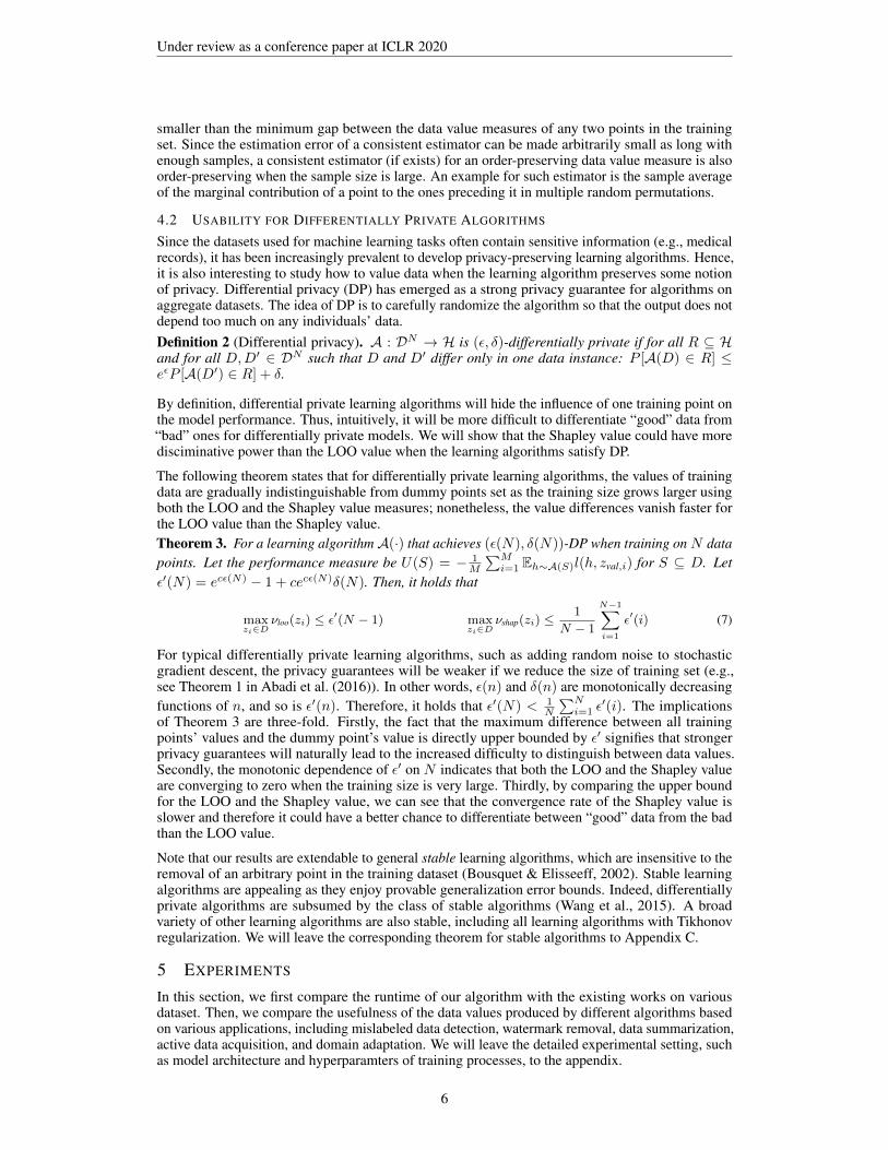
For the pattern-based watermark removal experiment, we consider three settings: two convolutionalnetworks trained on 1000 images from fashion MNIST and 10000 images from MNIST, resepctively,and a ResNet18 model trained on 1000 images from a face recognition dataset, Pubfig-83. Thewatermark ratio is 10% for all three settings. The details about watermark patterns are providedin the appendix. Since for the last two settings, either due to large data size or model size, TMC-Shapley, G-Shapley, and Leave-one-out all fail to produce value estimates in 3 hours, we compare ouralgorithm only with the rest of baselines. The results are shown in Figure 3. We can see that KNN-Shapley achieves similar performance to TMC-Shapley when the time complexity of TMC-Shapleyis acceptable and outperforms all other baselines.

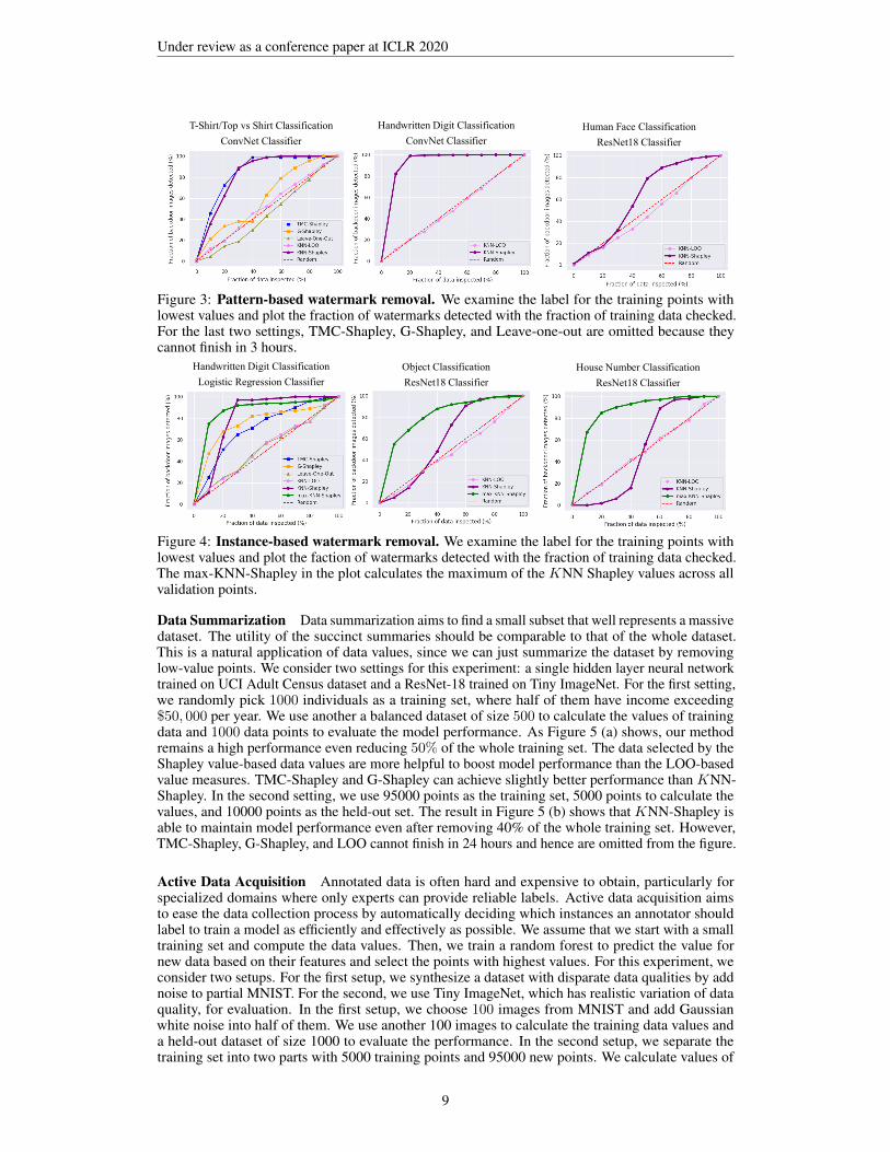
For the instance-based watermark removal experiment, we consider the following settings: a logisticregression model trained on 10000 images from MNIST, a convolution network trained on 3000images from CIFAR-10, and ResNet18 trained on 3000 images from SVHN. The watermark ratiois 10%, 3%, and 3%, respectively. The results of our experiment are shown in Figure 4. Forthis experiment, we found that both watermarks and benign data tend to have low values on somevalidation points; therefore, watermarks and benign data are not quite separable in terms of theaverage value across the validation set. We propose to compute the max value across the validationset for each training point, which we call max-KNN-Shapley, and remove the points with lowestmax-KNN-Shapley values. The intuition is that out-of-distribution samples are inessential to predictall normal validation points and thus the maximum of their Shapley values with respect to differentvalidation points should be low. The results show that the max-KNN-Shapley is more effectivemeasure to detect instance-based watermarks than all other baselines.

8


Human Face Classification

ResNet18 Classifier

Handwritten Digit Classification

ConvNet Classifier

T-Shirt/Top vs Shirt Classification

ConvNet Classifier




1

1

0.97




0.999444

0.999889

0.953




1

1

1

Figure 3: Pattern-based watermark removal. We examine the label for the training points withlowest values and plot the fraction of watermarks detected with the fraction of training data checked.For the last two settings, TMC-Shapley, G-Shapley, and Leave-one-out are omitted because theycannot finish in 3 hours.

House Number Classification

ResNet18 Classifier

Object Classification

ResNet18 Classifier

Handwritten Digit Classification

Logistic Regression Classifier




0.998

0.997778

0.98




1

0.980667

1




1

1

1

Figure 4: Instance-based watermark removal. We examine the label for the training points withlowest values and plot the faction of watermarks detected with the fraction of training data checked.The max-KNN-Shapley in the plot calculates the maximum of the KNN Shapley values across allvalidation points.

Data Summarization Data summarization aims to find a small subset that well represents a massivedataset. The utility of the succinct summaries should be comparable to that of the whole dataset.This is a natural application of data values, since we can just summarize the dataset by removinglow-value points. We consider two settings for this experiment: a single hidden layer neural networktrained on UCI Adult Census dataset and a ResNet-18 trained on Tiny ImageNet. For the first setting,we randomly pick 1000 individuals as a training set, where half of them have income exceeding$50, 000 per year. We use another a balanced dataset of size 500 to calculate the values of trainingdata and 1000 data points to evaluate the model performance. As Figure 5 (a) shows, our methodremains a high performance even reducing 50% of the whole training set. The data selected by theShapley value-based data values are more helpful to boost model performance than the LOO-basedvalue measures. TMC-Shapley and G-Shapley can achieve slightly better performance than KNN-Shapley. In the second setting, we use 95000 points as the training set, 5000 points to calculate thevalues, and 10000 points as the held-out set. The result in Figure 5 (b) shows that KNN-Shapley isable to maintain model performance even after removing 40% of the whole training set. However,TMC-Shapley, G-Shapley, and LOO cannot finish in 24 hours and hence are omitted from the figure.

Active Data Acquisition Annotated data is often hard and expensive to obtain, particularly forspecialized domains where only experts can provide reliable labels. Active data acquisition aimsto ease the data collection process by automatically deciding which instances an annotator shouldlabel to train a model as efficiently and effectively as possible. We assume that we start with a smalltraining set and compute the data values. Then, we train a random forest to predict the value fornew data based on their features and select the points with highest values. For this experiment, weconsider two setups. For the first setup, we synthesize a dataset with disparate data qualities by addnoise to partial MNIST. For the second, we use Tiny ImageNet, which has realistic variation of dataquality, for evaluation. In the first setup, we choose 100 images from MNIST and add Gaussianwhite noise into half of them. We use another 100 images to calculate the training data values anda held-out dataset of size 1000 to evaluate the performance. In the second setup, we separate thetraining set into two parts with 5000 training points and 95000 new points. We calculate values of

9


(a) UCI Census Dataset (b) Tiny ImageNet (c) MNIST with noise (d) Tiny ImageNet

Figure 5: (a-b) Data summarization. We remove low-value points from the ground training set andevaluate the accuracy of the model trained with remaining data. (c-d) Active data acquisition. Wecompute the data values for a small starting set, train a Random forest to predict the values of newdata, and then add the new points with highest values into the starting set. We plot the model accuracychange when combining the starting set with more and more new data added according to differentvalue measures.

2500 data points in the training set based on the other 2500 points. Both Figure 5 (c) and (d) showthat new data selected based on KNN-Shapley value can improve model accuracy faster than the restof baselines.

Domain Adaptation Machine learning models are know to have limited capablity of generalizinglearned knowledge to new datasets or environments. In practice, there is a need to transfer themodel from a source domain where sufficient training data is available to a target domain where fewlabeled data are available. Domain adaptation aims to better leverage the dataset from one domainfor the prediction tasks in another domain. We will show that data values will be useful for this task.Specifically, we can compute the values of data in the source domain with respect to a held-out setfrom the target domain. In this way, the data values will reflect how useful different training pointsare for the task in the target domain. We then train the model based only on positive-value points inthe source domain and evaluate the model performance in the target one. We perform experiments onthree datasets, namely, MNIST, USPS, and SVHN. For the transfer between USPS and MNIST, weuse the same experiment setting as (Ghorbani & Zou, 2019). We firstly train a multinomial logisticregression classifier. We randomly sample 1000 images from the source domain as training set,calculate the values for the training data based on 1000 instances from the target domain, and evaluatethe performance of the model on another 1000 target domain data. The results are summarizedin Table 1, which shows that KNN-Shapley performs better than TMC-Shapley. For the transferbetween SVHN and MNIST, we pick 2000 training data from SVHN, train a ResNet-18 model (Heet al., 2016), and evaluate the performance on the whole test set of MNIST. KNN-Shapley is ableto implement on the data of this scale efficiently while TMC-Shapley algorithm cannot finish in 48hours.Table 1: Domain adapation. We calculate the value of data in source domain based on a validationset from the target domain, and then pick the points with positive values to train the model forperforming prediction tasks in the target domain.

Method MNIST→ USPS USPS→ MNIST SVHN→ MNIST

→ → →KNN-Shapley 31.7%→ 48.40% 23.35%→ 30.25% 9.65%→ 20.25%TMC-Shapley 31.7%→ 44.90% 23.35%→ 29.55% -

KNN-LOO 31.7%→ 39.40% 23.35%→ 24.52% 9.65%→ 11.70%

LOO 31.7%→ 29.40% 23.35%→ 23.53% -

6 CONCLUSION

In this paper, we propose an efficient algorithm to approximate the Shapley value based on KNNproxies, which for the first time, enables the data valuation for large-scale dataset and large modelsize. We demonstrate the utility of the approximate Shapley values produced by our algorithm on avariety of applications, from noisy label detection, watermark removal, data summarization, activedata acquisition, to domain adaption. We also compare with the existing Shapley value approximationalgorithms, and show that our values can achieve comparable performance while the computation ismuch more efficient and scalable. We characterize the advantage of the Shapley value over the LOOvalue from a theoretical perspective and show that it is preferable in terms of predictive power anddiscriminative power under differentially private learning algorithms.

10


REFERENCES

Martin Abadi, Andy Chu, Ian Goodfellow, H Brendan McMahan, Ilya Mironov, Kunal Talwar, andLi Zhang. Deep learning with differential privacy. In Proceedings of the 2016 ACM SIGSACConference on Computer and Communications Security, pp. 308–318. ACM, 2016.

Yossi Adi, Carsten Baum, Moustapha Cisse, Benny Pinkas, and Joseph Keshet. Turning yourweakness into a strength: Watermarking deep neural networks by backdooring. In 27th {USENIX}Security Symposium ({USENIX} Security 18), pp. 1615–1631, 2018.

Olivier Bousquet and Andre Elisseeff. Stability and generalization. Journal of machine learningresearch, 2(Mar):499–526, 2002.

Bryant Chen, Wilka Carvalho, Nathalie Baracaldo, Heiko Ludwig, Benjamin Edwards, TaesungLee, Ian Molloy, and Biplav Srivastava. Detecting backdoor attacks on deep neural networks byactivation clustering. arXiv preprint arXiv:1811.03728, 2018a.

Qingrong Chen, Chong Xiang, Minhui Xue, Bo Li, Nikita Borisov, Dali Kaarfar, and Haojin Zhu.Differentially private data generative models. arXiv preprint arXiv:1812.02274, 2018b.

Amirata Ghorbani and James Zou. Data shapley: Equitable valuation of data for machine learning.arXiv preprint arXiv:1904.02868, 2019.

Ian J Goodfellow, Jonathon Shlens, and Christian Szegedy. Explaining and harnessing adversarialexamples. arXiv preprint arXiv:1412.6572, 2014.

Kaiming He, Xiangyu Zhang, Shaoqing Ren, and Jian Sun. Deep residual learning for imagerecognition. In Proceedings of the IEEE conference on computer vision and pattern recognition,pp. 770–778, 2016.

Ruoxi Jia, David Dao, Boxin Wang, Frances Ann Hubis, Nezihe Merve Gurel, Bo Li, Ce Zhang,Costas Spanos, and Dawn Song. Efficient task-specific data valuation for nearest neighboralgorithms. Proceedings of the VLDB Endowment, 12(11):1610–1623, 2019a.

Ruoxi Jia, David Dao, Boxin Wang, Frances Ann Hubis, Nick Hynes, Nezihe Merve Gurel, Bo Li,Ce Zhang, Dawn Song, and Costas Spanos. Towards efficient data valuation based on the shapleyvalue. arXiv preprint arXiv:1902.10275, 2019b.

Pang Wei Koh and Percy Liang. Understanding black-box predictions via influence functions. InProceedings of the 34th International Conference on Machine Learning-Volume 70, pp. 1885–1894.JMLR. org, 2017.

Yu-Xiang Wang, Jing Lei, and Stephen E Fienberg. Learning with differential privacy: Stability,learnability and the sufficiency and necessity of ERM principle. February 2015.

A PROOF OF THEOREM 2

Theorem 2. For any given D = {z1, . . . , zN}, where zi = (xi, yi), and any given validation pointzval = (xval, yval), assume that z1, . . . , zN are sorted according to their similarity to xval. Let d(·, ·)be the feature distance metric according to which D is sorted. Suppose that P(X,Y )∈D(d(X,xval) ≥d(xi, xval)) > δ for all i = 1, . . . , N and some δ > 0. Then, νshap-knn is order-preserving for all pairsof points in I; νLOO-knn is order-preserving only for (zi, zj) such that max i, j ≤ K.

Proof. The proof relies on dissecting the term E[U(T ∪ {zi}) − U(T ∪ {zj})] and ν(zi) − ν(zj)(ν = νshap-knn, νLOO-knn) in the definition of order-preserving property.

Consider any two points zi, zi+l ∈ D. We start by analyzing E[U(T ∪ {zi}) − U(T ∪ {zi+l})].Let the kth nearest neighbor of xval in T be denoted by T(k) = (x(k), y(k)). Moreover, we will useT(k) ≤d zi to indicate that x(k) is closer to the validation point than xi, i.e., d(x(k), xval) ≤ d(xi, xval).We first analyze the expectation of the above utility difference by considering the following cases:

11


(1) T(K) ≤d zi. In this case, adding zi or zi+l into T will not change the K-nearest neighbors to zval

and therefore U(T ∪ {zi}) = U(T ∪ {zi+l}) = U(T ). Hence, U(T ∪ {zi})− U(T ∪ {zi+l}) = 0.

(2) zi <d T(K) ≤d zi+l. In this case, including the point i into T can expel the Kth nearestneighbor from the original set of K nearest neighbors while including the point i + 1 will notchange the K nearest neighbors. In other words, U(T ∪ {zi})− U(T ) =

1[yi=yval]−1[y(K)=yval]

K and

U(T ∪ {zi+l})− U(T ) = 0. Hence, U(T ∪ {zi})− U(T ∪ {zi+l}) =1[yi=yval]−1[y(K)=yval]

K .

(3) T(K) >d zi+l. In this case, including the point i or i + 1 will both change the original Knearest neighbors in T by excluding the Kth nearest neighbor. Thus, U(T ∪ {zi}) − U(T ) =1[yi=yval]−1[y(K)=yval]

K and U(T ∪ {zi+l})− U(T ) =1[yi+l=yval]−1[y(K)=yval]

K . It follows that U(T ∪{zi})− U(T ∪ {zi+l}) = 1[yi=yval]−1[yi+l=yval]

K .

Combining the three cases discussed above, we have

E[U(T ∪ {zi})− U(T ∪ {zi+l})] (8)

= P (T(K) ≤d zi)× 0 + P (zi <d T(K) ≤d zi+l)1[yi = yval]− 1[y(K) = yval]

K

+ P (T(K) >d zi+l)1[yi = yval]− 1[yi+l = yval]

K(9)

= P (zi <d T(K) ≤d zi+l)1[yi = yval]− 1[y(K) = yval]

K

+ P (T(K) >d zi+l)1[yi = yval]− 1[yi+l = yval]

K(10)

Note that removing the first term in (10) cannot change the sign of the sum in (10). Hence, whenanalyzing the sign of (10), we only need to focus on the second term:

P (T(K) >d zi+1)1[yi = yval]− 1[yi+l = yval]

K(11)

Since P (T(K) >d zi+1) =∑Nk=N−K+1 P (Z >d zi+1)

k, the sign of (11) will be determined by thesign of 1[yi = yval]− 1[yi+l = yval]. Hence, we get(

E[U(T ∪ {zi})− U(T ∪ {zi+1})])×(1[yi = yval]− 1[yi+l = yval]

)> 0 (12)

Now, we switch to the analysis of the value difference. By Theorem 1, it holds for the KNN Shapleyvalue that

νshap-knn(zi)− νshap-knn(zi+l) (13)

=

i+l−1∑j=i

min{K, j}jK

(1[yj = yval]− 1[yj+1 = yval]

)(14)

=min{K, i}

iK1[yi = yval] +

i+l−2∑j=i

(min{K, j + 1}

(j + 1)K− min{K, j}

jK

)1[yj+1 = yval]

− min{K, i+ l − 1}(i+ l − 1)K

1[yi+l = yval] (15)

Note that min{K,j+1}(j+1)K − min{K,j}

jK < 0 for all j = i, . . . , i + l − 2. Thus, if 1[yi = yval] = 1

and 1[yi+l = yval] = 0, the minimum of (15) is achieved when 1[yj+1 = yval] = 1 for allj = i, . . . , i + l − 2 and the minimum value is min{K,i+l−1}

(i+l−1)K , which is greater than zero. On theother hand, if 1[yi = yval] = 0 and 1[yi+l = yval] = 1, then the maximum of (15) is achieved when1[yj+1 = yval] = 0 for all j = i, . . . , i+ l − 2 and the maximum value is −min{K,i+l−1}

(i+l−1)K , which isless than zero.

Summarizing the above analysis, we get that νshap-knn(zi) − νshap-knn(zi+l) has the same sign as1[yi = yval] − 1[yi+l = yval]. By (12), it follows that νshap-knn(zi) − νshap-knn(zi+l) also shares thesame sign as E[U(T ∪ {zi})− U(T ∪ {zi+1})].

12


To analyze the sign of the KNN LOO value difference, we first write out the expression for the KNNLOO value difference:

νloo-knn(zi)− νloo-knn(zi+l) =

1K (1[yi = yval]− 1[yi+l = yval]) if i+ l ≤ K1K (1[yi = yval]− 1[yK+1 = yval]) if i ≤ K < i+ l

0 if i > K(16)

Therefore, νloo-knn(zi) − νloo-knn(zi+l) has the same sign as 1[yi = yval] − 1[yi+l = yval] andE[U(T ∪ {zi})− U(T ∪ {zi+1})] only when i+ l ≤ K.

B PROOF OF THEOREM 3

We will need the following lemmas on group differential privacy for the proof of Theorem 3.

Lemma 2. If A is (ε, δ)-differentially private with respect to one change in the database, then A is(cε, cecεδ)-differentially private with respect to c changes in the database.

Lemma 3 (Jia et al. (2019b)). For any zi, zj ∈ D, the difference in Shapley values between zi andzj is

νshap(zi)− νshap(zj) =1

N − 1

∑T⊆D\{zi,zj}

U(T ∪ {zi})− U(T ∪ {zj})(N−2|T |) (17)

Theorem 3. For a learning algorithmA(·) that achieves (ε(N), δ(N))-DP when training on N datapoints. Let the performance measure be U(S) = − 1

M

∑Mi=1 Eh∼A(S)l(h, zval,i) for S ⊆ D. Let

ε′(N) = ecε(N) − 1 + cecε(N)δ(N). Then, it holds that

maxzi∈D

νloo(zi) ≤ ε′(N − 1) maxzi∈D

νshap(zi) ≤1

N − 1

N−1∑i=1

ε′(i) (7)

Proof. Let S′ be the set with one element in S replaced by a different value. Let the probabilitydensity/mass defined by A(S′) and A(S) be p(h) and p′(h), respectively. Using Lemma 2, for anyzval we have

Eh∼A(S)l(h, zval) =

∫ 1

0

Ph∼A(S)[l(h, zval) > t]dt (18)

≤∫ 1

0

(ecεPh∼A(S′)[l(h, zval) > t] + cecεδ)dt (19)

= ecεEh∼A(S′)[l(h, zval)] + cecεδ (20)

It follows that

Eh∼A(S)l(h, zval)− Eh∼A(S′)[l(h, zval)] ≤ (ecε − 1)Eh∼A(S′)[l(h, zval)] + cecεδ (21)

≤ ecε − 1 + cecεδ (22)

By symmetry, it also holds that

Eh∼A(S′)l(h, zval)− Eh∼A(S)[l(h, zval)] ≤ (ecε − 1)Eh∼A(S)[l(h, zval)] + cecεδ (23)

≤ ecε − 1 + cecεδ (24)

Thus, we have the following bound:

|Eh∼A(S)l(h, zval)− Eh∼A(S′)[l(h, zval)]| ≤ ecε − 1 + cecεδ (25)

13


Denoting ε′ = ecε − 1 + cecεδ. For the performance measure that evaluate the loss averaged acrossmultiple validation points U(S) = − 1

M

∑Mi=1 Eh∼A(S)l(h, zval,i), we have

|U(S)− U(S′)| ≤ ε′ (26)

Making the dependence on the training set size explicit, we can re-write the above equation as

maxzi,zj∈D,T⊆D\{zi,zj}

|U(T ∪ zi)− U(T ∪ zj)| ≤ ε′(|T |+ 1) (27)

By Lemma 3, we have for all zi, zj ∈ D,

νshap(zi)− νshap(zj) ≤1

N − 1

N−2∑k=0

∑T⊆D\{zi,zj},|T |=k

ε′(k + 1)(N−2k

) (28)

=1

N − 1

N−2∑k=0

ε′(k + 1) (29)

=1

N − 1

N−1∑k=1

ε′(k) (30)

As for the LOO value, we have

νloo(zi)− νloo(zj) = U(D \ {zj})− U(D \ {zi}) (31)

≤ ε′(N − 1) (32)

C COMPARING THE LOO AND THE SHAPLEY VALUE FOR STABLE LEARNINGALGORITHMS

An algorithm G has uniform stability γ with respect to the loss function l if ‖l(G(S), ·) −l(G(S\i), ·)‖∞ ≤ γ for all i ∈ {1, · · · , |S|}, where S denotes the training set and S\i denotesthe one by removing ith element of S.

Theorem 4. For a learning algorithm A(·) with uniform stability β = Cstab|S| , where |S| is the

size of the training set and Cstab is some constant. Let the performance measure be U(S) =

− 1M

∑Mi=1 l(A(S), zval,i). Then,

maxzi∈D

νloo(zi)− νloo(z∗) ≤ Cstab

N − 1(33)

and

maxzi∈D

νshap(zi)− νshap(z∗) ≤ Cstab(1 + log(N − 1))

N − 1(34)

Proof. By the definition of uniform stability, it holds that

maxz,zj∈D,T⊆D\{zi,zj}

|U(T ∪ {zi})− U(T ∪ {zj})| ≤Cstab

|T |+ 1(35)

Using Lemma 3, we have we have for all zi, zj ∈ D,

νshap(zi)− νshap(zj) (36)

≤ 1

N − 1

N−2∑k=0

∑T⊆D\{zi,zj},|T |=k

Cstab(N−2k

)(k + 1)

(37)

=1

N − 1

N−2∑k=0

Cstab

k + 1(38)

14


Recall the bound on the harmonic sequences

N∑k=1

1

k≤ 1 + log(N)

which gives us

νshap(zi)− νshap(zj) ≤Cstab(1 + log(N − 1))

N − 1

As for the LOO value, we have

νloo(zi)− νloo(zj) = U(D \ {zj})− U(D \ {zi}) ≤Cstab

N − 1(39)

D ADDITIONAL EXPERIMENTS

D.1 REMOVING DATA POINTS OF HIGH VALUE

We remove training points from most valuable to least valuable and evaluate the accuracy of themodel trained with remaining data. The experimental setting, including datasets and models, is thesame as that for the data summarization experiment. Figure 6 compares the power of different datavalue measures to detect high-utility data. We can see that removing high-value points based onKNN-Shapley, G-Shapley, and TMC-Shapley can all significantly reduce the model performance.It indicates that these three heuristics are effective in detecting most valuable training points. OnUCI Census, TMC-Shapley achieves the best performance and KNN-Shapley performs similarly toG-Shapley. On Tiny ImageNet, both TMC-Shapley and G-Shapley cannot finish in 24 hours and aretherefore omitted from comparison. Compared with the random baseline, KNN-Shapley can lead toa much faster performance drop when removing high-value points.

(a) UCI Census Dataset (b) Tiny ImageNet

Figure 6: (a-b) We remove high-value points from the ground training set and evaluate the accuracyof the model trained with remaining data.

D.2 RANK CORRELATION WITH GROUND TRUTH SHAPLEY VALUE

We perform experiments to compare the ground truth Shapley value of raw data and the valueestimates produced by different heuristics. The ground truth Shapley value is computed usingthe group testing algorithm in (Jia et al., 2019b), which can approximate the Shapley value withprovable error bounds. We use a fully-connected neural network with three hidden layers as thetarget model. Following the setting in (Jia et al., 2019b), we construct a size-1000 training set usingMNIST, which contains both benign and adversarial examples, as well as a size-100 validation set

15


with pure adversarial examples. The adversarial examples are generated by the Fast Gradient SignMethod (Goodfellow et al., 2014). This construction is meant to simulate data with different levels ofusefulness. In the above setting, the adversarial examples in the training set should be more valuablethan the benign data because they can improve the prediction on adversarial examples. Note that theKNN-Shapley computes the Shapley value of deep features extracted from the penultimate layer.

The rank correlation of KNN-Shapley and G-Shapley with the ground truth Shapley value is 0.08and 0.024 with p-value 0.0046 and 0.4466, respectively. It shows that both heuristics may not beable to preserve the exact rank of the ground truth Shapley value. Since TMC-Shapley cannot finishin a week for this model and data size, we omit it from comparison. We further apply some localsmoothing to the values and check whether these heuristics can produce large values for data groupswith large Shapley values. Specifically, we compute 1 to 100 percentiles of the Shapley values, findthe group of data points within each percentile interval, and compute the average Shapley value aswell as the average heuristic values for each group. The rank correlation of the average KNN-Shapleyand the average G-Shapley with the average ground truth Shapley value for these data groups are0.22 and -0.002 with p-value 0.0293, 0.9843, respectively. We can see that although ignoring the datacontribution for feature learning, KNN-Shapley can better preserve the rank of the Shapley value ina macroscopic level than G-Shapley.

E EXPERIMENT DETAILS

E.1 PATTERN-BASED WATERMARK REMOVAL

We adopted two types of patterns: one is to change the pixel values at the corner of an image Chen et al.(2018a), another is to blend a specific word (like ”TEST”) in an image, as shown in Figure 7a. Thefirst pattern is used in the experiments on fashion MNIST and MNIST, which contain single channelimages. The second pattern is used in the experiment on Pubfig-83, which contains multi-channelimages.

(a) (b)

Figure 7: (a) Examples of pattern-based watermarks. Specifically, after an image is blended with the“TEST” pattern, it is classified as the target label, e.g, an “automobile” on CIFAR-10. (b) Example ofinstance-based watermarks, which are typically chosen as some out-of-distribution data with specificassigned labels.

Table 2 shows the prediction accuracy of the watermarked model on both benign and watermarkinstances. The results indicate that the amount of watermarks we added can help successfully claimthe ownership of the data source.

Model Accuracy Handwritten Digit Object House Number(Logistic Regression) (ResNet18) (ResNet18)

Watermarked Model on Benign Data 0.997778 0.980667 1

Watermarked Model on Watermark Data 0.98 1 1

Table 2: Model accuracy for pattern-based watermark removal experiment.

E.2 INSTANCE-BASED WATERMARK REMOVAL

We used the same watermarks as Adi et al. (2018), which contains a set of abstract images withspecific assigned labels. The example of a trigger image is shown in Figure 7b.

16


E.3 DATA SUMMARIZATION

For the experiment on UCI Adult Census dataset, we train the same multilayer perceptron modeas Chen et al. (2018b). The network architecture is displayed in Table 3.

Model for Adult Census DatasetFC(6) + Sigmoid

FC(100) + Sigmoid

Table 3: Model for evaluating the data meaning in Data Summarization

For the experiment on Tiny ImageNet, we fine-tune the pretrained ResNet18 from He et al. (2016).We train the ResNet18 with 15 epochs and learning rate 0.001 and the model achieves an accuracy of77.95% on the training set. Then, we extract the deep features of the training set and calculate theirShapley values. When evaluating the model performance on the summarized dataset, we re-train theResNet18 with 30 epochs and learning rate 0.01.

E.4 DOMAIN ADAPTATION

As to the domain adaptation between MNIST and USPS, we train a multinomial logistic regressionclassifier. For transfer from SVHN to MNIST, we train a ResNet18 model using 15 epochs andlearning rate 0.001 on SVHN, since multinomial logistic regression is too simple to perform well inthis setting.

17

an empirical and comparative analysis of data valuation …

Documents