An Empirical Analysis of Resampled Efficiency

A Thesis

Submitted to the Faculty

of the

WORCESTER POLYTECHNIC INSTITUTE

in partial fulfillment of the requirements for the

Professional Masters Degree in Financial Mathematics

By

Jasraj Kohli

_________________________

Date: May 1, 2005

APROVED:

____________________________

Professor Arthur C. Heinricher, Jr., Thesis Advisor

____________________________

Professor Bogdan Vernescu, Head, Mathematical Sciences Department

Abstract

Michaud introduced resampled efficiency as an alternative and improvement to

Markowitz mean-variance efficiency. While resampled efficiency is far from becoming

the standard paradigm of capital allocation amongst risky assets, it has nonetheless

gained considerable ground in financial circles and become a fairly debated portfolio

construction technique.

This thesis applies Michaud’s techniques to a wide array of stocks and tries to validate

claims of performance superiority of resampled portfolios. While there seems to be no

conclusive advantage or disadvantage of using resampling as a technique to obtain better

returns, resampled portfolios do seem to offer higher stability and lower transaction costs.

i

Acknowledgements

I would like to thank the faculty and students of the WPI Mathematics Department for

their help and support, Dr. Arthur C. Heinricher for guiding me through the various

stages of my project and Dr. Domokos Vermes for guiding me through my degree.

I would especially like to thank the graduate committee whose support made this degree

financially possible.

ii

Table of Contents Abstract….………………………………………………………………………………...i Acknowledgments………………………………………………………………………..ii

1 Mean Variance Efficiency...........................................................................................1

1.1 Introduction to Markowitz Mean Variance Efficiency………………………..1 1.2 Criticisms of Mean-Variance Efficiency……………………………………...3

2 The Resampled Efficient Frontier…………………………………………………..7

2.1 Introduction……………………………………………………………………7 2.2 Procedure to generate Resampled Efficient Frontier………………………….7 2.3 Statistically equivalent portfolios……………………………………………..9 2.4 Advantages, Disadvantages………………………………………………….10

3 Empirical Study:……………………………………………………………………12

3.1 Procedure to obtain Mean Return MVE Portfolio…………………………...12 3.2 Rationale behind approach adopted………………………………………….13 3.3 In sample testing, Obtaining Results………………………………………...14

4 Results and Analysis:…………………………………………………………….....16

4.1 Results………………………………………………………………………..16 4.2 Analysis of resampled efficiency performance………………………………17 4.3 Trends Observed……………………………………………………………..18

5 Investment Recommendations:……………………………………………………19

6 Conclusion:……………………………………………………………………….....20 7 References:…………………………………………………………………………..21 Appendix A: Stock Data:………………………………………………………………22

Appendix B: Matlab Code:…………………………………………………………….23

Appendix C: Detailed Results:…………………………………………………………28

iii

1 Mean Variance Efficiency

1.1 Introduction to Markowitz Mean Variance Efficiency

Mean Variance Efficiency refers to the classical approach to solve the portfolio allocation

problem as proposed by Harry Markowitz [2]. Given a portfolio with N assets with a

fraction of total wealth xi invested in each asset with return Ri (a random variable), the

expected return on the portfolio is the weighted average of the individual expected

returns:

[ ] [ ] ∑∑==

====N

iii

N

iiipp xRExREE

11µ µTx .

Correspondingly, the portfolio risk is the variance (or standard deviation) of the return on

the portfolio: [2]

[ ] === ∑∑==

N

ijiji

N

jpp xxRVarV

11

σ CxxT

Where C is the n x n covariance matrix with entries

[ ]))(( jjiiij RRE µµσ −−=

Accordingly, given the expected returns, standard deviations of returns and correlations

of returns on assets, Markowitz Mean Variance efficiency seeks to find portfolio weights

which minimizes risk for a given level of return and maximizes return for a given level of

risk. Such portfolios are called efficient and the set of all efficient (feasible) portfolios is

called the efficient frontier. It reduces to a mathematical optimization problem which may

be stated as:

1

a) Minimize , subject to specified level of return and , or pV =pE 11

=∑=

N

iix

b) Maximize , subject to specified level of risk and , or pE =pV 11

=∑=

N

iix

Additionally, we may impose constraints such as:

• (No asset may be shorted) ixi ∀≥ ,0

• (No asset may have more than a certain fraction of total investment) ifxi ∀≤ ,

Any such constraint shrinks the feasible set and pulls the efficient frontier inwards in the

risk return space.

Alternatively, the optimization problem may be stated as:

Minimize pEp EVU λ−= , subject to 11

=∑=

N

iix

Here, U is the utility function and the parameter Eλ is a measure of the risk aversion for

the investor (reciprocal of the risk tolerance). This definition helps in customizing the

portfolio allocation problem to the risk aversion of the individual investor. At the same

time, however, no clear standards exist on the quantification of Eλ .

Standard algorithms (linear programming/quadratic programming) are available to

compute the efficient frontier with or without short-selling/borrowing constraints.

Markowitz extended the technique of quadratic programming to develop the “critical line

algorithm” [7] to solve the optimization problem. The main drawback to this algorithm is

that it does not solve for specific points on the efficient frontier, but rather provides a

sample of the portfolios on the efficient frontier. It does not provide a portfolio for a

specified return; therefore, very few commercial packages use this algorithm. Matlab’s

2

frontcon uses quadratic programming to solve the same problem by solving for optimal

portfolios with specified returns along the efficient frontier and has been used for this

project.

1.2 Criticisms of Mean-Variance Efficiency

There are a number of objections to MV Efficiency [1]

(1) Non Variance Risk Measures: Variance is not uniformly accepted as an appropriate

measure of the risk of a portfolio. This criticism by itself raises serious doubts about

the central role given to mean-variance efficient portfolios in both investment theory

and practice. Various other risk definitions exist. Downside risk measures of

variability such as mean-semivariance or mean - semi standard deviation of return,

the mean absolute deviation and range measures could be good alternatives to the

traditional risk measure variance or standard deviation [5].

Mean - semivariance is defined as the variance of returns on a portfolio below the

mean return level. This may be generalized to target semivariance where returns

below a target, such as zero or the risk free rate (and not just the mean) contribute

towards calculation of risk.

Mean absolute deviation for a sample of N returns, R1…RN, is defined as

∑=

−=N

iiR

NMD

1

1 µ

Where, ∑=

=N

iiR

N 1

1µ .

Just as in the case of target semivariance, µ may be replaced by a specific return

level.

3

One of the most commonly used alternative risk measure is Value at Risk (VaR). It

records the actual loss that would occur if the returns were in the worst x % of the

distribution (where x is the threshold). More precisely VaR is an amount (say D

dollars), where the probability of losing more than D dollars is p over some future

time interval, T days.

(2) Utility Function Optimization: Markowitz MV efficiency is consistent with

maximization of expected utility of terminal wealth, which acts as a rationale for

financial investors to choose MV efficient portfolios. However, this is justified only

in one of the following two conditions. In the first case utility of terminal wealth is

maximized when returns are normally distributed. While the returns may be

distributed symmetrically for diversified equity portfolio and index returns, the

distribution is not precisely normal. Further, asset classes such as fixed income

indexes are asymmetric. MV Efficiency also maximizes terminal wealth utility for

quadratic utility functions. There is, however, a major limitation to the use of

quadratic utility functions to mirror investment tendencies. This is because quadratic

utility declines as a function of positive wealth increments beyond a certain point and

therefore quadratic utility functions find better applicability in approximating

maximum wealth in a given restricted range. Accordingly then, MV efficiency does

not always achieve utility function maximization.

(3) Multiperiod Investment Horizons: Markowitz’ mean-variance efficient paradigm is a

one-period model. Most institutional and individual investors typically have a ten-

4

year, twenty-year, or even longer investment horizon. Markowitz himself has shown

that mean-variance efficient portfolios need not be efficient in the long run [7].

Additionally, mean-variance efficient portfolios in the upper part of the efficient

frontier are less efficient in the long run. To address these problems, some have

suggested reformulating the mean-variance analysis using longer time-periods

consistent with the investor's investment horizon. However, if one were to consider a

ten-year or twenty- year return as one observation, we would have very few

observations from the U.S. (or any other) capital markets for estimation (of the

efficient frontier) purposes. Additionally, increasing historic data will reduce the

accuracy of forecasting for a short term period.

(4) Instability and Ambiguity: In practice, mean-variance efficient portfolios have been

found to be quite unstable: small changes in the estimated parameter inputs lead to

large changes in the implied portfolio holdings (“Instability and Ambiguity”). The

practical implementation of the mean-variance efficient paradigm requires

determination of the efficient frontier. This requires three inputs: expected returns of

the assets, expected correlation among these assets, and expected variance of these

assets (individually). Typically, these input parameters are estimated using historical

data. Researchers, as Jobson and Korkie [6], have found that estimation errors in

these input parameters can overwhelm the theoretical benefits of the mean-variance

paradigm. These estimation errors may result from uncharacteristically low or high

recent returns for a certain set of securities which then results in much higher (or

5

lower) allocation. In effect, small changes in the inputs often lead to very different

portfolio weights and accordingly wildly diverging efficient frontiers.

6

2 The Resampled Efficient Frontier

2.1 Introduction

While the above criticisms of MV efficiency are noteworthy, practitioners pay limited

attention to them. To start off, efficient frontiers of non variance risk measures do not

look significantly different from the Markowitz efficient frontiers except in cases of asset

classes such as options, where returns are not approximately symmetric and MV

efficiency is a bad allocation choice in the first place. Next, utility functions have

practical limitations when it comes to using them as a basis for optimization definition.

This is a consequence of lack of feasible and viable algorithms for computation of

optimal portfolios that would conform to the utility function, since the utility function

may very well require non linear optimization solutions. For these reasons, MV

efficiency continues to remain a favorite allocation strategy. However, in 1998, Richard

Michaud proposed “Resampling” to tackle at least one of the primary criticisms, i.e.

“Instability and Ambiguity” [1]. This gave rise to the resampled efficient frontier.

2.2 Procedure to generate Resampled Efficient Frontier

The resampled efficient frontier is generated using the following procedure

• Estimate the expected returns (µ) and the variance – covariance matrix (C).

Suppose there are m assets.

• Assuming no short selling is allowed, solve for the minimum-variance portfolio.

Call the expected return of this portfolio L. Solve for the maximum return

portfolio. Call the expected return of this portfolio H.

7

• Choose the number of discrete increments, in returns, for characterizing the

frontier.

• For L=a and H=b, choose K increments and δ = (a-b)/K. This means that we

evaluate the frontier at expected return = {a, a + δ, ... , b - δ, b}, that is K different

points.

• We will represent the ‘frontier’ as FK, where ‘FK’ consists of K row vectors

containing weights of the K portfolios along the efficient frontier. So for m assets,

FK is K x m (rows represent the number of points on the frontier and columns are

the asset weights).

• Now begin the Monte Carlo analysis. Assume a multivariate normal distribution

with mean vector µ and variance – covariance matrix C, and draw m returns as

many times as necessary so as to create a big sample which may be used as an

approximation for the return distribution. With the generated data, calculate the

simulated means (µ*) and variance-covariance matrix (C*).

• Now, C* and C are “statistically equivalent” [6]. Using C*, calculate the

minimum variance portfolio (expected return L*) and the maximum expected

return portfolio (expected return H*). Use these to determine the size of the

expected return increments.

• Calculate the efficient portfolio weights at each of these K points

• With this information, we now have FK,i. This is the same dimension, K x m.

• Repeat the simulations S times, so that we have S FK,is.

• Remove any portfolios that have an unusually high (or low) risk level in

comparison to other statistically equivalent portfolios to get the modified FK,is

8

• Average the modified FK,is to get the Resampled weights. We can now draw the

resampled efficient frontier, by using the original means and variances combined

with the new weights. (Refer to Figure 1.)

2.3 Statistically equivalent portfolios

The process of resampling generates K portfolios each time. Each of these portfolios

corresponds to a return level on the original MV efficient frontier. Any two portfolios

which correspond to the same return level on the original MV efficient frontier are

termed statistically equivalent [6]. Alternatively, statistically equivalent portfolios may

be defined as those that have the same risk – return trade-off [3]. This would mean that

any two statistically equivalent portfolios minimize the utility function, pEp EVU λ−= ,

for the same level of risk aversion, Eλ . It is important to note that two statistically

equivalent portfolios, as defined by Michaud, are neither necessarily the same in terms of

expected return nor in terms of risk. Typically, statistically equivalent resampled

portfolios corresponding to MV efficient portfolios with returns in close proximity of

least return MV efficient portfolio have similar risk and return levels. However, as one

ventures towards higher returns, such similarities decrease.

9

H

2.4 Advantages, Disadvantages

Advantages [1]:

The advantage of resampled efficiency is its use of available data to produce more

intuitive portfolio allocations which are less sensitive to input perturbations. This is

because the resampled efficient portfolio is more diversified and intuitively less risky

than one on a corresponding Markowitz efficient frontier. Resampled efficiency therefore

uses investment information in a more robust manner than MV efficiency. Also, because

resampled efficiency is an averaging process, it is very stable. Small changes in the inputs

are generally associated with only small changes in the optimized portfolios. The

resampling process therefore provides protection against over fitting of data.

L

MV Efficient Frontier

Return “Statistically Equivalent” Portfolios

Resampled Efficient Frontier

Risk

Figure 1: Resampled and MVE Frontiers

10

Disadvantages:

The biggest disadvantage of resampling comes from the fact that it does not have a sound

theoretical foundation. Though the process creates “statistically equivalent” portfolios, it

cannot be argued theoretically that the resampled portfolio outperforms the MV efficient

portfolio. In fact, there is no statistical reasoning as to why the resampled portfolios are

averaged (which is the only addition to the process of resampling as introduced by Jobson

and Korkie [6]). Further, Michaud offers little reasoning for why the comparison of MV

efficient portfolio and its statistically equivalent resampled portfolio is valid in the first

place given that they are neither identical in risk nor return. Additionally, the so called

definition of statistically equivalent portfolios is not a uniformly accepted one. Also, the

process of resampling uses the original estimate of mean return vector, µ, and variance -

covariance matrix C, to simulate µ * and C* and evaluate the resampled efficient

frontier, thereby amplifying any errors in the original estimation (even if they are minor

to begin with).

11

3 Empirical Study:

3.1 Procedure

This superiority of resampled efficiency is assessed by studying

(a) Return advantage

(b) Transaction cost advantage, for transaction costs resulting from periodic

rebalancing

In calculating resampled efficient frontiers, it is assumed that no short selling is allowed

and additionally any resampled portfolios which have unusually high or low risk

associated with them (in comparison to other statistically equivalent resampled

portfolios) are removed. The process of resampling then, leads to a large number of

resampled efficient portfolios that are statistically equivalent to corresponding MV

efficient portfolios. One should therefore be able to verify claims of performance

superiority of resampled efficiency, on average, for any given resampled portfolio. An

inexhaustible number of such portfolios are available for testing corresponding to each

efficient frontier for any array of stocks. Performance for a resampled portfolio

corresponding to the MV efficient portfolio with return equaling the average of the

highest and lowest possible MV efficient returns is tested. This portfolio on the

Markowitz efficient frontier may be defined as Mean Return MVE portfolio. The

corresponding resampled statistical equivalent will be referred to as Mean Resampled

portfolio (this is somewhat of a misnomer, but helps in reducing verbosity).

12

To test the return advantage, the above process is repeated for sixty portfolios of seventy

five stocks each. In all, the theory is put to test for 4500 stocks using 600 days of data

(January 2nd, 2001 to May 27th, 2003).

To test the transaction cost advantage, transaction costs are evaluated for rebalancing the

Mean Return MVE and Mean Resampled portfolio. In all four portfolios of 20 stocks are

chosen at random from the many stocks available.

3.2 Rationale behind the approach

There are a number of reasons for concentrating on the mean return MVE portfolio. At

the very least, since resampled efficiency does not claim to perform in a restricted area of

the efficient frontier, so hypothesis testing should work for any resampled portfolio. The

resampled portfolios statistically equivalent to those in the lower part of the efficient

frontier are however very similar to the MVE portfolios in terms of both return and risk

level. The process of resampling would therefore offer little return advantage for these

lower return levels and be of little interest. On the other extreme MVE portfolios with

high risk and high return would need a very high level of risk tolerance and accordingly

not conform to most utility functions. Again, this would lead to a study of portfolios of

little practical investment value and wildly diverging behavior. This leaves us with

resampled portfolios in close proximity to the statistical equivalent of mean return MVE

portfolio that offer the best compromise in terms of risk and return.

13

Ideally, one may wish to specify an exact level of return or certain risk. However, that

may not necessarily correspond to one of the portfolio points on the MVE frontier. This

would need some adjustment and further approximation of results. Even if one was to

obtain a MVE portfolio corresponding to a given return for one frontier, the same may

not be possible for another. In fact, the specified return or risk may very well be beyond

the feasible MVE portfolios for a given frontier. Indeed any portfolio which is close to

the MVE portfolio may be used for the study. However, this is unlikely to yield

dramatically different results.

3.3 In-sample testing

After going through rigorous data splitting, cleaning and recombining clean data (Refer

to Appendix B: Matlab Code), an efficient frontier is calculated for a portfolio of 75

stocks chosen at random from the available stocks. This is done using the first 300 days

of stock data (January 2nd, 2001 to March 18th, 2002), following which the resampled

efficient frontier is constructed using the procedure mentioned in 3.1. The Mean Return

MVE portfolio and mean resampled portfolio are then used for In-sample testing. The

evolution of the portfolios is tracked over the next 300 days (March 19th, 2002 to May

27th, 2003, without rebalancing) in order to evaluate compare portfolio performance.

This process is repeated until all available stocks are exhausted, thereby constructing

sixty such portfolios. In order to evaluate relative performance, multiple approaches are

available. A naïve approach would simply give advantage to the higher value portfolio at

the end of the second 300 day period. This study, however, makes use of Exponential

14

Weighted Moving Average of the value difference between the Mean MVE portfolio and

its statistically equivalent resampled portfolio. A positive EWMA of the value difference

between a mean resampled and mean MVE portfolio would indicate superiority of

resampled efficiency.

In the second study, transaction costs are evaluated for rebalancing the Mean Return

MVE and Mean Resampled portfolio. In all four portfolios of 20 stocks are chosen at

random from the stocks available. Then the Mean Return MVE portfolio and Mean

Resampled portfolio are evaluated for those portfolios on December 12th, 2002 and at

subsequently at 30 day intervals (January 16th 2003, March 3rd 2003, April 14th 2003 and

May 27th 2003). Transaction costs resulting from rebalancing the portfolios on those

dates are calculated to assess which portfolio offers lower net transaction costs.

15

4 Results and Analysis:

4.1 Results

For EWMA of the value difference between the mean resampled and mean return MVE

portfolio, the mean resampled portfolio outperforms in 23 of the 60 portfolios (Refer to

Appendix C for detailed results).

In the worst case scenario, the mean resampled portfolio on average makes 42 cents less

than the mean return MVE portfolio for every dollar invested (on a daily basis) and in the

best case scenario, it makes 46 cents more. The mean of EWMAs is -0.0215367 (which

implies that the mean resampled portfolio makes 2.15 cents less on a daily basis) and the

median EWMA is -0.0170125 (which implies that the mean resampled portfolio makes

1.7 cents less on a daily basis). Figure 2 shows the distribution of EWMAs.

Figure 2: EWMA distribution

16

When the rebalancing costs are assessed (adding up transaction costs for each of the four

rebalancing dates), the mean resampled portfolio offers lower net transaction costs for

three of the four randomly chosen portfolios. In the one case that mean MVE portfolio

does actually offer lower net transaction costs, the difference is of the order of one

thousandth of the advantage offered by the mean resampled portfolio in the other three

cases. This may very well be attributed to rounding errors and additionally the MVE

portfolio being unusually diversified and stable to begin with (Details in Appendix C).

4.2 Analysis of resampled efficiency performance

Contrary to Michaud’s claim, resampled efficiency seems to offer little advantage and

ironically, on average, at a disadvantage when compared to the mean variance efficiency

in terms of offering higher returns. Michaud’s published claims rest on subjective

arguments and exposition by using a very small data set. There is no theoretically sound

explanation as to why resampling must work. It does not come across as a big surprise

then, that resampled efficiency does not outperform Markowitz efficiency. To begin with,

resampled efficiency does not offer a solution for MVE limitation of not being able to

account for multi period investment horizons. In fact, it would be fair to say that there is

no fool proof or even nearly fool proof mechanism to guarantee returns above the risk

free rate for a long term period. In this respect resampling also fails.

17

In fact, the resampled efficient frontier is no different from an inefficient mean variance

frontier, in terms of risk and return levels. Superiority of resampled efficiency would then

imply that the portfolio compositions, even though they offer similar return and risk, are

better equipped to deal with market fluctuations. However, there are far too many factors

which are impossible to ignore in favor of such a theory. Constant current events and

company releases often necessitate that any portfolio, no matter how well thought or

resampled, must be reallocated to conform to expected returns based on key assumptions

of the future, and not past historical returns. Further, the averaging process may lead to

the averaging of very high risk portfolios. Though this study removes such outliers (those

with very high risk levels are removed) little benefit seems to have been derived in terms

of obtained results as far as obtaining better returns is concerned.

However, when it comes to assessing transaction costs, the mean resampled portfolio

offers a marked advantage over the MVE portfolio. Thus resampling is indeed an

averaging process leading to increased diversification and somewhat incorporating mean

variance efficiency, which gives it stability and accordingly better returns, this is simply

not observed.

4.3 Observable trends

There are no observable trends in terms of returns obtained on the mean MVE and mean

resampled portfolio. However, when 30 day periodic rebalancing is done, the mean

resampled portfolio usually offers lower transaction costs.

18

5 Investment Recommendations

The most tangible benefit of resampling is that it helps in giving lower net transaction

costs. This may be of significant advantage to any investor seeking to maintain a well

balanced portfolio by incorporating any newly available information over pre specified

intervals.

Even then, resampling must be combined with day to day market knowledge so as to

bring the portfolio in sync with changing market conditions. A sudden and unexpected

market fluctuation may, for example, necessitate immediate rebalancing. Additionally

investors may need to tweak the amounts invested in individual securities based on their

own intuition.

19

6 Conclusion

Resampling is an effective mechanism for portfolio construction which seems to provide,

on average, lower transaction costs when rebalancing is done. It does not, however,

decidedly point towards any higher (or lower) returns in comparison to the Markowitz

portfolios.

Thus, any investor who seeks to reduce transaction costs in the process of rebalancing (as

is the case with many actively trading firms) may look towards resampling as a way to do

so, simultaneously taking into account other factors as company releases, press reports

and other macroeconomic factors. It is important to note, though, that these results are

based on a study of a limited number of stocks over a specific time frame and are not

necessarily indicative of behavior of resampled efficiency over any future time frame.

Like any other investment optimization technology, however, resampling does not offer

guaranteed results and must be used as one of the multiple components in investment

allocation.

20

7 References

[1] Michaud, R. O. (1998). Efficient Asset Management, Harvard Business School Press,

Boston

[2] Markowitz, H. M. (1952). “Portfolio selection”, The Journal of Finance, 7(1), March,

pp. 77—91.

[3] Scherer, B. (2002). Portfolio Construction and Risk Budgeting, Risk Books, London.

[4] Herold, U. and Maurer, R. (2002) “Portfolio choice and estimation risk. A comparison

of Bayesian approaches to resampled efficiency”, Working Paper Series: Finance &

Accounting, Johann Wolfgang Goethe University, Frankfurt

[5] Grinold, R., and R. Kahn (2000). Active Portfolio Management (Second Edition)

MacGraw-Hill, New York.

[6] Jobson, J.D. and Korkie, Bob (1981). “Putting Markowitz Theory to Work.” Journal

of Portfolio Management

[7] Markowitz, Harry (1959). Portfolio Selection: Efficient Diversification of

Investments. John Wiley & Sons, New York.

21

Appendix A: Stock Data

600 days of stock data (January 2nd, 2001 to May 27th, 2003) was collected for 4500

stocks. This data is available at www.wpi.edu/~kohli/MSProject.

22

Appendix B: Matlab Code

Code for comparing mean MVE portfolio and mean resampled portfolio returns. % Tests performance of MVE Resampled portfolio % Updated: 3/16/05 % Read Stock Data, IDs StockData=dlmread('StockData.txt',' '); ID=dlmread('StockData.txt',' '); % Add IDs to Stock Data % Now StDatAndID2 - Same as StockData but additionally the first row % has the IDs for stocks StDatAndID2=[ID;StockData]; % Data Cleaning % Split Stock Data into smaller dat files which can then be read from % excel % Then, in excel, remove any columns with Nan! for i=1:floor(length(StDatAndID2)/200) dlmwrite(strcat('RetTemp',int2str(i),'.txt'), StDatAndID2(:,200*(i-1)+1:200*i), ' '); end i=i+1; dlmwrite(strcat('RetTemp',int2str(i),'.txt'), StDatAndID2(:,200*(i-1)+1:length(StDatAndID2)), ' '); % RetTemp*.txts are cleaned in Excel % Read peices of cleaned data and combine them StAndIDClean=dlmread('RetTemp1.txt',' '); for i=2:25 Temp=dlmread(strcat('RetTemp',int2str(i),'.txt'),' '); StAndIDClean=[StAndIDClean Temp]; end % Store Intermediate Clean Data dlmwrite('StAndIDClean.txt', StAndIDClean, ' '); % Convert Stock Data to Return Data StClean=StAndIDClean(2:601,:); % Return Data Matrix RetData=zeros(600,length(StClean)); for i=600:-1:2 for j=1:length(StClean) RetData(i,j)=StClean(i,j)/StClean(i-1,j)-1; end end RetData(1,:)=StAndIDClean(1,:); % Store Intermediate Return Data dlmwrite('RetData.txt', RetData, ' ');

23

% Split Return Data Matrices into matrices of 75 stocks a peice % For each resulting 75 stock matrix, split it into 2 components of 300 dates each % The first will be used for construction of efficient and resampled frontiers % The second will be used for in-sample testing RetData=dlmread('RetData.txt', ' '); div=75; for i=1:floor(length(RetData)/div) dlmwrite(strcat('Ret_A',int2str(i),'.txt'), RetData(2:300,div*(i-1)+1:div*i), ' '); dlmwrite(strcat('Ret_B',int2str(i),'.txt'), RetData(301:600,div*(i-1)+1:div*i), ' '); end i=i+1; dlmwrite(strcat('Ret_A',int2str(i),'.txt'), RetData(2:300,div*(i-1)+1:length(RetData)), ' '); dlmwrite(strcat('Ret_B',int2str(i),'.txt'), RetData(301:600,div*(i-1)+1:length(RetData)), ' '); % -------- Construct Resampled Portfolios for In-sample Testing ------- % Estimate Mean Returns and Covariance Matrix Based on First 300 dates % of Data for master=1:61 Data = dlmread(strcat('Ret_A',int2str(master),'.txt'), ' '); mu = mean(Data)'; C = cov(Data); % Number of Portfolios along the efficient frontier Nports= 100; [EffRisk, EffReturn, EffW] = frontcon(mu,C, Nports); % Resampling ... A = chol(C); dim = size(Data); B=100; Port50Wts=zeros(B,dim(1,2)); Port50Ret=zeros(B,1); Port50Risk=zeros(B,1); for a = 1:B Gamma2 = randn(size(mu,1),Nports); R = A'*Gamma2; simMu = mu' + (mean(R')); simC = cov(R');

24

[PortRisk, PortReturn, PortWts] = frontcon(simMu,simC, Nports); Port50Wts(a,:)=PortWts(50,:); Port50Ret(a)=PortWts(50,:)*mu; Port50Risk(a)=sqrt(PortWts(50,:)*C*PortWts(50,:)'); end m= mean(Port50Risk); s=std(Port50Risk); % Remove Outliers dyn=B; co=0; for r=2:B r=r-co; if ((Port50Risk(r)> m + 2*s)|(Port50Risk(r) < m - 2*s)) Port50Wts=[Port50Wts(1:r-1,:);Port50Wts(r+1:dyn,:)]; Port50Risk=[Port50Risk(1:r-1,:);Port50Risk(r+1:dyn,:)]; Port50Ret=[Port50Ret(1:r-1,:);Port50Ret(r+1:dyn,:)]; dyn=dyn-1; co=co+1; end end if ((Port50Risk(1)> m + 2*s)|(Port50Risk(1) < m - 2*s)) Port50Wts=Port50Wts(2:dyn,:); Port50Risk=Port50Risk(2:dyn,:); Port50Ret=Port50Ret(2:dyn,:); dyn=dyn-1; co=co+1; end % Display Efficient at 50th point and Resampled Weights ReSamPort=sum(Port50Wts/length(Port50Wts)); EffP=EffW(50,:); dlmwrite(strcat('ReSam_',int2str(master),'.txt'), ReSamPort,' '); dlmwrite(strcat('EffP_',int2str(master),'.txt'), EffP,' '); end; % The Mean MVE portfolios and corresponding resampled portfolios can % now be used for in-sample testing

25

Code for assessing rebalancing transaction costs of mean return MVE and mean

resampled portfolios.

% Estimate Mean Returns and Covariance Matrix Based on First 480 dates % of Data for master=1:4 % Repeat this process 4 times, for 4 portfolios Data = dlmread(strcat('Ret_',int2str(master),'.txt'), ' '); % Calculate mean resampled and mean return MVE portfolio 5 times for % each portfolio for anoth=1:5 mu = mean(Data(2:480 + 30*(anoth-1),:))'; C = cov(Data(2:480 + 30*(anoth-1),:)); % Number of Portfolios along the efficient frontier Nports= 30; [EffRisk, EffReturn, EffW] = frontcon(mu,C, Nports); % Resampling ... A = chol(C); dim = 20; B=100; PortMidWts=zeros(B,dim); % PortMidRet=zeros(B,1); % PortMidRisk=zeros(B,1); for a = 1:B Gamma2 = randn(size(mu,1),Nports); R = A'*Gamma2; simMu = mu' + (mean(R')); simC = cov(R'); [PortRisk, PortReturn, PortWts] = frontcon(simMu,simC, Nports); PortMidWts(a,:)=PortWts(Nports/2,:); % PortMidRet(a)=PortWts(Nports/2,:)*mu; % PortMidRisk(a)=sqrt(PortWts(Nports/2,:)*C*PortWts(Nports/2,:)'); end % Display Efficient at Midth point and Resampled Weights ReSamPort=sum(PortMidWts/length(PortMidWts)); EffP=EffW(Nports/2,:);

26

dlmwrite(strcat('ReSam_',int2str(master),'_',int2str(anoth),'.txt'), ReSamPort,' '); dlmwrite(strcat('EffP_',int2str(master),'_',int2str(anoth),'.txt'), EffP,' '); end end % Rebalancing transaction costs can now be evaluated using available % portfolios.

27

Appendix C: Detailed Results

The following values of the EWMA of difference of value between mean resampled

portfolio and mean return MVE portfolio were obtained:

Portfolio Number EWMA 1 -0.1359122 -0.0422823 -0.0892154 -0.0155105 -0.0207976 -0.0185157 0.0254018 -0.0046189 -0.01884310 -0.02688611 -0.00707812 -0.21913413 0.04993514 -0.03076715 -0.12733116 0.00662417 0.02684618 0.06911119 -0.10669720 0.01314821 0.01886622 -0.04997023 -0.00000324 0.04108025 0.13240826 -0.22771927 -0.02482728 0.03370629 0.02445330 0.06350631 0.05357732 0.00724833 -0.41457434 -0.12826035 -0.03956036 0.45962837 -0.06565738 0.058052

28

39 -0.04564540 -0.02578041 -0.04465942 -0.00564243 -0.03934844 0.01945445 0.00568846 0.05840647 -0.02801048 -0.03478550 0.00630451 0.12057452 -0.05471653 -0.07523354 -0.13148955 0.02127856 -0.07560757 0.00569558 -0.00865859 -0.00307160 -0.18511061 -0.041282

Figure 3: EWMA distribution

29

(Details of stocks used for individual portfolios are in Appendix A).

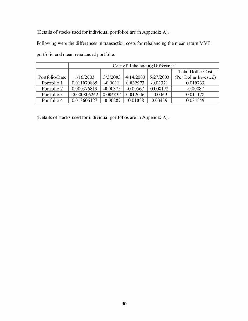
Following were the differences in transaction costs for rebalancing the mean return MVE

portfolio and mean rebalanced portfolio.

Cost of Rebalancing Difference

Portfolio\Date 1/16/2003 3/3/2003 4/14/2003 5/27/2003Total Dollar Cost

(Per Dollar Invested) Portfolio 1 0.011070865 -0.0011 0.032973 -0.02321 0.019733 Portfolio 2 0.000376819 -0.00375 -0.00567 0.008172 -0.00087 Portfolio 3 -0.000806262 0.006837 0.012046 -0.0069 0.011178 Portfolio 4 0.013606127 -0.00287 -0.01058 0.03439 0.034549

(Details of stocks used for individual portfolios are in Appendix A).

30