an ejection chain algorithm for the quadratic assignment algorithm

An Ejection Chain Algorithm for the QuadraticAssignment Problem

Cesar RegoSchool of Business Administration, University of Mississippi, University, Mississippi 38677

Tabitha JamesDepartment of Business Information Technology, Pamplin College of Business, Virginia Polytechnic Institute andState University, Blacksburg, Virginia 24061

Fred GloverUniversity of Colorado, Boulder, Colorado 80309-0419

In this study, we present a new tabu search algorithmfor the quadratic assignment problem (QAP) that uti-lizes an embedded neighborhood construction called anejection chain. Our ejection chain approach providesa combinatorial leverage effect, where the size of theneighborhood grows multiplicatively while the effort offinding a best move in the neighborhood grows onlyadditively. Our results illustrate that significant improve-ment in solution quality is obtained in comparison tothe traditional swap neighborhood. We also developtwo multistart tabu search algorithms utilizing the ejec-tion chain approach in order to demonstrate the powerof embedding this neighborhood construction within amore sophisticated heuristic framework. Comparisons tothe best large neighborhood approaches from the litera-ture are presented. © 2009 Wiley Periodicals, Inc. NETWORKS,Vol. 00(00), 000–000 2010

Keywords: ejection chains; tabu search; combinatorial optimiza-tion; quadratic assignment problem

1. INTRODUCTION

The quadratic assignment problem (QAP) is a classicalcombinatorial optimization problem that has garnered muchattention due to both its large number of applications andits solution complexity. Originally used to model a loca-tion problem in the 1950’s [37], the QAP is computationallyvery difficult to solve which makes it an ideal candidate fortesting new algorithmic approaches. While facility location

Received September 2007; accepted August 2009Correspondence to: C. Rego; e-mail: [email protected] 10.1002/net.20360Published online in Wiley InterScience (www.interscience.wiley.com).© 2009 Wiley Periodicals, Inc.

problems remain the most popular application area for thequadratic assignment problem, many other applications forthis problem exist including scheduling problems, statisticaldata analysis, information retrieval, as well as problems intransportation. The attractiveness of the QAP is also due tothe fact that many other combinatorial optimization problemscan be formulated as a QAP, including the traveling salesmanproblem, the maximum clique problem and the graph parti-tioning problem. (See [6] for a survey of both classical andpractical applications.)

In the context of facility location problems, the QAP can bestated as follows. Let F = {f1, . . . , fn} be a set of n facilitiesto be placed in exactly n locations represented by the setL = {l1, . . . , ln}. A = (aik) is a matrix of distances betweenpairs of locations li, lk ∈ L, and B = (bjl) is an associatedmatrix of flows to be transmitted (or shipped) between pairsof facilities fj, fl ∈ F. The objective is to find a minimumcost assignment of facilities to locations considering both theflow of materials between facilities and the distance betweenlocations.

In mathematical terms, each assignment can be defined asa permutation π of the underlying index set N = {1, . . . , n},i.e. π : N → N . Hence, if facility j is assigned to locationi and facility l is assigned to location k, the cost of the flowbetween facilities j = π(i) and l = π(k) is aikbπ(i)π(k). Theobjective of the QAP is to find a permutation vector π ∈ �n

that minimizes the total assignment cost, where �n is the setof all possible permutations of N. Such a formulation can begenerically described as

Minimizeπ∈ �n

n∑i=1

n∑j=1

aijbπ(i)π(j).

Heuristic approaches for the QAP abound in the literaturewherein local search is commonly used as a basic component

NETWORKS—2010—DOI 10.1002/net

to explore the solution space. Among these heuristics aretabu search [22, 33], scatter search [7], genetic algorithms[2,8,9,13,22,24], ant colony optimization [31], GRASP [20],GRASP with path relinking [25], and path relinking [19].

Local search methods rely on the exploration of a definedneighborhood to generate moves in the solution space ofthe problem under consideration. In the case of the QAP,this neighborhood is typically a 2-exchange neighborhoodthat swaps the location of two facilities at each step of thelocal search process. The exploration of larger neighborhoodswhere the simultaneous movement of k nodes of the permu-tation can be examined is attractive though computationallyvery demanding.

Ahuja et al. [1] introduce a very large scale neighborhoodsearch (VLSN) method for the QAP, which constitutes animportant advance in the creation of more complex neighbor-hoods for the problem. This algorithm iteratively examinesall paths (or exchanges of nodes) of increasing depth, wherethe maximum depth is a specified parameter. The VLSN algo-rithm considers all moves (or a defined subset of moves) ofa given depth before proceeding to the next depth. Becauseof the computational complexity of the full path enumera-tion scheme presented, a maximum path length of k = 4 wassettled upon in their study.

Ejection chain methods constitute a special class of verylarge neighborhoods that have proved highly promising in thesolution of difficult and large scale combinatorial optimiza-tion problems. In general, ejection chains provide the abilityto strategically extend simpler neighborhoods, such as thoseconsisting of exchange (swap) moves or insert (shift) moves,to create more complex neighborhoods that can be generatedwith an efficient investment of effort [16]. Some forms ofejection chain methods make use of a reference structure as aframework for generating moves at each level of the ejectionchain construction [17, 18].

Examples of successful applications of various types ofejection chains include: the multinode insertion and exchangeejection chain method for the classical vehicle routing prob-lem [28], the long-chain shift neighborhood for the general-ized assignment problem [36], the stem-and-cycle (S&C),and the doubly-rooted S&C reference structures for thetraveling salesman problem [26, 29], the flower referencestructure for the vehicle routing problem [27], and the sub-graph ejection chain method for the crew scheduling problem[4].

The key contribution of this article is the development ofa specialized ejection chain algorithm for the QAP, drawingon a proposal sketched in Ref. [16], which has useful featuresin the QAP setting. The approach utilizes the ejection chainstructure to build successively larger exchanges based uponthe elements chosen in the proceeding chain. In this manner,only a selected subset of all possible chains at each depth isconsidered for a given permutation. This process allows themethod to quickly probe larger neighborhoods, with no con-straints on the depths examined, by constructing these chainsof moves based upon previously promising structures. Moreimportantly, these ejection chain neighborhoods exhibit a

special property called combinatorial leverage, where a levelk neighborhood contains O(nk) elements, but a potentiallybest member for a k-neighborhood (k > 2) is determinedwith k examinations of O(n) “component” elements.

We embed our ejection chain method within a tabu search(TS) framework to provide strategic control over the forma-tion of the chains. The first version of our TS method isextremely simple, using memory only in the role of “book-keeping” operations instead of in the role of performingadvanced guidance. Our chief purpose in examining thissimple structure is to show that the ejection chain neighbor-hood obtains better solutions than an exchange neighborhoodin the same framework. We then extend this basic frame-work to present two multistart tabu search variants that yieldsolutions of higher quality and demonstrate the advantagesof embedding ejection chains within a more sophisticatedmetaheuristic. We also provide computational comparisonsto previous large neighborhood approaches.

2. THE EJECTION CHAIN METHOD

Our ejection chain method extends the classical 2-exchange (or swap) neighborhood for the QAP to effectivelycreate more general k-exchange neighborhoods where k cantake any integer value between 2 and n. The method maybe conceived as providing a variable depth neighborhoodthat determines the value of k dynamically according to thecurrent state of the search.

Underlying a general ejection chain design, exchangemoves are successively embedded in the ejection chain con-struction, level by level, and are driven by the evaluationof two types of interrelated moves: (1) an ejection move,which extends the depth of the neighborhood by generatingan intermediate (reference) structure; and (2) a trial move,which creates a feasible solution from the intermediate struc-ture provided by the ejection move. The structure obtainedwith the application of the trial move is called a trial solution.

Our QAP ejection chain method constitutes a node-basedejection chain model where facilities are associated withnodes in a graph which are to be assigned to locations. In thiscontext the method implements a type of multinode exchangemove, which can be seen as a series of swap moves for theQAP.

2.1. The Ejection Chain Neighborhood

We represent a QAP solution as a perfect matching in abipartite graph. Let G = (F ∪ L, F × L) be a (complete)bipartite graph with F = {f1, . . . , fn} representing facilitiesand L = {l1, . . . , ln} representing locations. A solution forthe QAP can be defined by a partial graph S = (F ∪ L, E ⊂F ×L) such that (fi, lj) ∈ E if and only if facility fi is assignedto location lj and no two arcs are incident to the same node.

An ejection chain neighborhood can be definedon a subgraph H = (W , T) of S where T ={(f 0, l0), . . . , (f k , lk), . . . (f l, ll)} is a set of arcs represent-ing l + 1 levels of an ejection chain, which we denote by

2 NETWORKS—2010—DOI 10.1002/net

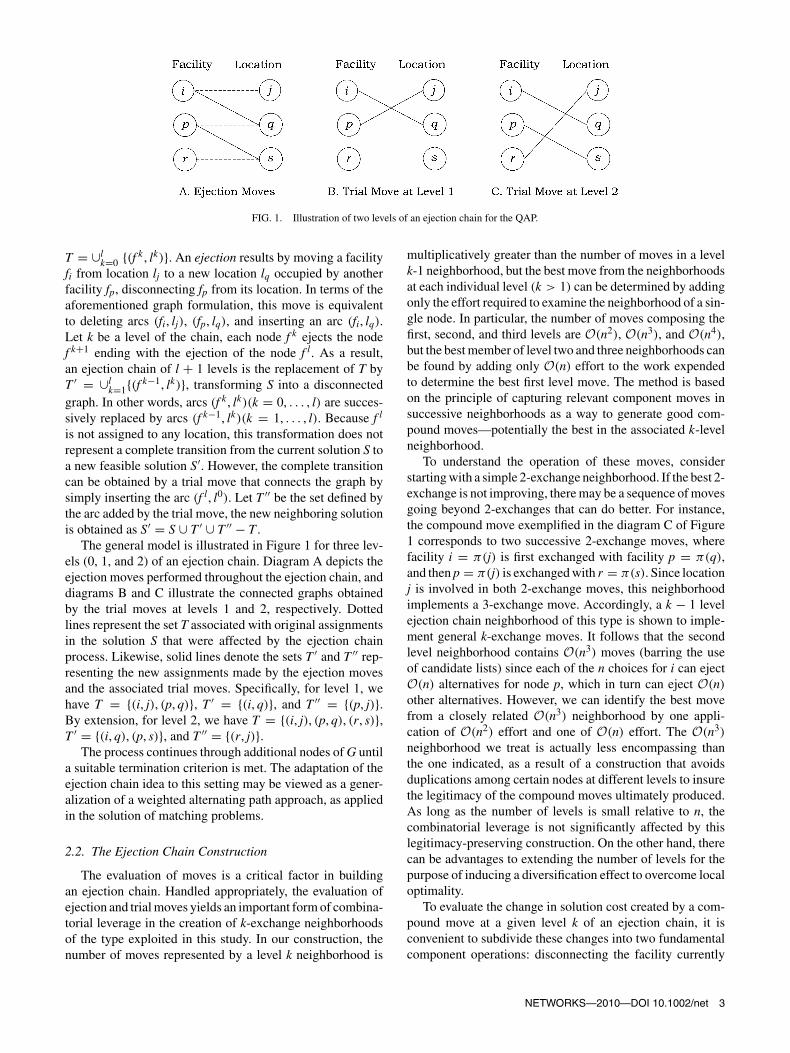
FIG. 1. Illustration of two levels of an ejection chain for the QAP.

T = ∪lk=0 {(f k , lk)}. An ejection results by moving a facility

fi from location lj to a new location lq occupied by anotherfacility fp, disconnecting fp from its location. In terms of theaforementioned graph formulation, this move is equivalentto deleting arcs (fi, lj), (fp, lq), and inserting an arc (fi, lq).Let k be a level of the chain, each node f k ejects the nodef k+1 ending with the ejection of the node f l. As a result,an ejection chain of l + 1 levels is the replacement of T byT ′ = ∪l

k=1{(f k−1, lk)}, transforming S into a disconnectedgraph. In other words, arcs (f k , lk)(k = 0, . . . , l) are succes-sively replaced by arcs (f k−1, lk)(k = 1, . . . , l). Because f l

is not assigned to any location, this transformation does notrepresent a complete transition from the current solution S toa new feasible solution S′. However, the complete transitioncan be obtained by a trial move that connects the graph bysimply inserting the arc (f l, l0). Let T ′′ be the set defined bythe arc added by the trial move, the new neighboring solutionis obtained as S′ = S ∪ T ′ ∪ T ′′ − T .

The general model is illustrated in Figure 1 for three lev-els (0, 1, and 2) of an ejection chain. Diagram A depicts theejection moves performed throughout the ejection chain, anddiagrams B and C illustrate the connected graphs obtainedby the trial moves at levels 1 and 2, respectively. Dottedlines represent the set T associated with original assignmentsin the solution S that were affected by the ejection chainprocess. Likewise, solid lines denote the sets T ′ and T ′′ rep-resenting the new assignments made by the ejection movesand the associated trial moves. Specifically, for level 1, wehave T = {(i, j), (p, q)}, T ′ = {(i, q)}, and T ′′ = {(p, j)}.By extension, for level 2, we have T = {(i, j), (p, q), (r, s)},T ′ = {(i, q), (p, s)}, and T ′′ = {(r, j)}.

The process continues through additional nodes of G untila suitable termination criterion is met. The adaptation of theejection chain idea to this setting may be viewed as a gener-alization of a weighted alternating path approach, as appliedin the solution of matching problems.

2.2. The Ejection Chain Construction

The evaluation of moves is a critical factor in buildingan ejection chain. Handled appropriately, the evaluation ofejection and trial moves yields an important form of combina-torial leverage in the creation of k-exchange neighborhoodsof the type exploited in this study. In our construction, thenumber of moves represented by a level k neighborhood is

multiplicatively greater than the number of moves in a levelk-1 neighborhood, but the best move from the neighborhoodsat each individual level (k > 1) can be determined by addingonly the effort required to examine the neighborhood of a sin-gle node. In particular, the number of moves composing thefirst, second, and third levels are O(n2), O(n3), and O(n4),but the best member of level two and three neighborhoods canbe found by adding only O(n) effort to the work expendedto determine the best first level move. The method is basedon the principle of capturing relevant component moves insuccessive neighborhoods as a way to generate good com-pound moves—potentially the best in the associated k-levelneighborhood.

To understand the operation of these moves, considerstarting with a simple 2-exchange neighborhood. If the best 2-exchange is not improving, there may be a sequence of movesgoing beyond 2-exchanges that can do better. For instance,the compound move exemplified in the diagram C of Figure1 corresponds to two successive 2-exchange moves, wherefacility i = π(j) is first exchanged with facility p = π(q),and then p = π(j) is exchanged with r = π(s). Since locationj is involved in both 2-exchange moves, this neighborhoodimplements a 3-exchange move. Accordingly, a k − 1 levelejection chain neighborhood of this type is shown to imple-ment general k-exchange moves. It follows that the secondlevel neighborhood contains O(n3) moves (barring the useof candidate lists) since each of the n choices for i can ejectO(n) alternatives for node p, which in turn can eject O(n)

other alternatives. However, we can identify the best movefrom a closely related O(n3) neighborhood by one appli-cation of O(n2) effort and one of O(n) effort. The O(n3)

neighborhood we treat is actually less encompassing thanthe one indicated, as a result of a construction that avoidsduplications among certain nodes at different levels to insurethe legitimacy of the compound moves ultimately produced.As long as the number of levels is small relative to n, thecombinatorial leverage is not significantly affected by thislegitimacy-preserving construction. On the other hand, therecan be advantages to extending the number of levels for thepurpose of inducing a diversification effect to overcome localoptimality.

To evaluate the change in solution cost created by a com-pound move at a given level k of an ejection chain, it isconvenient to subdivide these changes into two fundamentalcomponent operations: disconnecting the facility currently

NETWORKS—2010—DOI 10.1002/net 3

assigned to location j, and relocating facility i to location j.Denote the first ejected node (which initiates the chain) bythe top node t, and the current ejected node by the bottomnode b. We let π(i) represent the facility at location i in asolution corresponding to a trial ejection chain under con-sideration, and π ′(i) represent the facility at location i in acurrent solution.

Because the selection of the initial top and bottom nodesrequires the evaluation of the trial move that is made afterejecting the potential bottom node, the relocation of the bot-tom node into the position vacated by the top node must beevaluated before relocating the top node. This particularitymakes the relocation operation at the first level of the ejectionchain different from the relocations used in the ejection andtrial moves performed at higher levels of the chain (where therelocation of the current bottom node is evaluated after thebottom node at the previous level already occupies its newposition).

For this reason, it is convenient to define a special reloca-tion operation aimed at circularizing the ejection move at thefirst level of the ejection chain. The cost changes associatedwith these operations may be expressed as follows:

Disconnection value: D(j) = −n∑

h=1

ahjbπ(h)π(j) h �= j, t

Relocation value: R(i, j) =n∑

h=1

ajhbiπ(h) h �= j, t

Circularization value: C(j) =

⎧⎪⎪⎪⎪⎨⎪⎪⎪⎪⎩

n∑h=1

athbπ(j)π(h) h �= j, t

n∑h=1

athbπ(t)π(h) h = j, h �= t

Hence, for the symmetric QAP, the actual solution costchange associated with these operations is twice the valueobtained by the corresponding operation. The generalizationof these operations to the asymmetric variant of the problemcan be obtained by simply creating additional product termsthat switch the indexes of the product terms above and addingthese new terms to the preceding expressions.

Let ejection value denote the solution cost change asso-ciated with the ejection moves, and let trial value denotethe solution cost change associated with a trial move. Then,an ejection chain of l levels satisfying the requirements oflegitimacy may be recursively evaluated as follows:

Ejection value:

E(k) ={D(t) + D(bk) + R(π(t), bk) k = 1E(k − 1) + D(bk) + R(π ′(bk−1), bk) 1 < k ≤ l

Trial value: �(k) ={E(k) + C(bk) k = 1E(k) + R(π ′(bk), t) 1 < k ≤ l

Letting Z(S) be the cost of the current QAP solution S, thevalue of a trial solution Sk obtained at a level k of the ejection

chain is given by Z(Sk) = Z(S) + 2�(k) for the symmetriccase. As previously mentioned, for the asymmetric case, thelast term would include the reverse products in D, R, andC rather than being doubled. The method keeps track of thelevel k∗ where the best trial solution has been found, whichcorresponds to the depth of the compound move applied tothe current solution S so as to obtain the new neighboringsolution S′. Figure 2 gives an example of these calculations forthe evaluation of two levels of an ejection chain. To simplifythe illustration and keep the equations short, the exampleconsiders the symmetric QAP and assumes that the transitionto a new neighboring solution is performed at level two.

In the illustration, the chain starts with t = 2 and b1 = 3as the initial top and bottom nodes, respectively. The firstoperations consist of disconnecting these two nodes from thegraph and relocating (facility) node 2 in the location previ-ously occupied by node 3, keeping node 2 disconnected. Thealgebraic sum of these three operations gives the value of theejection move E(1) for the first level of the chain. The valueof the trial move �(1) associated with the current ejectionis obtained by circularizing the chain, relocating the currentejected node 3 to occupy the location vacated by the top node2. At this point, the value of the corresponding trial solutionZ(S1) can be calculated by adding the circularization valueto the value of the starting solution. The second level is cre-ated by choosing facility 1 at location 4 to be ejected by thecurrently disconnected (bottom) node b1 = 3, thus settingb2 = 4. The new ejection value is then computed by addingthe disconnection and relocation values D(4) and R(3, 4) ofthe current ejection to the previously obtained ejection valueE(1). Finally, the new trial value �(2) is obtained by addingthe relocation value of facility 1 into the original position ofthe top node to the current ejection value.

2.3. The Ejection Chain Procedure

The ejection chain method begins by identifying the bestlocal move for each facility j, which constitutes removing jfrom its current location and relocating it in the position occu-pied by a facility l, which is thereby ejected. (The method canalso start by looking at each l and finding the best j to replaceit.) The first level of the ejection chain consists of selectinginitial chains based on performing a series of best 2-exchangemoves. Notably, such a move corresponds to simultaneouslydetermining the best initial node to be ejected and the bestnode to occupy the location of the ejected node. The chaingrows by selecting a new node to be ejected by the previouslyejected node. Under the natural restriction that prevents anelement from being moved twice, the chain can continue togrow until all n nodes have been ejected. The pseudocode forthe ejection chain procedure is sketched in Figure 3.

3. TABU SEARCH ALGORITHMS

Rudimentary tabu search (TS) approaches of the typeconsidered here employ short term memory structures to for-bid moves that lead to solutions recently visited (rendering


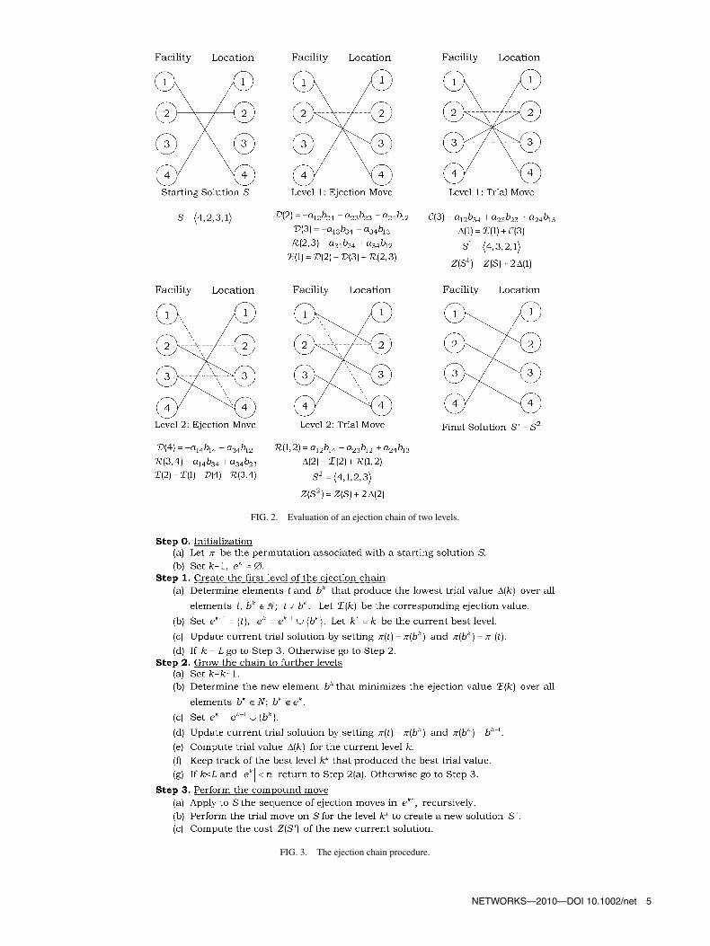
FIG. 2. Evaluation of an ejection chain of two levels.

FIG. 3. The ejection chain procedure.


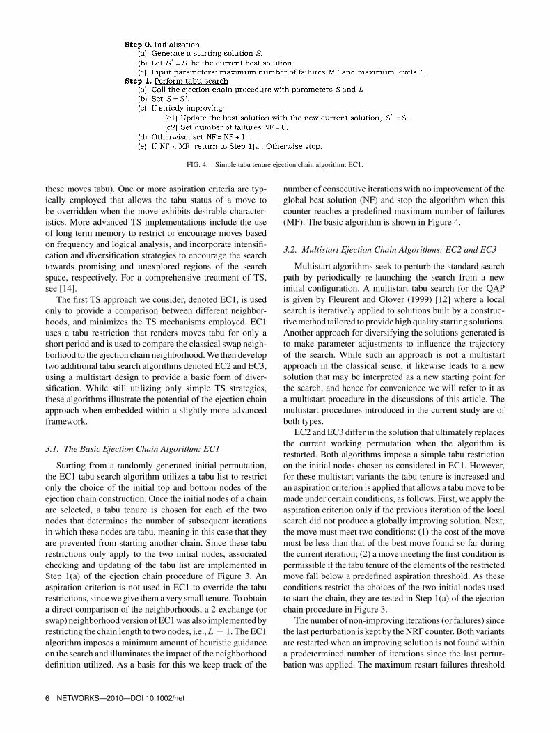
FIG. 4. Simple tabu tenure ejection chain algorithm: EC1.

these moves tabu). One or more aspiration criteria are typ-ically employed that allows the tabu status of a move tobe overridden when the move exhibits desirable character-istics. More advanced TS implementations include the useof long term memory to restrict or encourage moves basedon frequency and logical analysis, and incorporate intensifi-cation and diversification strategies to encourage the searchtowards promising and unexplored regions of the searchspace, respectively. For a comprehensive treatment of TS,see [14].

The first TS approach we consider, denoted EC1, is usedonly to provide a comparison between different neighbor-hoods, and minimizes the TS mechanisms employed. EC1uses a tabu restriction that renders moves tabu for only ashort period and is used to compare the classical swap neigh-borhood to the ejection chain neighborhood. We then developtwo additional tabu search algorithms denoted EC2 and EC3,using a multistart design to provide a basic form of diver-sification. While still utilizing only simple TS strategies,these algorithms illustrate the potential of the ejection chainapproach when embedded within a slightly more advancedframework.

3.1. The Basic Ejection Chain Algorithm: EC1

Starting from a randomly generated initial permutation,the EC1 tabu search algorithm utilizes a tabu list to restrictonly the choice of the initial top and bottom nodes of theejection chain construction. Once the initial nodes of a chainare selected, a tabu tenure is chosen for each of the twonodes that determines the number of subsequent iterationsin which these nodes are tabu, meaning in this case that theyare prevented from starting another chain. Since these taburestrictions only apply to the two initial nodes, associatedchecking and updating of the tabu list are implemented inStep 1(a) of the ejection chain procedure of Figure 3. Anaspiration criterion is not used in EC1 to override the taburestrictions, since we give them a very small tenure. To obtaina direct comparison of the neighborhoods, a 2-exchange (orswap) neighborhood version of EC1 was also implemented byrestricting the chain length to two nodes, i.e., L = 1. The EC1algorithm imposes a minimum amount of heuristic guidanceon the search and illuminates the impact of the neighborhooddefinition utilized. As a basis for this we keep track of the

number of consecutive iterations with no improvement of theglobal best solution (NF) and stop the algorithm when thiscounter reaches a predefined maximum number of failures(MF). The basic algorithm is shown in Figure 4.

3.2. Multistart Ejection Chain Algorithms: EC2 and EC3

Multistart algorithms seek to perturb the standard searchpath by periodically re-launching the search from a newinitial configuration. A multistart tabu search for the QAPis given by Fleurent and Glover (1999) [12] where a localsearch is iteratively applied to solutions built by a construc-tive method tailored to provide high quality starting solutions.Another approach for diversifying the solutions generated isto make parameter adjustments to influence the trajectoryof the search. While such an approach is not a multistartapproach in the classical sense, it likewise leads to a newsolution that may be interpreted as a new starting point forthe search, and hence for convenience we will refer to it asa multistart procedure in the discussions of this article. Themultistart procedures introduced in the current study are ofboth types.

EC2 and EC3 differ in the solution that ultimately replacesthe current working permutation when the algorithm isrestarted. Both algorithms impose a simple tabu restrictionon the initial nodes chosen as considered in EC1. However,for these multistart variants the tabu tenure is increased andan aspiration criterion is applied that allows a tabu move to bemade under certain conditions, as follows. First, we apply theaspiration criterion only if the previous iteration of the localsearch did not produce a globally improving solution. Next,the move must meet two conditions: (1) the cost of the movemust be less than that of the best move found so far duringthe current iteration; (2) a move meeting the first condition ispermissible if the tabu tenure of the elements of the restrictedmove fall below a predefined aspiration threshold. As theseconditions restrict the choices of the two initial nodes usedto start the chain, they are tested in Step 1(a) of the ejectionchain procedure in Figure 3.

The number of non-improving iterations (or failures) sincethe last perturbation is kept by the NRF counter. Both variantsare restarted when an improving solution is not found withina predetermined number of iterations since the last pertur-bation was applied. The maximum restart failures threshold


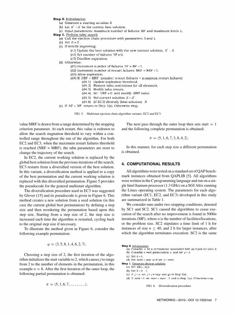
FIG. 5. Multistart ejection chain algorithm variants: EC2 and EC3.

value MRF is drawn from a range determined by the stoppingcriterion parameter. At each restart, this value is redrawn toallow the search stagnation threshold to vary within a con-trolled range throughout the run of the algorithm. For bothEC2 and EC3, when the maximum restart failures thresholdis reached (NRF = MRF), the tabu parameters are reset tochange the trajectory of the search.

In EC2, the current working solution is replaced by theglobal best solution from the previous iterations of the search.EC3 restarts from a diversified version of the best solution.In this variant, a diversification method is applied to a copyof the best permutation and the current working solution isreplaced with this diversified permutation. Figure 5 providesthe pseudocode for the general multistart algorithm.

The diversification procedure used in EC3 was suggestedby Glover [15] and its pseudocode is given in Figure 6. Thismethod creates a new solution from a seed solution (in thiscase the current global best permutation) by defining a stepsize and then reordering the permutation based upon thisstep size. Starting from a step size of 2, the step size isincreased each time the algorithm is restarted, cycling backto the original step size if necessary.

To illustrate the method given in Figure 6, consider thefollowing example permutation:

ϕ = 〈3, 5, 8, 1, 4, 6, 2, 7〉.

Choosing a step size of 2, the first iteration of the algo-rithm initializes the start variable to 2, which causes j to rangefrom 2 to the number of elements in the permutation, in thisexample n = 8. After the first iteration of the outer loop, thefollowing partial permutation is obtained:

π = 〈5, 1, 6, 7, −, −, −, −〉.

The next pass through the outer loop then sets start = 1and the following complete permutation is obtained:

π = 〈5, 1, 6, 7, 3, 8, 4, 2〉.In this manner, for each step size a different permutation

is obtained.

4. COMPUTATIONAL RESULTS

All algorithms were tested on a standard set of QAP bench-mark instances obtained from QAPLIB [5]. All algorithmswere written in the C programming language and run on a sin-gle Intel Itanium processor (1.3 GHz) on a SGI Altix runningthe Linux operating system. The parameters for each algo-rithm variant (EC1, EC2, and EC3) developed in this studyare summarized in Table 1.

We consider runs under two stopping conditions, denotedby SC1 and SC2. SC1 caused the algorithms to cease exe-cution of the search after no improvement is found in 5000niterations (MF), where n is the number of facilities/locations,or the problem size. SC2 stipulates a time limit of 1 h forinstances of size n ≤ 40, and 2 h for larger instances, afterwhich the algorithm terminates execution. SC2 is the same

FIG. 6. Diversification procedure.


TABLE 1. TS Variant parameter settings.

Parameter EC1 EC2 EC3

Maximum failures (MF) (Stopping criterion SC1) 5000n 5000n 5000nTime limit, h 1 (n ≤ 40) 1 (n ≤ 40) 1 (n ≤ 40)(Stopping criterion SC2) 2 (n > 40) 2 (n > 40) 2 (n > 40)Allowable failures (MRF)Lower limit n/a 5n 5nUpper limit n/a 500n 500n(Restart criterion)Tabu tenureLower limit (LT) 3 (static) n/10 (variable) n/10 (variable)Upper limit (UT) 10 (static) 3n/10 (variable) 3n/10 (variable)Aspiration threshold n/a (LT+UT)/2 (LT+UT)/2Restart tabu tenureLower limit (LT) n/a n/10 n/10Upper limit (UT) n/a n nRestart solution n/a global best diversified global best

stopping condition applied in Ref. [1] and is used to allow fora direct comparison with the associated VLSN algorithms.

Tables 2 and 3 present computational results for allvariants of the algorithms under SC1 and SC2 stopping con-ditions, respectively. The parameters used in all algorithmsfor both Tables 2 and 3 are the same with the exception ofthe stopping condition. All algorithms ran 10 times on eachproblem instance, each time starting from a randomly gener-ated seed solution. The tabu tenure for EC1 was set to be aninteger value randomly drawn from the range 3–10. The tabutenure for EC2 and EC3 is initialized with a value chosenfrom the range n/10 and 3n/10. At each restart for EC2 andEC3, the tabu search parameters are adjusted. The upper andlower limits, that are used to determine the tabu tenure for anelement are redrawn and allowed to vary in the range n/10 ton. Similarly, the maximum restart failures (MRF) parameteris reset every time a restart occurs for both the EC2 and EC3variants. At each restart MRF is chosen from the range 5n to500n. As previously mentioned no aspiration criterion is usedin EC1, while for EC2 and EC3 tabu active moves are sub-jected to two aspiration conditions. In our implementation,the required aspiration threshold is defined to be the aver-age of the lower and upper limits of the current tabu tenurerange. Also, as remarked EC2 and EC3 algorithms differ inthe mechanism used to restart the search: EC2 restarting fromthe current global best solution, and EC3 restarting from adiversified version of the global best solution.

Table 2 and Table 3 follow the same format. The first twocolumns provide the name of the test instance and the corre-sponding best known solution (BKS). The next columns areorganized in four groups associated with each variant of ourejection chain algorithm. The first two groups represent thesimple tabu search algorithm restricted to first-level ejectionchains to implement a 2-exchange neighborhood (2-exchangeEC1), and its extension to n-level ejection chains implement-ing a variable depth k-exchange neighborhood (EC1). Thenext two groups correspond to the two multistart tabu searchvariants using either the current global best solution (EC2) ora diversified version of it (EC3) as a perturbation scheme to

restart the search. For each algorithm we provide the averagepercent deviation (APD) to the BKS, the best percent devi-ation (BPD) for only the best solution obtained from the 10runs, the average iteration the best solution was found (ABI),and either the average running time to completion (ATTC) inminutes using stopping criterion SC1 (Table 2) or the aver-age running time to solution (ATTS) using stopping criterionSC2 (Table 3).

Figure 7 graphically depicts the average solution qualityof the three EC variants and the 2-exchange neighborhoodfrom Table 2. Figure 8 shows a comparison of the averagetimes to completion for all algorithms in Table 2 on eachproblem instance.

Table 2 shows that the ejection chain neighborhoodimproved the average solution quality of all but 4 problemsover the 2-exchange neighborhood embedded in the sameheuristic. The impact of the ejection chain neighborhood canbe easily observed as EC1 obtained better average results thanthe 2-exchange EC1 algorithm on 19 of the 22 test problemsand tied on 1. The 2-exchange EC1 and EC1 are identicalalgorithms except for the neighborhood utilized. In the 2-exchange EC1 algorithm, the maximum length of the chainwas limited to 2 nodes, which simulates a 2-exchange neigh-borhood. The best overall solution was found by EC1 for 12of the 22 problems, with the 2-exchange version obtaining thebest overall solution for 9 of 22, with a tie for one problemwhere both variants found the BKS.

In Table 3 the results were similar. EC1 using the ejectionchain neighborhood obtained better average results on 13 ofthe 22 problem instances and tied on 1. The performancewas degraded a small amount due to the time limit imposed.It should be noted that the 2-exchange neighborhood algo-rithm is able to perform around twice as many iterations inthe same amount of time as the ejection chain neighborhood.While the ejection chain neighborhood is quick compared toa full k-opt exploration, it is still slower than a swap neigh-borhood. This leads to an interesting observation. In Table 3,where the runtime of the algorithm was restricted, the ejec-tion chain neighborhood still outperformed the 2-exchange


TAB

LE

2.C

ompu

tatio

nalr

esul

tsfo

rSk

orin

–Kap

ovpr

oble

ms

and

sym

met

ric

Taill

ard

prob

lem

sus

ing

stop

ping

crite

rion

1.

2-O

ptE

C1

EC

1E

C2

EC

3

Prob

lem

BK

SA

PDB

PDA

BI

AT

TC

APD

BPD

AB

IA

TT

CA

PDB

PDA

BI

AT

TC

APD

BPD

AB

IA

TT

C

Skor

in–K

apov

inst

ance

ssk

o42

1581

20.

120

0.00

012

1327

2.46

0.02

80.

000

1410

034.

780.

293

0.00

012

7261

6.16

0.06

10.

000

1811

447.

15sk

o49

2338

60.

199

0.05

181

096

4.51

0.19

90.

000

5682

17.

050.

235

0.05

110

5762

11.0

00.

086

0.05

116

4692

13.0

2sk

o56

3445

80.

418

0.01

210

1949

8.70

0.52

70.

075

6994

412

.78

0.47

50.

012

2048

4222

.96

0.25

90.

029

1448

4119

.97

sko6

448

498

0.64

40.

107

1455

3819

.66

0.46

40.

000

8641

127

.64

0.24

30.

008

2713

4250

.46

0.13

90.

000

3305

8455

.50

sko7

266

256

0.93

20.

211

2113

6534

.30

0.69

10.

072

2241

7954

.37

0.32

20.

060

2524

8369

.86

0.34

00.

211

3105

6776

.20

sko8

190

998

0.90

10.

090

2176

8758

.79

0.84

90.

259

7656

770

.54

0.33

60.

097

2992

7512

1.94

0.27

10.

044

3785

4313

6.34

sko9

011

5534

0.69

10.

230

2542

7997

.54

0.88

10.

389

1043

9511

7.12

0.30

50.

000

5878

2925

6.00

0.27

20.

014

4435

3921

9.75

sko1

00a

1520

020.

736

0.37

822

5563

146.

470.

661

0.40

418

2165

213.

580.

314

0.02

644

4283

334.

820.

263

0.13

345

1170

337.

15sk

o100

b15

3890

0.86

80.

659

1764

4513

6.42

0.80

30.

298

3380

3726

2.14

0.37

90.

127

3792

7331

1.93

0.22

60.

087

3780

5131

1.29

sko1

00c

1478

621.

108

0.55

725

6918

152.

550.

779

0.17

017

6688

211.

840.

731

0.03

061

6575

396.

260.

269

0.10

747

0522

344.

28sk

o100

d14

9576

1.00

70.

389

5919

911

2.66

0.86

20.

594

1064

2218

9.76

0.43

70.

070

3690

6730

7.84

0.31

60.

060

6676

5641

4.04

sko1

00e

1491

501.

178

0.80

136

3182

174.

001.

147

0.61

518

8224

215.

460.

522

0.02

042

8918

329.

180.

198

0.02

058

3862

384.

48sk

o100

f14

9036

0.98

90.

769

3244

6316

6.58

0.97

90.

498

7679

618

0.70

0.56

70.

169

4680

7534

4.04

0.39

50.

203

4121

3432

3.81

Ave

rage

0.75

30.

327

1953

0885

.74

0.62

80.

260

1405

8912

0.60

0.39

70.

052

3503

8319

7.11

0.23

80.

074

3782

5420

3.31

Sym

met

ric

Taill

ard

inst

ance

sta

i20a

1224

5531

90.

906

0.00

070

967

0.38

0.71

80.

304

6080

50.

310.

152

0.00

066

085

0.22

0.19

90.

000

5030

30.

20ta

i25a

3443

5564

61.

523

0.93

710

9665

0.23

0.67

00.

000

6324

50.

270.

294

0.00

061

480

0.71

0.05

50.

000

7638

80.

69ta

i30a

6371

1711

30.

959

0.39

814

4811

0.45

0.64

50.

490

1275

721.

290.

178

0.00

071

869

1.60

0.13

70.

000

6131

11.

29ta

i35a

2833

1544

51.

123

0.59

514

3038

1.08

0.97

20.

698

9811

71.

920.

302

0.00

014

3831

3.29

0.27

20.

000

1511

373.

38ta

i40a

6372

5094

81.

022

0.43

917

2807

2.19

0.82

50.

416

2025

774.

500.

420

0.30

513

9842

5.38

0.38

70.

120

1834

526.

10ta

i50a

4588

2151

71.

090

0.71

021

2317

6.67

1.05

80.

721

1982

3511

.14

0.73

20.

572

1695

7213

.81

0.72

60.

564

1897

0914

.30

tai6

0a60

8215

054

1.02

50.

775

2304

8516

.99

1.01

70.

602

1577

5523

.78

0.71

50.

499

3085

1540

.43

0.86

10.

601

1340

4728

.60

tai8

0a81

8415

043

0.80

40.

625

3246

3864

.78

0.69

50.

453

3113

1397

.93

0.64

40.

392

4652

7114

2.07

0.78

00.

581

2117

6010

0.09

tai1

00a

1185

9961

370.

481

0.34

849

1175

200.

140.

563

0.31

130

4380

252.

100.

600

0.27

233

2753

295.

570.

654

0.41

932

1325

291.

44A

vera

ge0.

993

0.53

621

1100

32.5

50.

796

0.44

416

9333

43.6

90.

449

0.22

719

5469

55.9

00.

452

0.25

415

3270

49.5

6O

vera

ll0.

851

0.41

320

1796

63.9

80.

729

0.33

515

2348

89.1

30.

418

0.12

328

7009

139.

340.

326

0.14

728

6215

140.

41

The

best

aver

age

perc

entd

evia

tion

over

alla

lgor

ithm

sis

show

nin

bold

face

.


TAB

LE

3.C

ompu

tatio

nalr

esul

tsfo

rSk

orin

–Kap

ovpr

oble

ms

and

sym

met

ric

Taill

ard

prob

lem

sus

ing

stop

ping

crite

rion

2.

2-O

ptE

C1

EC

1E

C2

EC

3

Prob

lem

BK

SA

PDB

PDA

BI

AT

TS

APD

BPD

AB

IA

TT

SA

PDB

PDA

BI

AT

TS

APD

BPD

AB

IA

TT

S

Skor

in–K

apov

inst

ance

ssk

o42

1581

20.

008

0.00

075

3938

6.61

0.00

00.

000

1034

671.

620.

019

0.00

011

8388

627

.50

0.00

00.

000

9840

1921

.43

sko4

923

386

0.05

30.

000

1888

633

26.8

10.

063

0.00

061

5169

15.0

80.

107

0.05

185

7422

28.0

00.

039

0.00

015

5112

1350

.91

sko5

634

458

0.18

30.

000

1651

179

37.4

80.

324

0.18

611

2798

043

.41

0.30

50.

012

7712

6538

.07

0.02

70.

012

1176

507

58.0

2sk

o64

4849

80.

475

0.09

111

0645

651

.18

0.39

70.

000

5041

5538

.14

0.13

90.

008

4698

2544

.27

0.07

80.

000

6427

9160

.99

sko7

266

256

0.82

70.

211

4733

0630

.55

0.70

50.

196

5934

9160

.92

0.31

90.

060

3169

1939

.52

0.25

00.

115

6352

2479

.22

sko8

190

998

0.85

50.

086

4732

5550

.74

0.94

30.

481

2476

9141

.69

0.36

40.

097

3270

1965

.44

0.27

80.

114

3405

2968

.06

sko9

011

5534

0.69

10.

230

2542

7940

.27

0.78

50.

533

2121

6651

.87

0.42

40.

029

2725

4377

.96

0.47

30.

132

2022

5957

.84

sko1

00a

1520

020.

739

0.37

814

4780

33.4

70.

617

0.16

311

0996

39.9

40.

424

0.11

220

8584

86.1

30.

340

0.19

717

1948

70.8

6sk

o100

b15

3890

0.86

80.

659

1764

4540

.82

0.52

10.

396

9230

433

.19

0.43

60.

149

2388

8898

.71

0.40

80.

140

1299

1253

.54

sko1

00c

1478

621.

122

0.55

716

7928

38.8

21.

445

0.88

913

2206

42.4

80.

963

0.12

718

2385

75.5

30.

543

0.17

218

8109

77.6

3sk

o100

d14

9576

1.00

70.

389

5919

913

.68

1.01

90.

784

1102

9239

.52

0.53

70.

119

2025

6483

.66

0.51

70.

182

2003

0488

.14

sko1

00e

1491

501.

191

0.80

120

2636

46.9

30.

796

0.41

310

1984

36.6

60.

692

0.02

021

6867

89.6

70.

460

0.02

021

4302

88.3

3sk

o100

f14

9036

1.00

80.

782

2373

9152

.01

1.06

30.

625

1006

4836

.20

0.62

70.

279

1872

2777

.53

0.54

20.

421

2038

0884

.19

Ave

rage

0.69

40.

322

5838

0236

.10

0.66

80.

359

3117

3436

.98

0.41

20.

082

4181

0764

.00

0.30

40.

116

5108

4066

.09

Sym

met

ric

Taill

ard

inst

ance

sta

i20a

1224

5531

90.

000

0.00

018

8852

847.

520.

000

0.00

053

5941

25.

800.

000

0.00

041

0389

0.89

0.00

00.

000

2601

520.

56ta

i25a

3443

5564

60.

102

0.00

024

8622

2426

.19

0.00

00.

000

3924

530

9.26

0.00

00.

000

2654

011.

100.

000

0.00

013

2537

0.55

tai3

0a63

7117

113

0.40

20.

016

1056

7411

22.5

80.

161

0.00

063

6737

527

.75

0.00

00.

000

5204

513.

620.

000

0.00

029

3665

2.04

tai3

5a28

3315

445

0.47

90.

082

4647

443

17.6

80.

366

0.06

739

0229

828

.46

0.00

00.

000

5074

355.

510.

000

0.00

091

5365

9.95

tai4

0a63

7250

948

0.51

90.

074

5101

524

31.4

20.

550

0.07

425

4514

128

.88

0.27

40.

074

1728

563

27.7

60.

219

0.07

417

4227

728

.01

tai5

0a45

8821

517

0.80

20.

635

2988

029

44.2

90.

753

0.53

422

0948

656

.93

0.55

00.

352

1045

558

35.5

70.

514

0.36

410

4169

835

.43

tai6

0a60

8215

054

0.88

30.

769

1596

279

54.5

00.

791

0.40

380

0025

45.5

20.

629

0.49

968

5710

49.2

50.

657

0.33

668

5735

49.2

4ta

i80a

8184

1504

30.

745

0.55

953

5781

54.0

10.

714

0.53

241

7335

65.7

10.

681

0.55

442

1467

79.4

60.

730

0.48

634

5948

65.0

5ta

i100

a11

8599

6137

0.56

70.

354

2922

2867

.46

0.55

80.

313

1606

1157

.79

0.71

40.

630

1805

2274

.65

0.72

90.

419

1318

5154

.36

Ave

rage

0.50

00.

277

7719

578

36.1

80.

433

0.21

428

5402

436

.23

0.31

60.

234

6406

1130

.87

0.31

70.

187

6165

8127

.24

Ove

rall

0.61

50.

303

3502

983

36.1

40.

571

0.30

013

5176

236

.67

0.37

30.

144

5091

3150

.45

0.30

90.

145

5540

9850

.20

The

best

aver

age

perc

entd

evia

tion

over

alla

lgor

ithm

sis

show

nin

bold

face

.


FIG. 7. Average percent deviation (APD) for Skorin–Kapov and symmetricTaillard instances. [Color figure can be viewed in the online issue, which isavailable at www.interscience.wiley.com.]

neighborhood in terms of solution quality. On 8 of the 14test instances where the ejection chain neighborhood tied orbested the 2-exchange neighborhood in Table 3, the aver-age time to the best solution (ATTS) for EC1 was actuallyless than the 2-exchange neighborhood EC1. This indicatesthat the ejection chain neighborhood is able to quickly findhigh quality solutions. This is reinforced by the results inTable 2, which shows that allowed to iterate with stagna-tion as the stopping condition, EC1 using the ejection chainneighborhood performs even better against the 2-exchangeneighborhood EC1. These results are obtained in most caseswithout doubling the computational time of the 2-exchangeneighborhood EC1.

In Table 2, as well as in Table 3, the EC3 multistart variantproduced the best overall results of all approaches, obtainingthe best average solution quality for 16 of 22 problems inTable 2. In Table 3, EC3 obtained the best average solutionquality for 14 of 22 problems. However, EC2 and EC3 tiedon 4 of the 22 problems, so the results indicate that EC3 doesas well as or better than all other variants under SC2 on 18of the 22 problems. EC2 had 4 of the best average percentdeviations in Table 2 (3 of 22 in Table 3). EC1 and the 2-exchange EC1 provided one best average percent deviationeach in Table 2. In Table 3, the 2-exchange EC1 obtainedthe best average percent deviation to one problem. The EC2variant, which replaced the current working solution with theglobal best solution rather than a diversified solution, wasclearly outperformed by the EC3 variant. This suggests thatthe use of strategic diversification is highly beneficial andagrees with previous findings where metaheuristics appliedto the QAP that employ some type of diversity have providedgood results [9, 22, 24].

EC2 shows a slight edge over EC3 in obtaining the bestoverall solution. EC2 produced the best overall solutions(BPD) for 8 of 22 problems in Table 2 (7 of 22 in Table 3)while EC3 produced 5 of the best overall solutions in Table2 (3 of 22 in Table 3). EC1 produced 1 best overall solution

in both Tables. In Table 3, 2-exchange neighborhood EC1produced 1 best overall solution. On the other 8 instances inTable 2 (10 in Table 3) at least 2 of the variants tied.

4.1. Comparisons with Very-Large Scale NeighborhoodAlgorithms

The VLSN algorithms introduced by Ahuja et al. [1]employ a type of variable depth k-opt neighborhood and aretherefore appropriate for comparison with our EC algorithms.The purpose of this comparison is to investigate the relativeperformance of the ejection chain algorithms in this studyand other large neighborhood algorithms. To clarify the anal-ysis, it is convenient to discuss the fundamentals of VLSNalgorithms and contrast them to the EC algorithms.

A full path enumeration search requires that every k-exchange be explored and can be prohibitively expensiveeven for relatively small values of k. This expense hasseverely limited attempts to use neighborhoods for the QAPmore complex than the swap neighborhood (which results ink = 2). The VLSN algorithms and the ejection chain algo-rithms contribute alternative approaches for exploring largerneighborhoods.

The VLSN algorithms of Ahuja et al. [1] introduce animprovement graph for the QAP together with several vari-ants of a search algorithm utilizing a large neighborhood.The concept of an improvement graph was first introduced byThompson and Orlin (1989) [34] for partitioning problems.For the QAP, it is used to store partial costs for k-exchanges ona permutation. The initial cost of constructing the improve-ment graph is O(n3); however, once created for a permutationit can be updated in O(kn2) time. The improvement graphdoes not contain the full cost of the k-exchange, rather agood approximation. It is especially useful in a path enumer-ation scheme as it allows for relatively quick evaluation ofa large number of neighbors on a single permutation withthe construction of only one improvement graph. If a new

FIG. 8. Average time to completion (ATTC) for Skorin–Kapov and sym-metric Taillard instances. [Color figure can be viewed in the online issue,which is available at www.interscience.wiley.com.]


permutation is introduced, the improvement graph must bereconstructed.

The ejection chain method, in contrast, exploits a selectivesubset of neighbors, which provides a quick investigation of apromising extended neighborhood rather than examining allexchanges at a given depth. This reduces the number of cal-culations necessary, thus speeding the neighborhood searchprocess without the necessity of maintaining a cost matrix.As in the VLSN method a k-level ejection chain does not nec-essarily produce the overall best k-exchange move, rather apotentially good move. Ejection chain strategies are particu-larly amenable to being exploited within an adaptive memoryTS framework, where other operators may also be applied tothe permutation.

The VLSN search algorithms in Ahuja et al. [1] exploreiteratively larger neighborhoods up to a defined k beginningfrom a randomly drawn permutation. Specifically, the VLSNalgorithms explore all exchanges at depth 2, then all (or apruned subset) exchanges at depth 3, followed lastly by the4-exchanges (in implementation, the algorithms are limitedto a depth of 4). In contrast, the ejection chain method discov-ers the best exchange at depth 2, and then iteratively extendsthat 2-exchange up to a depth of n. The method keeps trackof the level k∗ of the chain where the best trial solution wasfound and then applies the associated k-exchange move tothe permutation and the process is repeated. An iterationof the VLSN algorithms ends when the search on the cur-rent permutation is exhausted (a new best solution is foundor no better solution is found after exploring all allowedk-exchanges). Then a new random permutation is drawn, anew improvement graph is constructed and the process isrepeated. When comparing the two methods, the VLSN algo-rithms more nearly resemble a breadth-first search and the ECalgorithms more nearly resemble a depth-first search, thougheach affords the strategic benefit of avoiding the complex-ity of such classical searches while nevertheless uncoveringhigh quality solutions. Future research that combines the twoapproaches would be of interest.

The difference between the VLSN algorithms concernshow many k-exchanges are examined at a given depth. Theauthors propose four VLSN variants. The first is a full pathenumeration where all paths of a given depth are examined.As previously mentioned this process is very costly and wasruled out by the authors as a viable algorithm. The otherthree variants employed “path pruning” techniques to reducethe number of paths examined at each depth. The secondproposed variant, keeps only paths with a negative cost at eachdepth. The authors state that this variant was outperformed intesting by the other variants, so computational results for thisvariant were not provided. In both VLSN variants, for whichresults are presented, a different path pruning technique isemployed to reduce the number of paths examined at eachdepth. We will refer to these two variants as VLSN1 andVLSN2. In VLSN1, the best αn2 paths with the lowest costat one level are carried forward to the next level to build largerexchanges. In implementation, α is set to 1 and the maximumpath length is set to 4. By contrast, VLSN2 excludes all paths

except for the best path for each node. In other words, only theinitial path from each node that has the lowest cost is allowedto proceed to the next depth. VLSN2 also first performed adescent to a local optimum at depth 2 before beginning pathenumeration.

Table 4 provides comparisons between the two VLSNalgorithms (VLSN1 and VLSN2) and the EC algorithms(EC1, EC2, and EC3) developed for this study using thesame stopping criterion (SC2). The results for SC1 are alsoprovided for some supplemental observations. In addition,we provide in Figure 9 a pairwise comparison of the algo-rithms in terms of the number of best solutions produced overall problems. The VLSN algorithms were run using SC2 ona Pentium IV, 2.4 GHz processor and were also written inthe C programming language. SPEC (2000) [30] shows thatthe processor used in the VLSN study is equivalent to (justslightly better than) the processor used in the current study(Intel Itanium, 1.3 GHz). Therefore, the comparisons are asvalid as possible without having algorithms written by thesame programmer and run on the same machine.

As previously discussed, the EC1 algorithms containedvery limited adaptive memory guidance in the form of a sim-ple tabu list with small tabu tenures. A 2-exchange versionof EC1 is provided to examine the impact of the ejectionchain neighborhood. However, since the VLSN study alsoprovided a 2-exchange algorithm, we can compare the impactof the minimal short-term memory guidance in the EC1 vari-ant. Comparing the 2-exchange versions of VLSN and EC1,the VLSN algorithm performs better on the sko* instanceswhile EC1 is better on the tai∗ instances. Overall, there isno significant difference in the performance of the two 2-exchange algorithms, which demonstrates that the tabu listin the EC1 version had little positive impact other than toprevent cycling.

Another interesting observation can be made examiningthe 2-exchange algorithms. The 2-exchange EC1 algorithmdid especially poorly on the sko∗ instances, losing on 11of the 13 instances. This could indicate that the restrictive-ness of the tabu list was especially detrimental for this set ofinstances. Indeed, experimental analysis conducted duringthe tuning of the algorithm parameters showed better results(on average) when smaller tabu tenures are used for the sko∗instances. However, those parameters were not so suitablefor tai∗ instances and we restricted our method to use thesame parameter values for all instances. In contrast, the 2-exchange VLSN revealed significant difficulty on the largertai∗ instances (n ≥ 40), exceeding the best known solutionsvalue by more than 2%. In fact, the difference in the character-istics of the problem instances becomes especially apparentin the larger neighborhoods. This is also seen to be true whenexamining the difference between the variable-depth versionsof VLSN and the EC algorithms.

VLSN1 performs very well on the sko∗ instances. It per-forms better than EC1 and EC2 on all but one or two instancesand completely dominates VLSN2 on the sko∗ test set. In gen-eral the VLSN algorithms tend to perform better on the sko∗instances; however even in that set both EC2 and EC3 perform


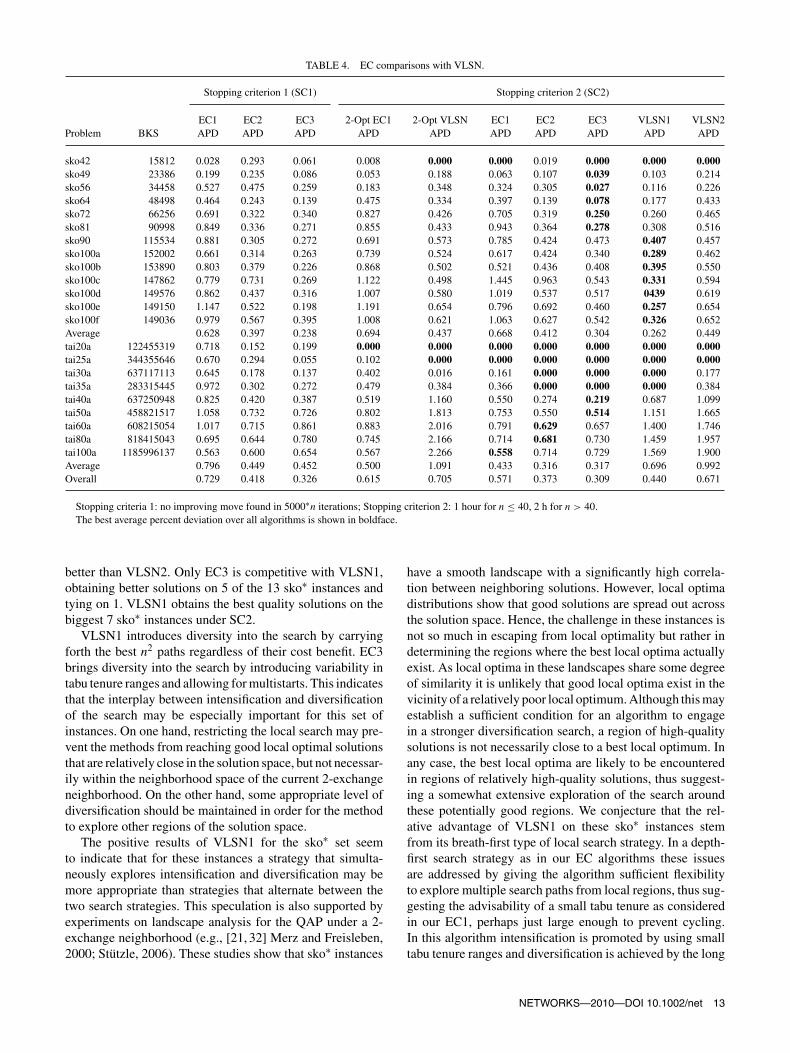
TABLE 4. EC comparisons with VLSN.

Stopping criterion 1 (SC1) Stopping criterion 2 (SC2)

EC1 EC2 EC3 2-Opt EC1 2-Opt VLSN EC1 EC2 EC3 VLSN1 VLSN2Problem BKS APD APD APD APD APD APD APD APD APD APD

sko42 15812 0.028 0.293 0.061 0.008 0.000 0.000 0.019 0.000 0.000 0.000sko49 23386 0.199 0.235 0.086 0.053 0.188 0.063 0.107 0.039 0.103 0.214sko56 34458 0.527 0.475 0.259 0.183 0.348 0.324 0.305 0.027 0.116 0.226sko64 48498 0.464 0.243 0.139 0.475 0.334 0.397 0.139 0.078 0.177 0.433sko72 66256 0.691 0.322 0.340 0.827 0.426 0.705 0.319 0.250 0.260 0.465sko81 90998 0.849 0.336 0.271 0.855 0.433 0.943 0.364 0.278 0.308 0.516sko90 115534 0.881 0.305 0.272 0.691 0.573 0.785 0.424 0.473 0.407 0.457sko100a 152002 0.661 0.314 0.263 0.739 0.524 0.617 0.424 0.340 0.289 0.462sko100b 153890 0.803 0.379 0.226 0.868 0.502 0.521 0.436 0.408 0.395 0.550sko100c 147862 0.779 0.731 0.269 1.122 0.498 1.445 0.963 0.543 0.331 0.594sko100d 149576 0.862 0.437 0.316 1.007 0.580 1.019 0.537 0.517 0439 0.619sko100e 149150 1.147 0.522 0.198 1.191 0.654 0.796 0.692 0.460 0.257 0.654sko100f 149036 0.979 0.567 0.395 1.008 0.621 1.063 0.627 0.542 0.326 0.652Average 0.628 0.397 0.238 0.694 0.437 0.668 0.412 0.304 0.262 0.449tai20a 122455319 0.718 0.152 0.199 0.000 0.000 0.000 0.000 0.000 0.000 0.000tai25a 344355646 0.670 0.294 0.055 0.102 0.000 0.000 0.000 0.000 0.000 0.000tai30a 637117113 0.645 0.178 0.137 0.402 0.016 0.161 0.000 0.000 0.000 0.177tai35a 283315445 0.972 0.302 0.272 0.479 0.384 0.366 0.000 0.000 0.000 0.384tai40a 637250948 0.825 0.420 0.387 0.519 1.160 0.550 0.274 0.219 0.687 1.099tai50a 458821517 1.058 0.732 0.726 0.802 1.813 0.753 0.550 0.514 1.151 1.665tai60a 608215054 1.017 0.715 0.861 0.883 2.016 0.791 0.629 0.657 1.400 1.746tai80a 818415043 0.695 0.644 0.780 0.745 2.166 0.714 0.681 0.730 1.459 1.957tai100a 1185996137 0.563 0.600 0.654 0.567 2.266 0.558 0.714 0.729 1.569 1.900Average 0.796 0.449 0.452 0.500 1.091 0.433 0.316 0.317 0.696 0.992Overall 0.729 0.418 0.326 0.615 0.705 0.571 0.373 0.309 0.440 0.671

Stopping criteria 1: no improving move found in 5000∗n iterations; Stopping criterion 2: 1 hour for n ≤ 40, 2 h for n > 40.The best average percent deviation over all algorithms is shown in boldface.

better than VLSN2. Only EC3 is competitive with VLSN1,obtaining better solutions on 5 of the 13 sko∗ instances andtying on 1. VLSN1 obtains the best quality solutions on thebiggest 7 sko∗ instances under SC2.

VLSN1 introduces diversity into the search by carryingforth the best n2 paths regardless of their cost benefit. EC3brings diversity into the search by introducing variability intabu tenure ranges and allowing for multistarts. This indicatesthat the interplay between intensification and diversificationof the search may be especially important for this set ofinstances. On one hand, restricting the local search may pre-vent the methods from reaching good local optimal solutionsthat are relatively close in the solution space, but not necessar-ily within the neighborhood space of the current 2-exchangeneighborhood. On the other hand, some appropriate level ofdiversification should be maintained in order for the methodto explore other regions of the solution space.

The positive results of VLSN1 for the sko∗ set seemto indicate that for these instances a strategy that simulta-neously explores intensification and diversification may bemore appropriate than strategies that alternate between thetwo search strategies. This speculation is also supported byexperiments on landscape analysis for the QAP under a 2-exchange neighborhood (e.g., [21, 32] Merz and Freisleben,2000; Stützle, 2006). These studies show that sko∗ instances

have a smooth landscape with a significantly high correla-tion between neighboring solutions. However, local optimadistributions show that good solutions are spread out acrossthe solution space. Hence, the challenge in these instances isnot so much in escaping from local optimality but rather indetermining the regions where the best local optima actuallyexist. As local optima in these landscapes share some degreeof similarity it is unlikely that good local optima exist in thevicinity of a relatively poor local optimum. Although this mayestablish a sufficient condition for an algorithm to engagein a stronger diversification search, a region of high-qualitysolutions is not necessarily close to a best local optimum. Inany case, the best local optima are likely to be encounteredin regions of relatively high-quality solutions, thus suggest-ing a somewhat extensive exploration of the search aroundthese potentially good regions. We conjecture that the rel-ative advantage of VLSN1 on these sko∗ instances stemfrom its breath-first type of local search strategy. In a depth-first search strategy as in our EC algorithms these issuesare addressed by giving the algorithm sufficient flexibilityto explore multiple search paths from local regions, thus sug-gesting the advisability of a small tabu tenure as consideredin our EC1, perhaps just large enough to prevent cycling.In this algorithm intensification is promoted by using smalltabu tenure ranges and diversification is achieved by the long


FIG. 9. Number of instances one algorithm is better than another (algo-rithm X , algorithm Y ):number of ties.

search paths generated by the ejection chain neighborhood.The interplay between intensification and diversification isobtained by the variable depth moves selected by the ejectionchain algorithm. Short moves keep the search in the vicinityof the current region while long moves induce the search toexplore other regions. A more aggressive interaction betweenintensification and diversification results from coupling theinherent depth-first search of the EC neighborhood with thedesirable breath-first component emphasized in VLSN. Thisis accomplished in EC2 and EC3 algorithms by combininglarger tabu tenures with an aspiration criterion, and in addi-tion allowing for multistarts. On one hand, large tabu tenuresimplement stronger diversification. On the other hand, theaspiration prevents the algorithm from overlooking best solu-tions while keeping the balance between intensification anddiversification.

The symmetric tai∗ instances appear to behave differently.Both EC2 and EC3 beat or tie both VLSN algorithms on all 9problems. EC1 outperforms VLSN1 on 5 of the 9 instances,ties on 2, and outperforms or ties VLSN2 on all 9 instances.For this set of instances, the interplay between intensificationand diversification does not prove to be as influential. Thismay be justified by the fact that tai∗ instances have a highlyrugged fitness landscape structure with far more local optimathan sko∗ instances. Although in both sko∗ and tai∗ test setslocal optimal distributions show good solutions spread out allover the solution space, the (almost) nonexistent correlationbetween neighboring solutions in tai∗ instances makes themmore difficult than sko∗ instances when local searches arelimited to 2-exchange neighborhoods. As local optima in thetai∗ instances are typically very deep and share no similar-ities, extending the depth in k-exchange neighborhoods (tohigh values of k) may be more beneficial than limiting it (tosmall values of k) in order to make it possible to explore

each level (k) of the neighborhood more extensively. Weconjecture that this is what gives the edge to the EC algo-rithms over their VLSN counterpart on the tai∗ instances.In fact, the best overall solutions for the larger symmet-ric tai∗ instances are split between the EC algorithms. Thistrend was exhibited in computational tests where parame-ter settings or adaptive memory guidance could be modifiedto improve results on one test set to the detriment of theother. With the simple adaptive memory guidance employedin this study, the parameter settings used were found toprovide the best compromise in solution quality betweenthe two test sets. Future work could include using moresophisticated adaptive memory techniques to overcome thischaracteristic.

The results presented in Tables 2–4 demonstrate theimpact of the ejection chain neighborhood structure. Thesignificance of the larger embedded neighborhoods is demon-strated by the improvement of the results obtained by EC1over the same algorithm limited to a 2-exchange neighbor-hood. EC1 implemented a very simple local search with shorttabu tenure and no restriction on depths (levels) explored. Inan overall analysis, the EC algorithms are very competitivewith the VLSN algorithms. EC1 performs better than VLSN2in terms of both solution quality and number of best solutions,but it is not as good as VLSN1. EC2 provides better averagesolution quality than VLSN1, though VLSN1 manages tofind a greater number of best solutions. EC2 and EC1 pro-vide better results on 6 of the 22 instances where VLSN1provides better results on 12 of the 22 instances against EC2and 13 of the 22 instances against EC1, tying on the others.EC3 provides better results on 10 of the 22 instances againstVLSN1. EC3 and VLSN1 tie on 5 instances and VLSN1provides better results on 7 instances.

VLSN2 does not perform as well as the EC algorithmsand is not competitive with VLSN1. Comparing VLSN2 tothe EC algorithms, the worst EC variant (EC1) obtains betterresults to 10 of 22 instances. The two algorithms tie on 3instances and VLSN2 wins on 9. EC2 obtains better qualityresults than VLSN2 on 16 of the 22 instances and ties on 2.VLSN2 obtains the best result on the remaining 4 instancesagainst EC2. EC3 wins on 18 of the 22 problem instances,they tie on 3, and VLSN2 obtains the best result on oneinstance.

In summary, no algorithm dominates all the others on allproblem instances, and EC and VLSN seem to be more effec-tive on different test sets. However, EC3 is the overall winnerin terms of average solution quality and number of best solu-tions. These results suggest there may be significant valuein combining the EC and VLSN strategies, and that addi-tional adaptive memory guidance can be useful for furtherimproving the EC approaches.

The results for the EC algorithms using SC1 are alsoshown in Table 4. This provides the opportunity to viewthe difference in solution quality between stopping con-ditions in the EC algorithm, disclosing that with longerruntimes significant improvement in solution quality can beobtained.


TABLE 5. Comparisons with multistart algorithms.

EC3 VLSN1 RTS ILS1 ILS2 ILS3 ILS4 ACO1 ACO2 ACO3Problem BKS APD APD APD APD APD APD APD APD APD APD

sko42 15812 0.000 0.000 0.000 0.269 0.010 0.010 0.161 0.076 0.015 0.104sko49 23386 0.039 0.103 0.038 0.226 0.133 0.133 0.139 0.141 0.067 0.150sko56 34458 0.027 0.116 0.010 0.418 0.087 0.087 0.153 0.101 0.068 0.118sko64 48498 0.078 0.177 0.005 0.413 0.068 0.068 0.202 0.129 0.042 0.171sko72 66256 0.250 0.260 0.043 0.383 0.134 0.134 0.294 0.277 0.109 0.243sko81 90998 0.278 0.308 0.051 0.586 0.101 0.100 0.194 0.144 0.071 0.223sko90 115534 0.473 0.407 0.062 0.576 0.131 0.187 0.322 0.231 0.192 0.288sko100a 152002 0.340 0.289 0.089 0.358 0.115 0.161 0.257 — — —sko100b 153890 0.408 0.395 0.056 — — — — — — —sko100c 147862 0.543 0.331 0.031 — — — — — — —sko100d 149576 0.517 0.439 0.055 — — — — — — —sko100e 149150 0.460 0.257 0.041 — — — — — — —sko100f 149036 0.542 0.326 0.066 — — — — — — —Average 0.304 0.262 0.042 0.404 0.097 0.110 0.215 0.157 0.081 0.185EC3 0.304 0.304 0.304 0.186 0.186 0.186 0.186 0.164 0.164 0.164VLSN1 0.262 0.262 0.262 0.208 0.208 0.208 0.208 0.196 0.196 0.196tai20a 122455319 0.000 0.000 0.000 0.723 0.503 0.542 0.467 0.675 0.191 0.428tai25a 344355646 0.000 0.000 0.000 1.181 0.876 0.896 0.823 1.189 0.488 1.751tai30a 637117113 0.000 0.000 0.000 1.304 0.808 0.989 1.141 1.311 0.359 1.286tai35a 283315445 0.000 0.000 0.112 1.731 1.110 1.113 1.371 1.762 0.773 1.586tai40a 637250948 0.219 0.687 0.462 2.036 1.319 1.490 1.491 1.989 0.933 1.131tai50a 458821517 0.514 1.151 0.882 2.127 1.496 1.491 1.968 2.800 1.236 1.900tai60a 608215054 0.657 1.400 0.974 2.200 1.498 1.692 2.081 3.070 1.372 2.484tai80a 818415043 0.730 1.459 1.065 1.775 1.198 1.200 1.576 2.689 1.134 2.103tai100a 1185996137 0.729 1.569 1.071 — — — — — — —Average 0.317 0.696 0.507 1.635 1.101 1.177 1.365 1.936 0.811 1.584EC3 0.317 0.317 0.317 0.265 0.265 0.265 0.265 0.265 0.265 0.265VLSN1 0.696 0.696 0.696 0.587 0.587 0.587 0.587 0.587 0.587 0.587Overall 0.309 0.440 0.232 1.019 0.599 0.643 0.790 1.106 0.470 0.931EC3 0.309 0.309 0.309 0.225 0.225 0.225 0.225 0.218 0.218 0.218VLSN1 0.440 0.440 0.440 0.397 0.397 0.397 0.397 0.405 0.405 0.405

4.2. Extended Computational Analysis

We now extend our analysis to include comparisons withtraditional Iterative Local Search (ILS) and Ant Colony Opti-mization (ACO) algorithms, which have some similaritiesto our multistart TS algorithms. Comparisons to several ofthe best of the more complex metaheuristic algorithms arealso given. Tables 5 and 6 provide results for the followingadditional algorithms from the literature:

• Robust Tabu Search – RTS [33]• Four Iterated Local Search Variants - ILS1, ILS2, ILS3,

ILS4 [32]• Three Ant Colony Optimization Variants – ACO1, ACO2,

ACO3 [31]• A Genetic Algorithm Hybrid with a modified – RTS

GA/MRT [11]• An Ant Colony Optimization/Genetic Algorithm/Local

Search Hybrid – ACO/GA/LS [35]• Three Tabu Search variants – ETS1, ETS2, and ETS3 [22]• Two Population Based ILS Algorithms – ILS5 and ILS6

[32]• An Improved Population Based ILS Algorithm – I-ILS6

[32]

These algorithms were all run on different platformsutilizing different stopping conditions. Therefore, time

comparisons cannot be provided. The best ejection chainalgorithm (EC3) and the best VLSN algorithm (VLSN1) arealso shown in the tables both using stopping criterion SC2for consistency.

Table 5 provides a comparison of the three EC algorithmsdeveloped for this study with the results obtained for the clas-sical robust tabu search (RTS) algorithm [33], four variantsof the iterative local search (ILS) algorithm [32], and threevariants an ant colony optimization (ACO) algorithm [31].These algorithms are most comparable to EC3 and VLSN2in terms of structure and the heuristic guidance employed.Not all algorithms provide solutions for all test instances, socomparisons are only shown for the overlapping instances.Dash symbols indicate that results were not provided for thatinstance by the corresponding algorithm. The average solu-tion quality over all the instances tested by the correspondingalgorithm is provided at the bottom of each test set. Similaraverages over all problems tested are provided at the bottomof the table.

Although limited to short-term memory components oftabu search and 2-exchange neighborhoods, RTS has longbeen one of the most successful tabu search algorithms forthe QAP. Perhaps, due to its excellent tradeoff between algo-rithmic simplicity and solution quality, RTS is often used in


TABLE 6. Comparisons with advanced metaheuristic algorithms.

EC3 VLSN1 ETS1 ETS2 ETS3 ILS5 ILS6 1-ILS6 ACO/GA/LS GA/MRTProblem BKS APD APD APD APD APD APD APD APD APD APD

sko42 15812 0.000 0.000 — — — 0.022 0.000 0.000 0.000 —sko49 23386 0.039 0.103 — — — 0.090 0.068 0.000 0.060 0.000sko56 34458 0.027 0.116 — — — 0.102 0.071 0.000 0.010 0.000sko64 48498 0.078 0.177 — — — 0.079 0.057 0.000 0.000 0.000sko72 66256 0.250 0.260 — — — 0.139 0.085 0.000 0.020 0.000sko81 90998 0.278 0.308 — — — 0.100 0.082 0.001 0.030 0.000sko90 115534 0.473 0.407 — — — 0.262 0.128 0.007 0.040 0.000sko100a 152002 0.340 0.289 — — — 0.191 0.109 0.006 0.020 0.000sko100b 153890 0.408 0.395 — — — — — 0.012 0.010 0.000sko100c 147862 0.543 0.331 — — — — — 0.007 0.000 0.000sko100d 149576 0.517 0.439 — — — — — 0.002 0.030 0.000sko100e 149150 0.460 0.257 — — — — — 0.021 0.000 0.000sko100f 149036 0.542 0.326 — — — — — 0.037 0.030 0.000Average 0.304 0.262 0.123 0.075 0.007 0.019 0.001EC3 0.304 0.304 0.186 0.186 0.304 0.304 0.000VLSN1 0.262 0.262 0.208 0.208 0.262 0.262 0.001tai20a 122455319 0.000 0.000 0.000 0.000 0.000 0.500 0.344 — 0.110 —tai25a 344355646 0.000 0.000 0.037 0.000 0.015 0.869 0.656 0.000 0.290 —tai30a 637117113 0.000 0.000 0.003 0.041 0.000 0.707 0.668 0.000 0.340 —tai35a 283315445 0.000 0.000 0.000 0.000 0.000 1.010 0.901 0.000 0.490 —tai40a 637250948 0.219 0.687 0.167 0.130 0.173 1.305 1.082 0.280 0.590 —tai50a 458821517 0.514 1.151 0.322 0.354 0.388 1.574 1.211 0.610 0.850 —tai60a 608215054 0.657 1.400 0.570 0.603 0.677 1.622 1.349 0.820 0.030 —tai80a 818415043 0.730 1.459 0.321 0.390 0.405 1.219 1.029 0.620 0.860 —tai100a 1185996137 0.729 1.569 0.367 0.371 0.441 — — 0.690 0.800 —Average 0.317 0.696 0.199 0.210 0.233 1.101 0.905 0.378 0.484EC3 0.317 0.317 0.317 0.317 0.317 0.265 0.265 0.356 0.317VLSN1 0.696 0.696 0.696 0.696 0.696 0.587 0.587 0.783 0.696Overall 0.309 0.440 0.612 0.490 0.148 0.210EC3 0.309 0.309 0.225 0.225 0.324 0.309VLSN1 0.440 0.440 0.397 0.397 0.461 0.440

a large variety of more complex algorithms such as thosediscussed later.

All ILS variants use 2-opt local search and perturb thesolution using random pairwise exchanges. To determine asolution from which to restart the search, several optionswere considered. In the traditional ILS variant (ILS1), thebest solution, which may or may not be the working solutionobtained by the current run of the local search, is perturbedand then a local search is applied. In the second version(ILS2), a random restart is employed which straightforwardlyreplaces the working solution with a random permutation.The third variant (ILS3) always perturbs the working solu-tion obtained from the local search. The fourth variant (ILS4)allows worse solutions based upon a probability, that are thenperturbed and the local search restarted. Several population-based variants of ILS (ILS5, ILS6, I-ILS6) are also proposed.These algorithms maintain a population of solutions and useILS to operate on the population. The third variant, I-ILS6,uses an improved local search from all the previous ILSalgorithms discussed.

ACO uses probabilistic perturbations that build solutionsby choosing an assignment influenced by the search his-tory (pheromone trail). A local search is then applied to theconstructed solution. The first variant (ACO1) modifies the

construction phase to use the pheromone trail to modify thecurrent solution rather than construct a new one. The othertwo variants use a typical ACO construction phase but ACO2applies a 2-opt local search and ACO3 uses RTS as its localsearch. The type of memory used in these ACO algorithms isobviously more complicated than that used by the previousalgorithms, including RTS.

As we can see in Table 5, EC3 is very competitive withRTS. Both algorithms use simple short-term memory basedon tabu tenure restrictions and two levels of aspiration. RTSbeats EC3 in all sko∗ instances and ties in the only solutionwhere both algorithms manage to find the best known solu-tion. The reverse situation occurs for the tai∗ instances whereEC3 ties RTS on the three instances where RTS finds thebest known solution and completely dominates RTS on theremaining instances, yet finding one more best known solu-tion. The fact that VLSN1 is not as good as RTS on either ofthe test sets reinforces the idea that the depth of the neigh-borhood is particularly relevant. When comparing EC3 tothe ILS and ACO algorithms in Table 5, EC3 appears verycompetitive on the sko∗ instances and completely dominatesall four ILS variants and the three ACO variants on the tai∗instances. These results strongly uphold our conjecture onthe potential advantage of the ejection chain neighborhood


over the 2-exchange neighborhood for the tai∗ instances. Foralgorithms using the same neighborhood structure, the start-ing solution seems to have an effect on the quality of thesolutions produced. The best ILS variant (ILS2) using ran-dom restart is superior to the other three variants that alwaysperturb some solution previously found during the search.As a small perturbation is always applied to the local opti-mum found in an iteration of the ILS algorithm is seemsquite natural that a stronger diversification may be needed ata restart. This requirement does not seem so relevant whenlarger neighborhoods are used. For example, ILS1 and EC3both restart the search by perturbing the current best solution;however, EC3 significantly outperforms ILS1 on all instancesof both test sets. Also, both EC3 and VLSN1 outperform ILS2on average over all problems tested.

Table 6 presents results for some of the best perform-ing tabu search algorithms from the literature as well as thebest performing hybrid genetic algorithms and population-based iterative local search algorithms. This set of algo-rithms, including the ETS implementations, ACO/GA/LS,the population-based ILS algorithms, and GA/MRT, are someof the more sophisticated and complex heuristics for the QAP.Table 6 uses the same format as Table 5. The ETS algo-rithms obtain some of the best results for the symmetric tai∗instances and the hybrid GAs due to Drezner obtain someof the best results for the sko∗ instances. Population-basedILS and ACO/GA/LS hybrid algorithms perform very wellon sko∗ instances competing closely with several GA andTS hybrid algorithms from the literature, but not as wellas GA/MRT. Also, they are not as competitive on the tai∗instances. The information in Table 6 is only intended toprovide a cursory overview of the solution quality of theextended neighborhood algorithms in contrast to some of thebest performing algorithms from the literature.

ETS1, ETS2, and ETS3 are all modified RTS algorithmsembedded in multistart tabu search approaches using a vari-ety of diversification operators. These tabu search algorithmsmodify Taillard’s RTS by removing the aspiration criteria,decreasing the tabu tenure, and simplifying the tabu condi-tions. Several diversifying perturbation schemes were incor-porated into these algorithms, including a random pairwiseexchange procedure, a shift procedure, a dichotomic muta-tion (exchanging halves of the permutation) and a neighborexchange mutation (exchanging two adjacent assignments).The variants test various combinations of these operators.The algorithms differ by the type and combinations of theperturbation operators applied during the search. The lay-ering in these TSs are more complicated than those in thecurrent study, as often several levels of restarting occur withmultiple diversification operators. The ETS algorithms arecurrently the best performing algorithms for the symmetrictai* instances but report no results for the sko∗ instances.EC3, even though much simpler, approximates quite well thesolution quality achieved by the ETS algorithms.

The genetic algorithms due to Drezner are the most suc-cessful algorithms for the sko∗ test instances. Drezner haspresented a series of hybrid GAs for the QAP. The algorithms

differ by the improvement operator used to hybridize the GA.Drezner, 2002 [10] presents three hybrid GAs, the first usesonly a strict decent operator to improve the solutions createdby the GA. In the second hybrid GA, the strict decent operatoris replaced with a simple tabu search. In the third hybrid GA,the incorporation of a new tabu search algorithm, concentrictabu search (Drezner, 2002; [10]), proved very successful onthe sko∗ problems. Concentric tabu search was improved in asubsequent study (Drezner, 2003; [10]), to allow more movesthan the original version and again embedded it within a GA.

Concentric tabu search shares some commonalities withthe path-relinking concept. In concentric tabu search, seriesof swap moves are iteratively applied to a permutation untilthe distance of the working solution is maximally differentfrom the original solution (or an improved solution is found).In a sense, the “center” solution is serving as both the solutioninitiating the search (the initiating solution in path-relinkingterminology) and the solution being modified. The “path” thesolutions are following is guided by the requirement that thesolution be different from the original solution. A move cancontribute a point (or two) to the distance (difference) scoreif the exchange moves at least one (or two) facilities to loca-tions they did not previously occupy. Since in concentric tabusearch, the reference set is open to all neighboring solutionsthat increase the difference from the “center” solution ratherthan restricted to a pre-selected subset of reference (or guid-ing) solutions, a larger number of intermediate solutions areavailable than in traditional path-relinking.

The algorithm works by examining all swaps on the “cen-ter” solution thereby obtaining all permutations that are 2elements different than the “center” solution. A pruning tech-nique, like those applied in VLSN, is used to reduce thenumber of permutations of distance 2 that are carried for-ward. The pruning technique keeps a defined number K ofthe best permutations of distance 2. Swap moves are thenperformed again on the K solutions retained. Performing aswap on the permutations of distance 2 may result in a per-mutation with distance 3 or distance 4. As new solutions arecreated, a defined number of the best solutions at a given dis-tance are kept in lists. Once the search of all permutations ata given distance is completed, the next distance is explored,and so on. The algorithm continues this process until eithera new best solution is found which restarts the process, orthe maximum distance from the original “center” solutionis reached. All moves made in this algorithm are swaps andthe cost calculations described in Refs. [3, 33] are thereforeused. This approach is novel for a QAP tabu search in thatthe moves made are guided by the distance from the originalpermutation.

Although the concentric tabu search has proven to be asuccessful addition to a hybridized GA, for the solution ofthe sko* test instances, Drezner (2008) provided even bettersolutions to this test set using a very slightly modified RTS(MRT) incorporated into a GA (GA/MRT). The only changemade to the RTS in GA/MRT is to increase the tabu tenurerange. The QAP appears to be very sensitive to the parametersand adaptive memory guidance utilized both in the algorithms


developed in the current study and those from the literature.As GA/MRT provides the best results of the series, the earlierDrezner hybrid GAs are not included in the tables below.GA/MRT provides superior results to all other algorithms onthe sko∗ instances. Results are not provided for the hybridGAs on the tai∗ instances.

When comparing the large neighborhood algorithms to thepopulation-based ILS and ACO/GA/LS hybrids, we can seethat these algorithms perform better than EC3 and VLSN1on the sko∗ test set, but they all lose against EC3 on thetai* instances. EC3 outperforms ACO/GS/LS on all 9 tai∗instances. EC3 also outperforms ILS5 and ILS6 in all 9tai∗ instances and wins on all but the 2 largest instancesagainst I-ILS6. VLSN1 wins against ILS5 and ILS6 on thetai∗ instances, but it is not competitive with ACO/GS/LS orI-ILS6.

These results suggest promise for the exploration ofextended neighborhoods.

5. CONCLUSIONS

This study examined the use of ejection chains for theQAP. The results indicate the use of these embedded neigh-borhood structures result in higher solution quality thanobtained by using the traditional 2-exchange neighborhood.We also demonstrate the power of coupling this neighborhooddefinition with more sophisticated adaptive memory guid-ance. Our resulting ejection chain approaches are shown tobe competitive with recently proposed path enumeration tech-niques embodied in very large search neighborhood (VLSN)methods.

Future studies could examine integrating the ejectionchain algorithms with the VLSN methods and with higherlevel adaptive memory techniques such as path relinking. Ourcomputational testing showed the parameters chosen for thetabu search framework and the multistart variants producedthe best results from the several combinations examined, butmore thorough analysis of these parameters could also pro-vide better quality results, particularly by means of dynamicparameter manipulation. The addition of the diversificationmethod in the EC3 algorithm disclosed the importance ofstrategic diversification to find enhanced solutions, and weanticipate that additional attention to diversification strategiesmay also yield gains for future algorithms.

REFERENCES

[1] R. Ahuja, K. Jha, J. Orlin, and D. Sharma, Very large-scaleneighborhood search for the quadratic assignment problem,INFORMS J Comput 19 (2007), 646–657.

[2] R. Ahuja, J. Orlin, and A. Tiwari, A greedy genetic algorithmfor the quadratic assignment problem, Comput Oper Res 27(2000), 917–934.

[3] R.E. Burkard and F. Rendl, A thermodynamically moti-vated simulation procedure for combinatorial optimizationproblems, Eur J Oper Res 17 (1984), 169–174.

[4] L. Cavique, C. Rego, and I. Themido, Subgraph ejectionchains and tabu search for the crew scheduling problem,J Oper Res Soci 50 (1999), 608–616.

[5] R. Burkard, S. Karisch, and F. Rendl, QAPLIB—A Quadraticassignment problem library, J Global Opt 10 (1997),391–403.

[6] E. Cela, The quadratic assignment problem: Theory andalgorithms, Kluwer Academic Publishers, Dordrecht, TheNetherlands, 1998.

[7] V.-D. Cung, T. Mautor, P. Michelon, and A. Tavares, Scat-ter search for the quadratic assignment problem, Proc IEEEInt Conf Evol Comput, IEEE Press, Indianapolis, IN, 1996,pp. 165–169.

[8] Z. Drezner, The extended concentric tabu for the quadraticassignment problem, Eur J Oper Res 160 (2005), 416–422.

[9] Z. Drezner, A new genetic algorithm for the quadratic assign-ment problem, INFORMS J Comput 15 (2003), 320–330.

[10] Z. Drezner, A new heuristic for the quadratic assignmentproblem, J Appl Math Decis Sci 6 (2002), 143–153.

[11] Z. Drezner, Extensive experiments with hybrid genetic algo-rithms for the solution of the quadratic assignment problem,Comput Oper Res 35 (2008), 717–736.

[12] C. Fleurent and F. Glover, Improved constructive multi-start strategies for the quadratic assignment problem usingadaptive memory, INFORMS J Comput 11 (1999), 198–204.

[13] C. Fleurent and J.A. Ferland, “Genetic hybrids for thequadratic assignment problem,” in Quadratic Assignmentand Related Problems, DIMACS Series in Discrete Math-ematics and Theoretical Computer Science P. Pardalos, andH. Wolkowicz (Editors), Vol. 16, American MathematicalSociety, Baltimore, MD, 1994, pp. 173–187.

[14] F. Glover and M. Laguna, Tabu search, Kluwer AcademicPublishers, 1997.

[15] F. Glover, “A template for scatter search and path relinking,”Artificial evolution, J.-K. Hao et al. (Editor), LNCS 1363,Springer-Verlag, Berlin, 1998, pp. 13–54.

[16] F. Glover, Multilevel tabu search and embedded search neigh-borhoods for the traveling salesman problem, Manuscript,Leeds School of Business, University of Colorado, Boulder,CO, 1991.

[17] F. Glover, “New ejection chain and alternating path meth-ods for traveling salesman problems,” Computer science andoperations research: new developments in their interfaces,O. Balci, R. Sharda, and S.A. Zenios (Editors), PergamonPress, Oxford, 1992, pp. 449–509.

[18] F. Glover, Ejection chains, reference structures and alternat-ing path methods for traveling salesman problems, DiscreteAppl Math 65 (1996), 223–253.

[19] T. James, C. Rego, and F. Glover, Sequential and paral-lel path-relinking algorithms for the quadratic assignmentproblem, IEEE Intell Syst 20 (2005), 58–65.

[20] Y. Li, P.M. Pardalos, and M.G.C. Resende, “A greedy ran-domized adaptive search procedure for the quadratic assign-ment problem,” Quadratic assignment and related problems,DIMACS series on discrete mathematics and theoreticalcomputer science, P.M. Pardalos, and H. Wolkowicz (Edi-tors), American Mathematical Society, Baltimore, MD, 1994,pp. 237–261.


[21] P. Merz and B. Freisleben, Fitness landscape analysis andmemetic algorithms for the quadratic assignment problem,IEEE Trans Evol Comput, American Mathematical Society,Baltimore, MD 4 (2000), 337–352.

[22] A. Misevicius, A tabu search algorithm for the quadraticassignment problem, Comput Opt Appl 30 (2005), 95–111.

[23] A. Misevicius, An improved hybrid genetic algorithm: Newresults for the quadratic assignment problem, Knowl BaseSyst 17 (2004), 65–73.

[24] A. Misevicius, Genetic algorithm hybridized with ruin andrecreate procedure: Application to the quadratic assignmentproblem, Knowl Base Syst 16 (2003), 261–268.

[25] C.A. Oliveira, P.M. Pardalos, and M.G.C. Resende,“GRASPwith path-relinking for the quadratic assignment problem,”Efficient and experimental algorithms, C.C. Ribeiro andS.L. Martins (Editors), Lecture Notes in Computer Science,Springer-Verlag, Berlin, 2004, pp. 356–368.

[26] C. Rego, Relaxed tours and path ejections for the trav-eling salesman problem, Eur J Oper Res 106 (1998a),522–538.

[27] C. Rego, A subpath ejection method for the vehicle routingproblem, Manage Sci 44 (1998b), 1447–1459.

[28] C. Rego, Node ejection chains for the vehicle routing prob-lem: sequential and parallel algorithms, Parallel Comput 27(2001), 201–222.

[29] C. Rego, F. Glover, and D. Gamboa, A doubly-rooted stem-and-cycle ejection chain algorithm for asymmetric travelingsalesman problems, School of Businesss Administration,University of Mississippi, University, MS, 2006.

[30] SPEC. SPEC Benchmark Results (2000, Available at:http://www.spec.org).

[31] T. Stützle and M. Dorigo,“ACO algorithms for the quadraticassignment problem,” New ideas for optimization, D. Corne,M. Dorigo, and F. Glover (Editors), McGraw-Hill, BurrRidge, IL, 1999, pp. 33–50.

[32] T. Stützle, Iterative local search for the quadratic assignmentproblem, Eur J Oper Res 174 (2006), 1519–1539.

[33] E. Taillard, Robust taboo search for the quadratic assignmentproblem, Parallel Comput 17 (1991), 443–455.

[34] P.M. Thompson and J.B. Orlin, The theory of cyclic transfers.Operations Research Center Working Paper, MIT, 1989.

[35] L. Tseng and S. Liang, A hybrid metaheuristic for thequadratic assignment problem, Comput Opt Appl 34 (2006),85–113.

[36] M. Yagiura, T. Ibaraki, and F. Glover, An ejectionchain approach for the generalized assignment problem,INFORMS J Comput 16 (2004), 133–151.

[37] T. Koopmans and M. Beckmann, Assignment problems andthe location of economic activities, Econometrica 25 (1957),53–76.


an ejection chain algorithm for the quadratic assignment algorithm

Documents