an eft interpretation of stxs measurements at cms

An EFT interpretation of STXS measurements at CMS

J. Langford, E. Scott, N. Wardle

Imperial College London

Pushing the Boundaries Workshop19 Sept 2019

J. Langford STXS to EFT Pushing the Boundaries 19.9.19 0 / 18

IntroductionTheory: EFT increasingly popular tool to investigate BSM physicsI large interest in Higgs sector ⇒ substantial developments in recent yearsI in-light of no NP @ TeV scale, assume exists at Λ� mH

L = LSM +1

Λ2L6 +

1

Λ4L8 + ...

I dynamics: described through higher dim operators featuring SM fields

Experiment: Simplified Template Cross Section (STXS) frameworkI natural progression of per-production mode signal strengths, µi

I measure XS: increasingly granular regions of Higgs phase space

Bridging the gap: EFT interpretation of STXS measurementsI re-parametrize STXS bins in terms of EFT Wilson coefficients


Overview

1 Simplified Template Cross Sections (STXS)I IntroductionI StagesI Status of STXS measurements @ CMS

2 Re-interpretation in an EFT frameworkI Higgs Effective LagrangainI Deriving an EFT parametrization for STXS measurementsI Examples: EFT parametrization

3 Constraining EFT parameters: χ2 analysisI Results


STXS: introductionCoherent framework for increasingly granular Higgs measurementsI isolate mutually exclusive regions of Higgs phase space (bins)I split by production mode + kinematics

Aims: maximise experimental sensitivity whilst systematically reducing theorydependence folded into measurementsI design bins to have constant theory unc.I + isolate possible BSM physicsI coherence permits combinations across decay channels


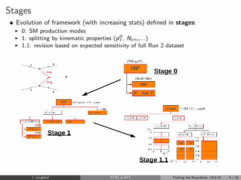
StagesEvolution of framework (with increasing stats) defined in stages:I 0: SM production modesI 1: splitting by kinematic properties (pH

T , Njets,...)I 1.1: revision based on expected sensitivity of full Run 2 dataset


Status of STXS measurements @ CMS

2016 combination of Stage 0 measurements: [Eur. Phys. J. C (2019) 79: 421]

(EW qqH)

ggF bb̄H tHtt̄HVBF

(H+ leptonic V )

V H

qq̄ →WH

qq̄ → ZH

gg → ZH

VBF

H+ had. V

(Run1-like)

ρ

1−

0.8−

0.6−

0.4−

0.2−

0

0.2

0.4

0.6

0.8

1

-0.04 0.00 0.00 0.00 0.00 -0.02 0.02 0.00 0.03 0.03 1.00

-0.67 -0.30 -0.32 -0.31 -0.20 -0.38 0.31 0.40 0.58 1.00 0.03

-0.73 -0.26 -0.07 -0.31 -0.20 -0.45 0.33 0.28 1.00 0.58 0.03

-0.27 -0.27 -0.36 -0.18 -0.13 -0.32 0.21 1.00 0.28 0.40 0.00

-0.28 -0.13 -0.09 -0.63 -0.42 -0.52 1.00 0.21 0.33 0.31 0.02

0.38 0.17 0.11 0.37 0.24 1.00 -0.52 -0.32 -0.45 -0.38 -0.02

0.18 0.08 0.06 0.24 1.00 0.24 -0.42 -0.13 -0.20 -0.20 0.00

0.28 0.12 0.09 1.00 0.24 0.37 -0.63 -0.18 -0.31 -0.31 0.00

-0.05 0.13 1.00 0.09 0.06 0.11 -0.09 -0.36 -0.07 -0.32 0.00

0.13 1.00 0.13 0.12 0.08 0.17 -0.13 -0.27 -0.26 -0.30 0.00

1.00 0.13 -0.05 0.28 0.18 0.38 -0.28 -0.27 -0.73 -0.67 -0.04

ZZ

Bgg

Hσ

ZZ

BV

BF

σ

ZZ

BH

+V

(qq)

σ

ZZ

B )ν

H+

W(l

σ

ZZ

B )ν

νH

+Z

(ll/

σ

ZZ

BttHσ

ZZ

/Bbb

B

ZZ

/BττB

ZZ

/BW

WB

ZZ

/BγγB

ZZ

/Bµ

µB

ZZ/Bµµ

B

ZZ/Bγγ

B

ZZ/BWWB

ZZ/BττB

ZZ/BbbB

ZZBttHσ

ZZB)ννH+Z(ll/σ

ZZB)νH+W(lσ

ZZBH+V(qq)σ

ZZBVBFσ

ZZBggHσ

CMSSupplementary (13 TeV)-135.9 fb

(pb

)S

MZ

Z /

BZ

Z x

Biσ 1−10

1

10

210 H→gg

VBF

H+V(qq)

)νH+W(l

)ννH+Z(ll/

ttH+tH

Stage 0 Simplified Template Cross Sections| < 2.5

H|y

Observed syst)⊕ (stat σ1± syst)⊕ (stat σ2±

(syst)σ1±SM prediction

ZZ

/ B

iB

2−10

1−10

1

10

210 bbWW

ττ

γγµµ

(13 TeV)-135.9 fbCMS


http://cms-results.web.cern.ch/cms-results/public-results/publications/HIG-17-031/index.html

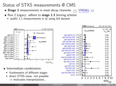
Status of STXS measurements @ CMSStage 1 measurements in most decay channels: γγ, VH(bb), ττ

Run 2 Legacy: adhere to stage 1.1 binning schemeI public 1.1 measurements in 4` using full dataset

theoσ/procσ2− 0 2 4 6 8 -0.0

+1.7 0.0 qqH other -0.0

+0.7 0.0 qqH 3J-like -0.5

+0.6 1.3 qqH 2J-like -0.0

+0.5 0.0 ggH VBF-like -1.2

+1.1 2.8 ggH 2J BSM -0.6

+0.8 0.6 ggH 2J high -1.1

+1.0 2.7 ggH 2J med -0.3

+1.4 0.3 ggH 2J low -1.5

+1.6 1.8 ggH 1J BSM -0.7

+1.0 2.0 ggH 1J high -0.4

+0.5 0.5 ggH 1J med -0.6

+0.7 1.5 ggH 1J low-0.20+0.20 1.17 ggH 0J

profiledHm

Observation

SM Prediction

Preliminary CMS

γγ→H

TeV) (13-1 77.4 fb

Intermediate combination:I frankenstein of different stagesI direct STXS meas. not possible⇒ motivates interpretations...

SMσ/σ0 1 2 3 4 5 6 7 8 9 10

-0.07+0.90 0.07H,tHtt-0.57+1.20 0.57qqH-2j/mJJ[60-120]-0.00+1.57 0.00VH/pTV>150-1.85+2.49 3.21VH/pTV[0-150]-0.00+0.73 0.00qqH-2j/pT>200-0.00+2.43 0.00qqH-rest-2.89+2.88 2.89qqH-3j/mJJ>350-0.90+1.17 0.93qqH-2j/mJJ>700-1.71+1.91 1.71qqH-2j/mJJ[350,700]-0.47+0.51 0.47ggH/pT>200-0.00+3.28 0.00ggH-2j/mJJ>350-0.75+0.87 1.16ggH-2j/pT[120-200]-0.80+0.83 1.59ggH-2j/pT[60-120]-1.13+1.35 1.47ggH-2j/pT[0-60]-0.96+1.09 1.52ggH-1j/pT[120-200]-0.51+0.41 0.82ggH-1j/pT[60-120]-0.51+0.48 0.78ggH-1j/pT[0-60]-0.17+0.18 1.06ggH-0j/pT[10-200]-0.25+0.28 0.87ggH-0j/pT[0,10]

0.06

(fb)SMσ4l→ZZ→H

0.050.030.110.020.250.040.070.050.070.100.110.230.160.100.570.882.530.80

profiledHm

(13 TeV)-1137.1 fbCMS Preliminary


http://cms-results.web.cern.ch/cms-results/public-results/preliminary-results/HIG-18-029/index.html




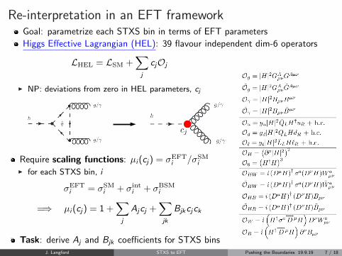
Re-interpretation in an EFT frameworkGoal: parametrize each STXS bin in terms of EFT parameters

Higgs Effective Lagrangian (HEL): 39 flavour independent dim-6 operators

LHEL = LSM +∑j

cjOj

I NP: deviations from zero in HEL parameters, cj

Require scaling functions: µi (cj) = σEFTi /σSM

iI for each STXS bin, i

σEFTi = σSM

i + σinti + σBSM

i

=⇒ µi (cj) = 1 +∑j

Ajcj +∑jk

Bjkcjck

Task: derive Aj and Bjk coefficients for STXS binsJ. Langford STXS to EFT Pushing the Boundaries 19.9.19 7 / 18

https://arxiv.org/pdf/1303.3876.pdf

EFT parametrization: derivation

µi (cj) = 1 +∑j

Ajcj +∑jk

Bjkcjck

Scaling functions for stage 1 bins calc. previously: [LHCHXSWG-INT-2017-001]I use same approach to derive Aj/Bjk for stage 0, 1 & 1.1 binsI useful for validation: compare stage 1 coefficientsI also provide decay channel parametrization: Γf (cj)

1 Generate events per Higgs prod. mode (LO): Madgraph w/ Pythia showering

2 Import HEL (UFO): reweight events for different points in HEL param space⇒ SM: all cj = 0⇒ vary cj individually: (cj = w,0,...,0), (0,w,0,...,0), ...⇒ pairwise to calc. Bjk cross terms (j 6= k): (w,w,0,...0), (w,0,w,0,...,0), ...

3 Propagate events through Rivet tool: STXS classification (0, 1 and 1.1)

4 Extract dependence of STXS bin, i , on cj (or cjck): Aj & Bjk

⇒ comparing reweighted cross section to SM

WH Leptonic


https://cds.cern.ch/record/2290628

https://gitlab.cern.ch/LHCHIGGSXS/LHCHXSWG2/STXS/Classification

EFT parametrization: stage 0

Varying cj individually...

H→gg Hqq→qq νHl→qq Hll→qq ttH→gg/qq

1−10

1

10

(a

.u.)

iσ

STXS Stage 0 HEL UFO

SM = 5e-05Gc

= 0.05HWc = 0.05Bc

= 0.01WWc = 0.5uc

OG = |H|2GAµνG

A,µνOHW = i(DµH)†σa(DνH)W a

µν OB = i(H†←→D H)∂νBµν

OWW = i(H†σa←→D H)DνW aµν Ou = yu |H2|Q̄LH

†uR + h.c.


EFT parametrization: stage 1.1 qqH

Beyond stage 0: account for shape effects as well as total rates

>25 GeV

HjjT

<200 GeV, p

HT

>700 GeV, pjj

2J, m≥

<25 GeV

HjjT

<200 GeV, p

HT

>700 GeV, pjj

2J, m≥

>25 GeV

HjjT

<200 GeV, p

HT

[350,700] GeV, p

∈jj

2J, m≥

<25 GeV

HjjT

<200 GeV, p

HT

[350,700] GeV, p

∈jj

2J, m≥

>200 GeV

HT

>350 GeV, pjj

2J, m≥

[120,350] GeV

∈jj

2J, m≥

[60,120] GeV

∈jj

2J, m≥

[0,60] GeV

∈jj

2J, m≥ 1J 0J

1−10

1

(a

.u.)

iσ

Hqq→STXS Stage 1.1 qq HEL UFO

SM = 0.05HWc = 0.2HBc = 0.03WWc

= 0.1Bc


Total scaling functionsTotal scaling: product of STXS and decay parametrizationFor signal (i ,f ):

µfi (cj) = σEFT

i /σSMi × BREFT(H→ f)/BRSM(H→ f)

I production: calculated Aj/Bjk ourselvesI decay: taken directly from [LHCHXSWG-INT-2017-001]

e.g. Stage 0

×H → γγ

10− 5− 0 5 10 15 20

)5 (10Gc

20−

15−

10−

5−

0

5

10)4 (

10Ac

2

4

6

8

10

12

) j(cf iµ

γγ → H, H →gg


Constraining the EFT parameters: χ2

Construct χ2 function: using 2016 combination stage 0 measurements

χ2 = (x − µ)TV −1(x − µ)

I x : vector of STXS measurements (cross-sections + ratios of BRs)I µ: vector of respective EFT parametrizations (functions of cj)I Vij = ρijσiσj : covariance matrix of STXS measurements (symmetrized errors)

Constraints: vary cj and extract χ2

(pb

)S

MZ

Z /

BZ

Z x

Biσ 1−10

1

10

210 H→gg

VBF

H+V(qq)

)νH+W(l

)ννH+Z(ll/

ttH+tH

Stage 0 Simplified Template Cross Sections| < 2.5

H|y

Observed syst)⊕ (stat σ1± syst)⊕ (stat σ2±

(syst)σ1±SM prediction

ZZ

/ B

iB

2−10

1−10

1

10

210 bbWW

ττ

γγµµ

(13 TeV)-135.9 fbCMS

ρ

1−

0.8−

0.6−

0.4−

0.2−

0

0.2

0.4

0.6

0.8

1

-0.04 0.00 0.00 0.00 0.00 -0.02 0.02 0.00 0.03 0.03 1.00

-0.67 -0.30 -0.32 -0.31 -0.20 -0.38 0.31 0.40 0.58 1.00 0.03

-0.73 -0.26 -0.07 -0.31 -0.20 -0.45 0.33 0.28 1.00 0.58 0.03

-0.27 -0.27 -0.36 -0.18 -0.13 -0.32 0.21 1.00 0.28 0.40 0.00

-0.28 -0.13 -0.09 -0.63 -0.42 -0.52 1.00 0.21 0.33 0.31 0.02

0.38 0.17 0.11 0.37 0.24 1.00 -0.52 -0.32 -0.45 -0.38 -0.02

0.18 0.08 0.06 0.24 1.00 0.24 -0.42 -0.13 -0.20 -0.20 0.00

0.28 0.12 0.09 1.00 0.24 0.37 -0.63 -0.18 -0.31 -0.31 0.00

-0.05 0.13 1.00 0.09 0.06 0.11 -0.09 -0.36 -0.07 -0.32 0.00

0.13 1.00 0.13 0.12 0.08 0.17 -0.13 -0.27 -0.26 -0.30 0.00

1.00 0.13 -0.05 0.28 0.18 0.38 -0.28 -0.27 -0.73 -0.67 -0.04

ZZ

Bgg

Hσ

ZZ

BV

BF

σ

ZZ

BH

+V

(qq)

σ

ZZ

B )ν

H+

W(l

σ

ZZ

B )ν

νH

+Z

(ll/

σ

ZZ

BttHσ

ZZ

/Bbb

B

ZZ

/BττB

ZZ

/BW

WB

ZZ

/BγγB

ZZ

/Bµ

µB

ZZ/Bµµ

B

ZZ/Bγγ

B

ZZ/BWWB

ZZ/BττB

ZZ/BbbB

ZZBttHσ

ZZB)ννH+Z(ll/σ

ZZB)νH+W(lσ

ZZBH+V(qq)σ

ZZBVBFσ

ZZBggHσ

CMSSupplementary (13 TeV)-135.9 fb


http://cms-results.web.cern.ch/cms-results/public-results/publications/HIG-17-031/index.html

Stage 0 combination: χ2 resultsConsider variations in subset of HEL params:⇒ cG , cA, cu, cd , cl , cHW , cWW − cBI leading terms in measured processes + not tightly constrained by other dataI not including CP-odd operators: do not enter STXS observables at leading-orderI S = cWW + cB : precision EWK param, strong exp. constraintI fix other cj = 0

Solid: profile other HEL params. Dashed: fix other HEL params to 0

10 5 0 5 10

cG x 105

0

2

4

6

8

10

∆χ

2

Profile cj

Fix cj = 0

6

5

4

3

2

1

0

1

2

3

Pro

file

d E

FT c

oeff

.

cu_x01

cl

cd_x01

cA_x04

cWWMinuscB_x02

cHW_x02

10 5 0 5 10

cA x 104

0

2

4

6

8

10

∆χ

2

Profile cj

Fix cj = 0

15

10

5

0

5

10

Pro

file

d E

FT c

oeff

.

cu_x01

cl

cG_x05

cd_x01

cWWMinuscB_x02

cHW_x02

cG constraint primarily from ggH, cA from H→ γγ


Stage 0 combination: χ2 results


15 10 5 0 5 10 15 20

cHW x 102

0

2

4

6

8

10

∆χ

2

Profile cj

Fix cj = 0

8

6

4

2

0

2

4

6

8

10

Pro

file

d E

FT c

oeff

.

cu_x01

cl

cA_x04

cd_x01

cWWMinuscB_x02

cG_x05

15 10 5 0 5 10 15

(cWW − cB) x 102

0

2

4

6

8

10

∆χ

2

Profile cj

Fix cj = 0

10

5

0

5

10

Pro

file

d E

FT c

oeff

.

cu_x01

cl

cHW_x02

cA_x04

cd_x01

cG_x05

Both affect HVV vertices ⇒ constraints from VBF + VH


Stage 0 combination: χ2 results


Ou: affects Htt vertex ⇒ constraint from ttH

20 15 10 5 0 5 10

cu x 101

0

1

2

3

4

5

µ

ggH_hzz_

qqH_hzz_

ttH_hzz_

ZH_lep_hzz_

WH_lep_hzz_

R_BR_hbbBR_hzz_

R_BR_httBR_hzz_

VH_had_hzz_

R_BR_hwwBR_hzz_

R_BR_hggBR_hzz_

20 15 10 5 0 5 10

cu x 101

0

2

4

6

8

10

∆χ

2

Profile cj

Fix cj = 0

10

5

0

5

10

Pro

file

d E

FT c

oeff

.

cl

cG_x05

cA_x04

cd_x01

cWWMinuscB_x02

cHW_x02

Turning point in µ for ttH: two values of cu give µ = 1

Leads to double minimum in χ2 distribution

Rest of χ2 distributions + scaling functions in Back-up


Stage 0 combination: summary

20− 15− 10− 5− 0 5 10Parameter value

x 10uc

x 10lc

5 x 10G

c

4 x 10A

c

x 10d

c

2) x 10B

c− WW

(c

2 x 10HW

c

(13 TeV)-135.9 fb

Observed

σ1±

σ2±


CMS Higgs Combination: EFT interpretation

Run 2 Legacy: stage 1.1 combination of major H decay channelsI direct XS measurements + interpretation

Intermediate combinations: mixture of stage 0, 1 and 1.1 processesI binning schemes not backwards compatible: direct XS measurements not possibleI EFT interpretation is: now have complete set of µf

i (HEL)

For final results: χ2 ⇒ full maximum-likelihood fitI confine signal process (i ,f ) to scale according to relevant µf

i (cj)I likelihood scan over cj ⇒ extract constraints

Transition from HEL to SMEFT interpretation (SMEFTsim model)I change of basis (SILH → Warsaw)I permits combinations with other areas of HEP: VBS, top, SM


https://arxiv.org/pdf/1709.06492.pdf

Summary

Summarised status of STXS measurements in CMS

EFT interpretation of STXSI derived µi (cj): describe how XS scales as function of HEL parameters

Presented results based on χ2 analysis of CMS 2016 Higgs combination


Back-Up Slides


χ2 results: cG

10 5 0 5 10

cG x 105

0.0

0.5

1.0

1.5

2.0

2.5

µ

ggH_hzz_

qqH_hzz_

ttH_hzz_

ZH_lep_hzz_

WH_lep_hzz_

R_BR_hbbBR_hzz_

R_BR_httBR_hzz_

VH_had_hzz_

R_BR_hwwBR_hzz_

R_BR_hggBR_hzz_

10 5 0 5 10

cG x 105

0

2

4

6

8

10

∆χ

2

Profile cj

Fix cj = 0

6

5

4

3

2

1

0

1

2

3

Pro

file

d E

FT c

oeff

.

cu_x01

cl

cd_x01

cA_x04

cWWMinuscB_x02

cHW_x02


χ2 results: cA

10 5 0 5 10

cA x 104

0.0

0.5

1.0

1.5

2.0

2.5

µ

ggH_hzz_

qqH_hzz_

ttH_hzz_

ZH_lep_hzz_

WH_lep_hzz_

R_BR_hbbBR_hzz_

R_BR_httBR_hzz_

VH_had_hzz_

R_BR_hwwBR_hzz_

R_BR_hggBR_hzz_

10 5 0 5 10

cA x 104

0

2

4

6

8

10

∆χ

2

Profile cj

Fix cj = 0

15

10

5

0

5

10

Pro

file

d E

FT c

oeff

.

cu_x01

cl

cG_x05

cd_x01

cWWMinuscB_x02

cHW_x02


χ2 results: cHW

15 10 5 0 5 10 15 20

cHW x 102

0

5

10

15

20

25

30

µ

ggH_hzz_

qqH_hzz_

ttH_hzz_

ZH_lep_hzz_

WH_lep_hzz_

R_BR_hbbBR_hzz_

R_BR_httBR_hzz_

VH_had_hzz_

R_BR_hwwBR_hzz_

R_BR_hggBR_hzz_

15 10 5 0 5 10 15 20

cHW x 102

0

2

4

6

8

10

∆χ

2

Profile cj

Fix cj = 0

8

6

4

2

0

2

4

6

8

10

Pro

file

d E

FT c

oeff

.

cu_x01

cl

cA_x04

cd_x01

cWWMinuscB_x02

cG_x05


χ2 results: cWW − cB

15 10 5 0 5 10 15

(cWW − cB) x 102

0

2

4

6

8

10

12

14

16

µ

ggH_hzz_

qqH_hzz_

ttH_hzz_

ZH_lep_hzz_

WH_lep_hzz_

R_BR_hbbBR_hzz_

R_BR_httBR_hzz_

VH_had_hzz_

R_BR_hwwBR_hzz_

R_BR_hggBR_hzz_

15 10 5 0 5 10 15

(cWW − cB) x 102

0

2

4

6

8

10

∆χ

2

Profile cj

Fix cj = 0

10

5

0

5

10

Pro

file

d E

FT c

oeff

.

cu_x01

cl

cHW_x02

cA_x04

cd_x01

cG_x05


χ2 results: cu

20 15 10 5 0 5 10

cu x 101

0

1

2

3

4

5

µ

ggH_hzz_

qqH_hzz_

ttH_hzz_

ZH_lep_hzz_

WH_lep_hzz_

R_BR_hbbBR_hzz_

R_BR_httBR_hzz_

VH_had_hzz_

R_BR_hwwBR_hzz_

R_BR_hggBR_hzz_

20 15 10 5 0 5 10

cu x 101

0

2

4

6

8

10

∆χ

2

Profile cj

Fix cj = 0

10

5

0

5

10

Pro

file

d E

FT c

oeff

.

cl

cG_x05

cA_x04

cd_x01

cWWMinuscB_x02

cHW_x02


χ2 results: cd

20 15 10 5 0 5 10

cd x 101

0

1

2

3

4

5

6

7

µ

ggH_hzz_

qqH_hzz_

ttH_hzz_

ZH_lep_hzz_

WH_lep_hzz_

R_BR_hbbBR_hzz_

R_BR_httBR_hzz_

VH_had_hzz_

R_BR_hwwBR_hzz_

R_BR_hggBR_hzz_

20 15 10 5 0 5 10

cd x 101

0

2

4

6

8

10

∆χ

2

Profile cj

Fix cj = 0

15

10

5

0

5

10

15

Pro

file

d E

FT c

oeff

.

cu_x01

cl

cG_x05

cA_x04

cWWMinuscB_x02

cHW_x02


χ2 results: c`

2.0 1.5 1.0 0.5 0.0 0.5 1.0 1.5 2.0

cl

0

2

4

6

8

10

12

14

16

µ

ggH_hzz_

qqH_hzz_

ttH_hzz_

ZH_lep_hzz_

WH_lep_hzz_

R_BR_hbbBR_hzz_

R_BR_httBR_hzz_

VH_had_hzz_

R_BR_hwwBR_hzz_

R_BR_hggBR_hzz_

2.0 1.5 1.0 0.5 0.0 0.5 1.0 1.5 2.0

cl

0

2

4

6

8

10

∆χ

2

Profile cj

Fix cj = 0

10

5

0

5

10

15

Pro

file

d E

FT c

oeff

.

cu_x01

cG_x05

cA_x04

cd_x01

cWWMinuscB_x02

cHW_x02


an eft interpretation of stxs measurements at cms

Documents