an efficient stream-based join to process end user ...dline.info/fpaper/jdim/v12i3/5.pdf ·...

Journal of Digital Information Management Volume 12 Number 3 June 2014 201

An Efficient Stream-based Join to Process End User Transactions in Real-Time Data Warehousing

M. Asif Naeem1, Noreen Jamil21School of Computing and Mathematical SciencesAuckland University of TechnologyAuckland, New Zealand

2Department of Computer ScienceThe University of AucklandAuckland, New [email protected], [email protected]

Journal of DigitalInformation Management

ABSTRACT: In the field of real-time data warehousingsemistream processing has become a potential area ofresearch since last one decade. One important operationin semi-stream processing is to join stream data with aslowly changing diskbased master data. A join operatoris usually required to implement this operation. This joinoperator typically works under limited main memory andthis memory is generally not large enough to hold thewhole disk-based master data. Recently, a seminal joinalgorithm called MESHJOIN (Mesh Join) has beenproposed in the literature to process semistream data.MESHJOIN is a candidate for a resource-aware systemsetup. However, MESHJOIN is not very selective. Inparticular, MESHJOIN does not consider thecharacteristics of stream data and its performance issuboptimal for skewed stream data. In this paper wepropose a novel Semi-Stream Join (SSJ) using a newcache module. The algorithm is more appropriate forskewed distributions, and we present results for Zipfiandistributions of the type that appears in many applications.We present the cost model for our SSJ and validate itwith experiments. Based on the cost model we also tunethe algorithm up to a maximum performance. We conducta rigorous experimental study to test our algorithm. Ourexperiments show that SSJ outperforms MESHJOINsignificantly.

Subject Categories and Descriptors:

H.2.7 [Database Administration]; Data Warehouse andRepository: H.2.4 [Systems]; Transaction ProcessingI.2H.2

General Terms: Data Warehousing, Data Processing

Keywords: Real-time Data Warehousing, Semi-streamProcessing, Join Operator, Performance Measurement

Received: 3 January 2014, Revised 13 January 2014, Accepted9 February 2014

1. Introduction

In the field of Data Stream Management (DSM), streamprocessing due to its infinite characteristics has becomea potential area of research over the last decade. Datastream processing deals with continuously arrivinginformation, which is important for many differentapplications such as network traffic monitoring [1], sensordata [2], web log analysis [3], online auctions [4], andsupply-chain management [5]. One kind of streamprocessing is to join single stream data with slowlychanging disk-based data using a stream-based joinoperator. A typical example of such type of streamprocessing is in real-time data warehousing [6] [7]. In thisapplication, the slowly changing data is typically a masterdata table while incoming real-time sales data (also calledend user transactions) is a stream data. The stream basedjoin can be used for example to replace data source keywith warehouse key or enrich the stream data with masterdata. The most natural type of join in this scenario wouldbe an equijoin, performed for example on a foreign key inthe stream data.

202 Journal of Digital Information Management Volume 12 Number 3 June 2014

In the literature, a well known semi-stream algorithmMESHJOIN [8] [9] was proposed for joining a continuousstream data with a disk-based master data, such as thescenario in active data warehouses. The MESHJOINalgorithm is a hash join, where the stream serves as thebuild input and the disk-based relation serves as the probeinput.

The algorithm performs a staggered execution of the hashtable build in order to load in stream tuples more steadily.Although the MESHJOIN algorithm efficiently amortizesthe disk I/O cost over fast input streams, the algorithmmakes no assumptions about characteristics of streamdata or the organization of the master data. Experimentsby the MESHJOIN authors have shown that the algorithmperforms worse with skewed data. Therefore, the questionremains how much potential for improvement remainsuntapped due to the algorithm not being consider thecharacteristics of stream data.

In this paper we focus on one of the most commoncharacteristics, a skewed distribution. Such distributionsarise in practice, for example current economic modelsshow that in many markets a selective few products arebought with higher frequency [10]. Therefore, in the inputstream, the end user transactions related to thoseproducts are the most frequent. In MESHJOIN, thealgorithm does not consider the frequency of streamtuples.

We propose a robust algorithm called Semi-Stream Join(SSJ). The key feature of SSJ is that the algorithm storesthe most used portion of the disk-based relation, whichmatches the frequent items in the stream, in memory. Asa result, this reduces the I/O cost substantially, whichimproves the performance of the algorithm. Since ourpurpose is primarily to gauge performance with skeweddistributions, we consider a very clean, artificial as wellas real datasets that exactly exhibit a well-understoodtype of skew, a power law.

The rest of the paper is structured as follows. Section IIpresents related work. The existing MESHJOIN andproblem statement are defined in Section III. Section IVdescribes the proposed SSJ with its execution architectureand cost model. Section V-A presents the extension ofSSJ in the form of tuning. Section VI describes anexperimental study of SSJ. Finally, Section VII concludesthe paper.

2. Related Work

In this section we will outline the well known work thathas already been done in this area with a particular focuson those which are closely related to our problem domain.

The non-blocking symmetric hash join (SHJ) [11] promotesthe proprietary hash join algorithm by generating the joinoutput in a pipeline. In the symmetric hash join there is aseparate hash table for each input relation. When the tuple

of one input arrives it probes the hash table of the otherinput, generates a result and stores it in its own hashtable. SHJ can produce a result before reading either inputrelation entirely, however, the algorithm keeps both thehash tables, required for each input, in memory. EarlyHash Join (EHJ) [12] is a further extension of SHJ.

The Double Pipelined Hash Join (DPHJ) [13] with a twostage join algorithm is an extension of SHJ. The XJoinalgorithm [14] is another extension of SHJ. Hash-MergeJoin (HMJ) [15] is also one based on symmetric joinalgorithm. It is based on push technology and consists oftwo phases, hashing and merging.

Early Hash Join (EHJ) [12] is a further extension of SHJ.EHJ introduces a new biased flushing policy that flushesthe partitions of the largest input first. EHJ also simplifiesthe strategies to determine the duplicate tuples, basedon cardinality and therefore no timestamps are requiredfor arrival and departure of input tuples. However, becauseEHJ is based on pull technology, a reading policy isrequired for inputs.

R-MESHJOIN (reduced Mesh Join) [16] clarifies thedependencies among the components of MESHJOIN. Asa result, it improves the performance slightly. However, R-MESHJOIN again does not consider the non-uniformcharacteristic of stream data.

One approach to improve MESHJOIN is a partitionbasedjoin algorithm [17] that can also deal with streamintermittence. It uses a two-level hash table for attemptingto join stream tuples as soon as they arrive, and uses apartition-based waiting area for other stream tuples. Forthe algorithm in [17], however, the time that a tuple iswaiting for execution is not bounded. We are interestedin a join approach where there is a time guarantee forwhen a stream tuple will be joined.

Another recent approach, Semi-Streaming Index Join(SSIJ) [18] joins stream data with disk-based data. SSIJuses page level cache i.e. stores the entire disk pages incache while it is possible that all the tuples in these pagesmay not be frequent in stream. As a result the algorithmcan perform suboptimal. Also the algorithm does notinclude the mathematical cost model.

3. Preliminaries and Problem Definition

In this section we summarize the MESHJOIN algorithmand at the end of the section we describe the observationsthat we focus on in this paper.

MESHJOIN was designed to process stream data (alsocalled end user transactions) with disk-based master data(also called disk-based relation) in the field of real timedata warehousing. The algorithm reads the disk-basedrelation R sequentially in segments. Once the last segmentis read, it again starts from the first segment. The algorithmcontains a buffer, called the disk buffer, to store each


segment in memory one at a time, and has a number ofmemory partitions, equal in size, to store the streamtuples. These memory partitions behave like a queue andare differentiated with respect to the loading time. Thenumber of partitions is equal to the number of segmentson the disk while the size of each segment on the disk isequal to the size of the disk buffer. In each iteration thealgorithm reads one disk segment into the disk buffer andloads a chunk of stream tuples into the memory partition.After loading the disk segment into memory it joins eachtuple from that segment with all stream tuples available indifferent partitions. Before the next iteration the oldeststream tuples are expired from the join memory and allchunks of the stream are advanced by one step. In thenext iteration the algorithm replaces the current disksegment with the next one, loads a chunk of stream tuplesinto the memory partition, and repeats the above procedure.

The MESHJOIN algorithm successfully amortizes the fastarrival rate of the incoming stream by executing the joinof disk pages with a large number of stream tuples.However there are still some further issues that exist inthe algorithm. MESHJOIN does not consider thecharacteristic of skew in stream data. Experiments bythe MESHJOIN authors have shown that the algorithmperforms suboptimal with skewed data.

4. Semi-stream Join (SSJ)

In this paper, we propose a new algorithm, Semi-StreamJoin (SSJ), that overcomes the issues stated in abovesection. This section gives a detail overview of the SSJalgorithm and presents its cost model.

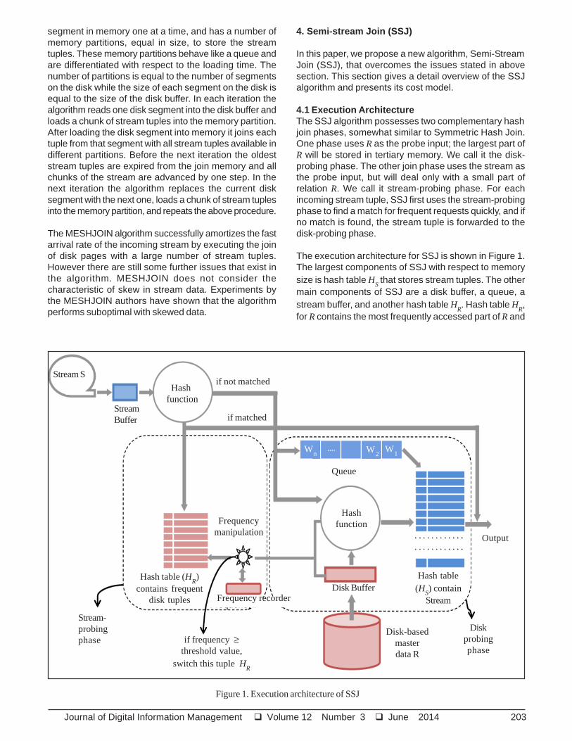
4.1 Execution ArchitectureThe SSJ algorithm possesses two complementary hashjoin phases, somewhat similar to Symmetric Hash Join.One phase uses R as the probe input; the largest part ofR will be stored in tertiary memory. We call it the disk-probing phase. The other join phase uses the stream asthe probe input, but will deal only with a small part ofrelation R. We call it stream-probing phase. For eachincoming stream tuple, SSJ first uses the stream-probingphase to find a match for frequent requests quickly, and ifno match is found, the stream tuple is forwarded to thedisk-probing phase.

The execution architecture for SSJ is shown in Figure 1.The largest components of SSJ with respect to memorysize is hash table H

S that stores stream tuples. The other

main components of SSJ are a disk buffer, a queue, astream buffer, and another hash table H

R. Hash table H

R,

for R contains the most frequently accessed part of R and

Figure 1. Execution architecture of SSJ

Stream S

Hash function

StreamBuffer

if not matched

if matched

Frequencymanipulation

Stream-probingphase if frequency ≥

threshold value,switch this tuple H

R

Hash table (HR)

contains frequentdisk tuples Frequency recorder

Disk-basedmasterdata R

Queue

Hashfunction

Disk Buffer

Diskprobingphase

Hash table(H

S) contain

Stream

Output

W1W

2W

n....


is stored permanently in memory. Relation R and streamS are the external input sources.

SSJ alternates between the stream-probing and thediskprobing phases. The hash table H

S is used to store

only that part of the update stream that does not matchtuples in H

R. A stream-probing phase ends if H

S is

completely filled or if the stream buffer is empty. Then thedisk-probing phase becomes active. In each iteration ofthe disk-probing phase, the algorithm loads a set of tuplesof R into memory to amortize the costly disk access.After loading the disk pages into the disk buffer, thealgorithm probes each tuple of the disk buffer in the hashtable H

S. If the required tuple is found in H

S, the algorithm

generates that tuple as an output. After each iteration thealgorithm removes the oldest chunk of stream tuples fromH

S. This chunk is found at the top of the queue; its tuples

were joined with the whole of R and are thus completelyprocessed now.

As the algorithm reads R sequentially, no index on R isrequired. After one iteration of disk-probing phase, asufficient number of stream tuples are deleted from H

S, so

the algorithm switches back to the stream-probing

Lines 2 to 9 specify the stream-probing phase. In thisphase the algorithm reads w stream tuples from the streambuffer (line 2). After that the algorithm probes each tuple tof w in the disk-build hash table H

R, using an inner loop

phase. One phase of stream-probing with a subsequentphase of disk-probing constitutes one outer iteration ofSSJ.

The stream-probing phase (also called cache module) isused to boost the performance of the algorithm by quicklymatching the most frequent master data. For determiningvery frequent tuples in R and loading them into H

R, the

frequency detection process is required. This processtests whether the matching frequency of the current tupleis larger than a pre-set threshold. If it is, then this tuple isentered into H

R. If there are no empty slots in H

R the

algorithm overwrites an existing least frequent tuple inH

R. This least frequent tuple is determined by the

component frequency recorder.

An important question is how frequently a master datatuple must be used in order to get into this phase, so thatthe memory sacrificed for this phase really delivers aperformance advantage. In Section V-A we give a precise

Algorithm 1 SSJ

Input: A disk based relation R and a stream of updates S

Output: R S

Parameters: w (where w = wS + wN) tuples of S and b tuplesof R.

Method:

1: while (true) do2: READ w stream tuples from the stream buffer3: for each tuple t in w do4: if t ∈ H

R then

5: OUTPUT t6: else7: ADD stream tuple t into H

S and also place its

pointer value into Q8: end if9: end for10: READ b number of tuples of R into the disk buffer11: for each tuple r in b do12: if r ∈ H

S then

13: OUTPUT r14: f ← number of matching tuples found in H

S15: if (f ≥ thresholdValue) then16: SWITCH the tuple r into hash table H

R17: end if18: end if19: end for20: DELETE the oldest w tuples from H

S along with

their corresponding pointers from Q21: end while


and comprehensive analysis that shows that a remarkablysmall amount of memory assigned to the stream-probingphase can deliver a substantial performance gain.

4.2 AlgorithmThe execution steps for SSJ are shown in Algorithm 1.The outer loop of the algorithm is an endless loop, whichis common in stream processing algorithms (line 1). Thebody of the outer loop has two main parts: the stream-probing phase and the disk-probing phase. Due to theendless loop, these two phases alternate.

Lines 2 to 9 specify the stream-probing phase. In thisphase the algorithm reads w stream tuples from the streambuffer (line 2). After that the algorithm probes each tuple tof w in the disk-build hash table H

R, using an inner loop

(line 3). In the case of a match, the algorithm generatesthe join output without storing t in H

S. In the case where t

does not match, the algorithm loads t into HS, while also

enqueuing its pointer in the queue Q (lines 4-8).

Lines 10 to 20 specify the disk-probing phase. At the startof this phase, the algorithm reads b tuples from R andloads them into the disk buffer (line 10). In an inner loop,the algorithm looks up all tuples from the disk buffer inhash table H

S. In the case of a match, the algorithm

generates that tuple as an output (lines 11 to 13). Since

HS is a multihash-map, there can be more than one match;

the number of matches is f (line 14).

Lines 15 and 16 are concerned with frequency detection.In line 15 the algorithm tests whether the matchingfrequency f of the current tuple is larger than a pre-setthreshold. If it is, then this tuple is entered into H

R. If there

are no empty slots in HR, the algorithm overwrites an

existing least-frequent tuple in HR using the frequency

recorder. Finally, the algorithm removes the expired streamtuples (i.e. the ones that have been joined with the wholeof R) from H

S, along with their pointer values from the queue

(line 20). If the cache is not full, this means the thresholdis too high; in this case, the threshold can be loweredautomatically. Similarly, the threshold can be raised iftuples are evicted from the cache too frequently. Thismakes the stream-probing phase flexible and able to adaptonline to changes in the stream behavior. Necessarily, itwill take some time to adapt to changes, similar to thewarmup phase. However, this is usually deemedacceptable for a stream-based join that is supposed torun for a long time.

4.3 Cost modelIn this section we develop the cost model for our proposedSSJ. The main objective for developing our cost model is

Parameter name Symbol

Total allocated memory (bytes) M

Service rate (processed tuples/sec) µNumber of stream tuples processed in each iteration through H

R w

N

Number of stream tuples processed in each iteration through HS

wS

Disk page size (bytes) vP

Disk buffer size (pages) k

Disk buffer size (tuples) d

Size of HR (pages) l

Size of HR (tuples) h

R

Size of HS (tuples) h

S

Disk relation size (tuples) Rt

Memory weight for the hash table

Memory weight for the queue 1−αCost to look-up one tuple in the hash table (nano secs) c

H

Cost to generate the output for one tuple (nano secs) cO

Cost to remove one tuple from the hash table and the queue (nano secs) cE

Cost to read one stream tuple into the stream buffer (nano secs) cS

Cost to append one tuple in the hash table and the queue (nano secs) cA

Cost to compare the frequency of one disk tuple with the specified threshold value (nano secs) cF

Total cost for one loop iteration (secs) cloop

Table 1. Notations used in cost estimation of SSJ


to interrelate the key parameters of the algorithm, suchas input size w, processing cost c

loop for these w tuples,

the available memory M and the service rate µ. The costmodel presented here follows the style used for MESHJOIN[9] [8]. Equation 1 represents the total memory used bythe algorithm (except the stream buffer), and Equation 2describes the processing cost for each iteration of thealgorithm. The notations we used in our cost model aregiven in Table 1.

4.3.1 Memory costThe major portion of the total memory is assigned to thehash table H

S together with the queue while a

comparatively much smaller portion is assigned to HR and

the disk buffer. The memory for each component can becalculated as follows:

Memory for disk buffer (bytes) = k.vP

Memory for HR (bytes) = l.vP

Memory for frequency recorder (bytes) = 8hR

Memory for HS (bytes) = [M − (k + l) vP 8hR]

Memory for the queue (bytes) = (1 − α) [M − (k + l) vP 8hR]

By aggregating the above, the total memory for SSJ canbe calculated as shown in Equation 1.

M = (k + l) vP + 8hR + α [M − (k + l) vP − 8hR]

+ (1− α) [M (k + l) vP − 8hR]

Currently, the memory for the stream buffer in not includedbecause it is small (0.05 MB is sufficient in ourexperiments).

4.3.2 Processing costIn this section we calculate the processing cost for thealgorithm. To make it simple we first calculate theprocessing cost for individual components and then sumthese costs to calculate the total processing cost for oneiteration.

cI/O

(k .vP) = Cost to read k pages into the disk buffer

wN.cH = Cost to look-up wN tuples in HR

d.cH = Cost to look-up disk buffer tuples in HS

d.cF = Cost to compare the frequency of all the tuples in

disk buffer with the threshold value

wN.c

O = Cost to generate the output for w

N tuples

wS.cO = Cost to generate the output for wS tuples

wN.cS = Cost to read the wN tuples from the stream buffer

wS.c

S = Cost to read the w

S tuples from the stream buffer

wS.c

A = Cost to append w

S tuples into H

S and the queue

wS.cE = Cost to delete wS tuples from HS and the queue

By aggregating the above costs the total cost of thealgorithm for one iteration can be calculated using

Equation 2.

cloop

(secs) = 10− 9 [cI/O

(k.vP) + d (c

H + c

F) + w

s

(cO+ c

E + c

S + c

A) + w

N (c

H + c

O + c

S)]

The term 10− 9 is a unit conversion from nanoseconds toseconds. In c

loop seconds the algorithm processes w

N

and wS tuples of the stream S, the service rate µ can be

calculated using Equation 3.

wN + wS

cloopµ =

5. Extensions

This section presents the tuning of SSJ as an ourextended work.

5.1 TuningAs we have outlined in the abstract, we assume that onlylimited resources are available for SSJ. Hence we face atrade-off with respect to memory distribution. Assigningmore memory to one component means assigning equallyless memory to some other components. Therefore, toutilize the available memory optimally, tuning of the joincomponents is important. If the size of R and the overallmemory size M is fixed, the equation is a function of twoparameters, the size for disk buffer and the size of hashtable H

R.

The tuning of the algorithm uses the cost model that wehave derived. Therefore we decided to use the tuning ofthe algorithm to experimentally validate the cost model.We not only provide a theoretical approach to tuning, basedon calculus of variations. We first approximate optimaltuning settings using an empirical approach, byconsidering a sample of values for the disk buffer andhash table H

R. Finally we compare the experimentally

obtained tuning results with the results obtained basedon the cost model.

5.1.1 Empirical TuningThis section focuses on obtaining samples for theapproximate tuning of the key components. Since, theperformance is a function of two variables, the size of thedisk buffer, d, and the size of hash table H

R, h

R. We tested

the performance of the algorithm for a grid of values forboth components, i.e. for each setting of d the performanceis measured against a series of values for h

R. The

performance measurements for the grid of d and hR are

shown in Figure 2. It is worth following the data along theh

R axis, i.e. for a fixed d we look at all values for h

R. This

will show that a stream-probing phase is useful if it remainswithin a certain size. This is so, because in the beginningthe performance increases rapidly with an increase in h

R.

Then, after reaching an optimum the performancedecreases. The explanation is that when h

R is increased

beyond this value, it does not make any significant

(1)

(2)

(3)


Figure 2. Tuning of SSJ using measurement approach

difference to the stream matching probability due to thecharacteristics of the skewed distribution. On the otherhand it reduces the memory for hash table H

S. Similarly

we can follow the data along the d axis. Initially theperformance increases, since the costly disk access isamortized for a larger number of stream tuples. This effectis actually of crucial importance, because it is this gainthat gives the algorithm an advantage over a simple index-based join. It is here that H

S is used in order to match

more tuples than just the one that was used in order todetermine the partition that was loaded. After attaining amaximum, the performance decreases because of theincrease in I/O cost for loading more of R at one time in anon-selective way.

From the figure the optimal memory settings for both diskbuffer and hash table H

R can be determined by considering

the intersection of the values of both components at whichthe algorithm individually performs at a maximum.

5.1.2 Tuning based on cost modelWe now show how the cost model for SSJ can be used to(theoretically) obtain an optimal tuning of the components.Equation 1 and 2 represents the memory and processingcost respectively for the algorithm. On the basis of theseequations the performance of the algorithm can becalculated using Equation 3.

The algorithm can be tuned to perform optimally usingEquation 3 by knowing w

N, w

N and c

loop. The value of cloop

can be calculated from Equation 2 if we know wN and w

S.

Mathematical model for wN: SSJ has two separatephases, the stream-probing and the disk-probing phase.The stream tuples that are matched in the stream-probingphase are joined straight away without storing them inH

S. The number of tuples processed through this phase

per outer iteration are denoted by wN.

The main components that directly affect wN are the sizeof the master data on disk and the size of H

R. To calculate

the effect of both components on wN we assume that Rt

is the total number of tuples in R while hR is the size of H

Rin terms of tuples. We now use our assumption that thestream of updates S has a Zipfian distribution withexponent value one. In this case the matching probabilityfor S in the stream-probing phase can be determined usingEquation 4. The denominator is a normalization term toensure all probabilities sum up to 1.

pN =

Σ

Σ

h

x = 1

x = 1

R

Rt 1x

1x

11500

11000

10500

10000

9500

9000

8500

8000

7500

7000

9001000

800

700

500

600

10001500

2000

25003000

3500

Size f disk buffer. h R (tuples)

Size f disk buffer. d (tuples)

Serv

ice

rate

(tup

les/

sec)

(4)


Each summation in the above equation generates theharmonic series which can be summed up using formula

= ln k + γ + εk [19], where γ is Euler’s constantΣ

x = 1

k 1x

whose value is approximately equal to 0.5772156649 and

εk is another constant which is ≈ 12k

. The value of εk appro-

aches 0 as k goes to ∞ [19]. In our case the value of12k

is small so we ignore it. Hence Equation 4 can be writtenas shown in Equation 5.

pN =In h

R

In Rt

Now using Equation 5 we can determine the constantfactors of change in pN by changing the values of hR andRt individually. Let us assume that pN decreases withconstant factor φN by doubling the value of Rt and increasewith constant factor ψN by doubling the value of hR.Knowing these constant factors we are able to calculatethe value of wN. Let us assume the following:

pN

= Rt h

R

y z

Dividing the above equation by Equation 6 we get 2y = φ

N

and therefore, y = log2 (φ

N):

Determination of z: Similarly we also know that by doublingh

R the matching probability p

N increases by a constant

factor N therefore, Equation 6 can be written as:

ψNpN = (2Rt )yhR )

2z

By dividing the above equation by Equation 6 we get 2z =ψN and therefore, 2z = log

2 (ψN). After substituting the values

of constants y and z into Equation 6 we get:

pN

= Rtlog (φ

)

2 N hR

log (ψ

)2 N

Now if Sn is the total number of stream tuples that areprocessed (through both phases) in n outer iterations thenwN can be calculated using Equation 7.

wN

=

log (φ

)2 N h

R

log (ψ

)2 N(R

t )Sn

n

Mathematical model for wS : The second phase of theSSJ algorithm deals with the rest of R. This part is calledR′, with R′ = R − h

R. The algorithm reads R′ in segments.

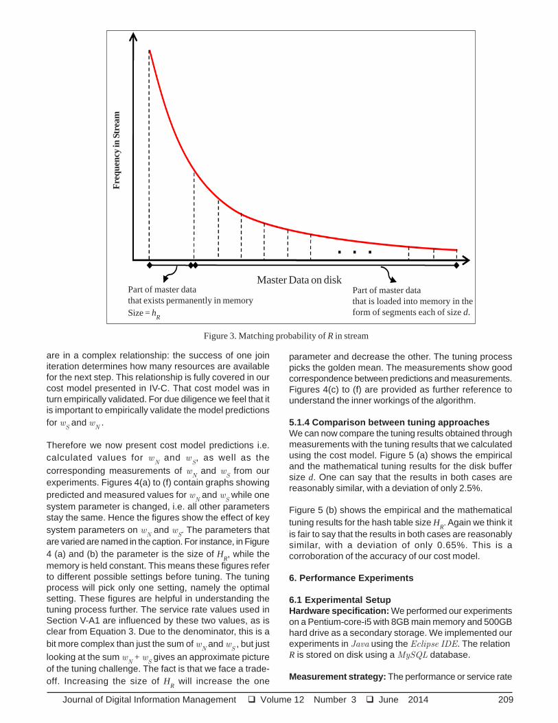
The size of each segment is equal to the size of the diskbuffer d. In each iteration the algorithm reads one segmentof R′ using an index on the join attribute and loads it intothe disk buffer. Since we assume a skewed distribution,the matching probability is not equal, but decreases inthe tail of the distribution, as shown in Figure 3. Wecalculate the matching probability for each segment bysumming over the discrete Zipfian distribution separatelyand then aggregating all of them as shown below.

Σh

x =

+R

1x

+ d

hR + 1Σ

h

x =

+R

1x

+ 2d

hR+ d +1Σ

h

x =

+...+R

1x

+ 3d

hR+ 2d +1

Σh

x =

R 1x

+ nd

hR + (n − 1)d +1

We simplify this to:

Σh

x =

R1x

+ nd

hR + 1

⇒ ΣR

x =

t

hR + 1

1x

From this we can obtain the average matching probabilityp

S in the disk-probing phase, which we need for calculating

wS. Let N be the total number of segments in R′. In the

denominator, we have to use the same normalization termas in Equation 4.

ΣR

x =

t

hR + 1

1x

ΣR

x = 1

t1xN

pS =

We again use the summation formula [19]:

In (Rt) − In (hR)

N (In (Rt) + γ )pS =

To determine the effects of d, hR and Rt on pS, a similarargument can be used as in the case of wN . Let’s supposewe double d in Equation 8, then N will be halved and thevalue of pS increases by a constant factor of S. Similarly,if we double hR or Rt respectively, then the value of pS

decreases by some constant factor of ψS or φS respectively.Using a similar argument for wN, we get:

pS = dx hR Rt

y z

The values for the constants x, y and z in this case will bex = log

2(θ

S), y = log

2(ψ

S) and z = log

2(φ

S) respectively.

Therefore by replacing the values with constants Equation9 will become.

pS = dlog (θ

)

2 S hR

log (ψ

)2 S R

t

log (φ

)2 S

Now if hS are the number of stream tuples stored in the

hash table then the average value for wS can be calculated

using Equation 10.

wS

(average) = dlog (θ

)

2 S hR

log (ψ

)2 S Rt

log (φ

)2 S hS

Once the values of wN and wS are determined, the algorithmcan be tuned using Equation 3.

5.1.3 Comparison of cost model and measurementsThe terms wS and wN are of crucial importance in ourunderstanding of SSJ. This is so, firstly because theyrefer to the functioning of both join phases. Secondly they

(5)

(6)

(7)

(8)

(9)

(10)


Figure 3. Matching probability of R in stream

are in a complex relationship: the success of one joiniteration determines how many resources are availablefor the next step. This relationship is fully covered in ourcost model presented in IV-C. That cost model was inturn empirically validated. For due diligence we feel that itis important to empirically validate the model predictionsfor w

S and w

N .

Therefore we now present cost model predictions i.e.calculated values for w

N and w

S, as well as the

corresponding measurements of wN and w

S from our

experiments. Figures 4(a) to (f) contain graphs showingpredicted and measured values for w

N and w

S while one

system parameter is changed, i.e. all other parametersstay the same. Hence the figures show the effect of keysystem parameters on w

N and w

S. The parameters that

are varied are named in the caption. For instance, in Figure4 (a) and (b) the parameter is the size of H

R, while the

memory is held constant. This means these figures referto different possible settings before tuning. The tuningprocess will pick only one setting, namely the optimalsetting. These figures are helpful in understanding thetuning process further. The service rate values used inSection V-A1 are influenced by these two values, as isclear from Equation 3. Due to the denominator, this is abit more complex than just the sum of w

N and w

S , but just

looking at the sum wN + w

S gives an approximate picture

of the tuning challenge. The fact is that we face a trade-off. Increasing the size of H

R will increase the one

parameter and decrease the other. The tuning processpicks the golden mean. The measurements show goodcorrespondence between predictions and measurements.Figures 4(c) to (f) are provided as further reference tounderstand the inner workings of the algorithm.

5.1.4 Comparison between tuning approachesWe can now compare the tuning results obtained throughmeasurements with the tuning results that we calculatedusing the cost model. Figure 5 (a) shows the empiricaland the mathematical tuning results for the disk buffersize d. One can say that the results in both cases arereasonably similar, with a deviation of only 2.5%.

Figure 5 (b) shows the empirical and the mathematicaltuning results for the hash table size H

R. Again we think it

is fair to say that the results in both cases are reasonablysimilar, with a deviation of only 0.65%. This is acorroboration of the accuracy of our cost model.

6. Performance Experiments

6.1 Experimental SetupHardware specification: We performed our experimentson a Pentium-core-i5 with 8GB main memory and 500GBhard drive as a secondary storage. We implemented ourexperiments in Java using the Eclipse IDE. The relationR is stored on disk using a MySQL database.

Measurement strategy: The performance or service rate

Fre

quen

cy in

Str

eam

Part of master datathat exists permanently in memorySize = h

R

Master Data on diskPart of master datathat is loaded into memory in theform of segments each of size d.


Figure 4. Analysis of wS and w

N by varying the size of different components

Disk buffer size (tuples) Size of hash table HS (tuples) × 105

1 2 3 4 5 6 7 8

250

240

230

220

210

200

190

1800 2000 4000 6000 8000 10000

MeasuredCalculated

Size of HR (tuples)

250

240

230

220

210

200

1900 1 2 3 4

wN (

tupl

es)

wN (

tupl

es)

Size of R (tuples)

500

400

300

200

100

0

wS (

tupl

es)

0 1000 2000 3000 4000

Measured

Calculated

MeasuredCalculated

130

120

110

100

90

80

700 2000 4000 6000 8000 10000

wS (t

uple

s)

MeasuredCalculated

Size of HR (tuples)

350

300

250

200

150

100

50

wS

(tup

les)

Size of R (tuples)

350

300

250

200

150

100

50

0

MeasuredCalculated

Measured

Calculated

0 1 2 3 4

wS (

tupl

es)


Figure 5. Tuning Comparison: empirical approach vs analytical approach

of the join is measured by calculating the number of tuplesprocessed in a unit second. In each experiment bothalgorithms first complete their warm-up phase beforestarting the actual measurements. These kind ofalgorithms normally need a warm-up phase to tune theircomponents with respect to the available memoryresources so that each component can deliver maximumperformance. In our experiments, for each measurementwe calculate the confidence interval by considering 95%

accuracy, but sometimes the variation is very small. Weuse constant stream arrival rate throughout a run in orderto measure the service rate for both algorithms.

Synthetic data: The stream dataset we used is basedon the Zipfian distribution. We test the performance of allthe algorithms by varying the skew value from 0 (fullyuniform) to 1 (highly skewed). The detailed specificationsof our synthetic dataset are shown in Table 2.

(b) Tuning of hash table HR

(a) Tuning of disk buffer

Size of disk buffer (tuples)

1.2

1.15

1.1

1.05

1

0.95

0.9

Ser

vice

Rat

e (t

uple

s/ s

ec)

Measured

Calculated

0.85500 600 700 800 900 1000 1100 1200

x 104

1.2

1.15

1.1

1.05

1

0.95

0.9Ser

vice

Rat

e (t

uole

s/ s

ec)

0.85

x 104

Size of ash table HR (tuples)

1500 2000 2500 3000 3500

MeasuredCalculated


Figure 6. Performance analysis by varying external parameters

(e) Real-life dataset

(c) Skew in data stream varies (d) TPC-H dataset

(a) Size of allocated memory varies (b) Size of relation on disk varies

3.5

3

2.5

2

1.5

1

0.5Ser

vice

Rat

e (t

uple

s/ s

ec)

SSJMESHJOHN

0

x 104

1 2 3 4 5 6 7 8 9 10Allocated memory in %age of R

12

10

8

6

4

2

0

Ser

vice

Rat

e (t

uple

s/ s

ec)

SSJMESHJOHN

20 40 60 80 100

x 104

Size of R (in million tuples)

12000

10000

8000

6000

4000

2000

0

Ser

vice

Rat

e (t

uple

s/ s

ec)

1 2 3 4 5 6 7 8 9 10

SSJMESHJOHN

Allocated memory in %age of R

14000

12000

10000

8000

4000

2000

0

Ser

vice

Rat

e (t

uple

s/ s

ec)

6000

1 2 3 4 5 6 7 8 9 10Allocated memory in %age of R

SSJMESHJOHN


Figure 7. Time analysis

Figure 8. Cost validation

TPC-H: We also analyze the performance of all thealgorithms using the TPC-H dataset which is a well-knowndecision support benchmark. We create the datasetsusing a scale factor of 100. More precisely, we use tableCustomer as our master data table and table Order as ourstream data table. In table Order there is one foreign keyattribute custkey which is a primary key in Customer table.So the two tables are joined using attribute custkey. OurCustomer table contains 20 million tuples while the sizeof each tuple is 223 bytes. On the other hand Order tablealso contains the same number of tuples with each tupleof 138 bytes. The plausible scenario for such a join is toadd customer details corresponding to his order beforeloading it to the warehouse.

Real-life data: Finally, we also compare the performance

of all the algorithms using a real-life dataset1. This datasetbasically contains cloud information stored in summarizedweather reports format. The same dataset was also usedwith the original MESHJOIN. The master data tablecontains 20 million tuples, while the streaming data tablecontains 6 million tuples. The size of each tuple in boththe master data table and the streaming data table is 128bytes. Both the tables are joined using a common attribute,longitude (LON), and the domain for the join attribute isthe interval [0,36000].

6.2 Performance EvaluationIn this section we present a series of experimental

1This dataset is available at: http://cdiac.ornl.gov/ftp/ndp026b/

(a) Processing time (b) Waiting time

20

18

16

14

12

10

Proc

essi

ng ti

me(

min

utes

)

8

6

4

2

020 30 40 50 60 70 80 90 100

Size of R (million tuples)

SSJMESHJOHN

105

104

103

102

101

125 250 500 1000 2000 4000 8000 16000

SSJMESHJOHN

Wai

ting

time(

mill

isec

onds

)

Stream arrival rate (tuples/sec)

0.07

0.065

0.06

0.055

0.05

0.045

Pro

cess

ing

cost

(min

utes

)

0.04

0.035

0.03

0.025

0.02

SSJ calculated

MESHJOHN calculated

1 2 3 4 5 6 7 8 9 10

SSJ measured

MESHJOHN measured

Allocation on %age of R


comparisons between SSJ and MESHJOIN usingsynthetic, TPC-H, and real-life data. In our experimentswe perform three different analyses. In the first analysis,we compare service rate, produced by each algorithm,with respect to the externally given parameters. In thesecond analysis, we present time comparisons, bothprocessing and waiting time, for both the algorithms.Finally, in our last analysis we validate our cost modelsfor each algorithm.

External parameters: We identify three parameters, forwhich we want to understand the behavior of the algorithms.The three parameters are: the total memory available M,the size of the master data table R, and the skew in thestream data. For the sake of brevity, we restrict thediscussion for each parameter to a one dimensionalvariation, i.e. we vary one parameter at a time. Analysisby varying size of memory M: In our first experiment wecompare the service rate produced by both the algorithmsby varying the memory size M from 1% to 10% of R whilethe size of R is 100 million tuples (≈11.18GB). The resultsof our experiment are presented in Figure 6 (a). From thefigure it can be noted that SSJ performs up to 7 timesfaster than MESHJOIN in case of 10% memory setting.While in the case of a limited memory environment (1%of R) SSJ still performs up to 5 times better thanMESHJOIN that makes it an adaptive solution for memoryconstraint applications.

Analysis by varying size of R: In this experiment wecompare the service rate of SSJ with MESHJOIN atdifferent sizes of R under fixed memory size, ≈1.12GB.We also fix the skew value equal to 1 for all settings of R.The results of our experiment are shown in Figure 6(b).From the figure it can be seen that SSJ performs up to3.5 times better than MESHJOIN under all settings of R.

Analysis by varying skew value: In this experiment wecompare the service rate of both the algorithms by varyingthe skew value in the streaming data. To vary the skew,we vary the value of the Zipfian exponent. In ourexperiments we allow it to range from 0 to 1. At 0 theinput stream S is completely uniform while at 1 the streamhas a larger skew. We consider the sizes of two otherparameters, memory and R, to be fixed. The size of R is100 million tuples (≈11.18GB) while the available memoryis set to 10% of R (≈1.12GB). The results presented inFigure 6(c) show that SSJ again performs significantlybetter than MESHJOIN even for only moderately skewed

Parameter value

Size of disk-based relation R 100 million tuples (≈11.18GB)

Total allocated memory M 1% of R (≈0.11GB) to 10% of R (≈1.12GB)

Size of each disk tuple 120 bytes (similar to MESHJOIN)

Size of each stream tuple 20 bytes (similar to MESHJOIN)

Size of each node in the queue 12 bytes (similar to MESHJOIN)

Table 2. Data specification

data. Also this improvement becomes more pronouncedfor increasing skew values in the streaming data. At skewvalue equal to 1, SSJ performs about 7 times better thanMESHJOIN. Contrarily, as MESHJOIN does not exploitthe data skew, its service rates actually decrease slightlyfor more skewed data, which is consistent to the originalMESHJOIN findings. We do not present data for skewvalue larger than 1, which would imply short tails. However,we predict that for such short tails the trend continues.SSJ performs slightly worse than MESHJOIN only in acase when the stream data is completely uniform. In thisparticular case the streamprobing phase does notcontribute considerably while on the other hand randomaccess of R influences the seek time.

TPC-H and real-life datasets: We also compare theservice rate of both the algorithms using TPC-H and reallifedatasets. The details of both datasets have already beendescribed in Section VI-A. In both experiments wemeasure the service rate produced by both the algorithmsat different memory settings. The results of ourexperiments using TPCH and real-life datasets are shownin Figures 6 (d) and 6 (e) respectively. From the bothfigures it can be noted that the service rate in case of SSJis remarkably better than MESHJOIN.

Time analysis: A second kind of performance parameterbesides service rate refers to the time an algorithm takesto process a tuple. In this section, we analyze bothwaiting time and processing time. Processing time is anaverage time that every stream tuple spends in memoryfrom loading to matching without including any delay dueto a low arrival rate of the stream. Waiting time is the timethat every stream tuple spends in the stream buffer beforeentering into the join module. The waiting times weremeasured at different stream arrival rates. The experiment,shown in Figure 7 (a), presents the comparisons withrespect to the processing time. From the figure it is clearthat the processing time in case of SSJ is significantlysmaller than MESHJOIN. This difference becomes evenmore pronounce as we increase the size of R. The plausiblereason for this is that in SSJ a big part of stream data isdirectly processed through the streamprobing phasewithout joining it with the whole relation R in memory.

In the experiment shown in Figure 7 (b) we compare thewaiting time for each of the algorithm. It is obvious fromthe figure that the waiting time in the case of SSJ is againsignificantly smaller than MESHJOIN. The reason behind


this is that in SSJ since there is no constraint to matcheach stream tuple with the whole of R, each disk invocationis not synchronized with the stream input.

Cost analysis: The cost models for both the algorithmshave been validated by comparing the calculated cost withthe measured cost. Figure 8 presents the comparisonsof both costs for each algorithm. The results presented inthe figure show that for each algorithm the calculated costclosely resembles the measured cost, which proves thecorrectness of our cost models.

7. Conclusions

In this paper we discuss a new semi-stream join calledSSJ that can be used to join a stream with a disk-based,slow changing master data table. We compare it withMESHJOIN, a seminal algorithm that can be used in thesame context. SSJ is designed to make use of skewed,non-uniformly distributed data as found in real-worldapplications. In particular we consider a Zipfian distributionof foreign keys in the stream data. Contrary to MESHJOIN,SSJ stores these most frequently accessed tuples of Rpermanently in memory saving a significant disk I/O costand accelerating the performance of the algorithm. Wehave provided a cost model of the new algorithm andvalidated it with experiments. We have provided anextensive experimental study showing an improvement ofSSJ over the earlier MESHJOIN algorithm.

References

[1] Cranor, C., Gao, Y., Johnson, T., Shkapenyuk, U.,Spatscheck, O. (2002). Gigascope: High performancenetwork monitoring with an SQL interface, In: Proceedingsof the 2002 ACM SIGMOD International Conference onManagement of Data, ser. SIGMOD ’02. New York, NY,USA: ACM, p. 623–623. [Online]. Available: http://doi.acm.org/10.1145/564691.564777.

[2] Madden, S., Franklin, M. (2002). Fjording the stream:An architecture for queries over streaming sensor data,In: Proceedings of 18th International Conference on DataEngineering. IEEE, p. 555–566.

[3] Gilbert, A. C., Kotidis, Y., Muthukrishnan, S., Strauss,M. (2001). Surfing wavelets on streams: One-passsummaries for approximate aggregate queries, In:Proceedings of the 27th International Conference on VeryLarge Data Bases, ser. VLDB ’01. San Francisco, CA,USA: Morgan Kaufmann Publishers Inc., p. 79–88.[Online]. Available: http://portal.acm.org/citation.cfm?id=645927.672174.

[4] Arasu, A., Babu, S., Widom, J. (2002). An abstractsemantics and concrete language for continuous queriesover streams and relations, Stanford InfoLab, TechnicalReport 2002-57. [Online]. Available: http://ilpubs.stanford-d.edu:8090/563/

[5] Wu, E., Diao, Y., Rizvi, S. (2006). High-performancecomplex event processing over streams, In: Proceedingsof the 2006 ACM SIGMOD International Conference onManagement of Data, ser. SIGMOD ’06. New York, NY,USA: ACM, p. 407–418. [Online]. Available: http: //doi.acm.org/10.1145/1142473.1142520

[6] Naeem, M. A., Dobbie, G., Weber, G. (2008). An event-based near real-time data integration architecture, In:EDOCW ’08: Proceedings of the 2008 12th EnterpriseDistributed Object Computing Conference Workshops.Washington, DC, USA: IEEE Computer Society, p. 401–404.

[7] Golab, L., Johnson, T., Seidel, J. S., Shkapenyuk, V.(2009). Stream warehousing with datadepot, in SIGMOD’09: In: Proceedings of the 35th SIGMOD InternationalConference on Management of Data. New York, NY, USA:ACM, p. 847–854.

[8] Polyzotis, N., Skiadopoulos, S., Vassiliadis, P.,Simitsis, A., Frantzell, N. (2008). Meshing streamingupdates with persistent data in an active data warehouse,IEEE Trans. on Knowl. and Data Eng., 20 (7) 976–991.

[9] Supporting streaming updates in an active datawarehouse, In: ICDE 2007: Proceedings of the 23rd

International Conference on Data Engineering, Istanbul,Turkey, p. 476–485.

[10] Anderson, C. (2006). The Long Tail: Why the Futureof Business Is Selling Less of More. Hyperion.

[11] Wilschut, A. N., Apers, P. M. G. (1990). Pipelining inquery execution, In: Proceedings of the InternationalConference on Databases, Parallel Architectures and TheirApplications (PARBASE 1990), Miami Beach, FL, USA.Los Alamitos: IEEE Computer Society Press, March 1990,p. 562–562.

[12] Lawrence, R. Early Hash Join: A configurable algorithmfor the efficient and early production of join results, In:VLDB ’05: Proceedings of the 31st International Conferenceon Very Large Data Bases. VLDB Endowment, p. 841–852.

[13] Ives, Z. G., Florescu, D., Friedman, M., Levy, A.,Weld, D. S. (1999). An adaptive query execution systemfor data integration, SIGMOD Rec., 28 (2) 299–310.

an efficient stream-based join to process end user ...dline.info/fpaper/jdim/v12i3/5.pdf ·...

Documents