An Economist’s Perspective on Student Loans in the United States

ES Working Paper Series, September 2014

Susan Dynarski, Professor, University of Michigan; Nonresident Senior Fellow, the Brookings Institution; Faculty Research Associate, National Bureau of Economic Research

* Comments welcome: dynarski@umich.edu. This paper was prepared for the 2014 East-West Center/Korean Development Institute Conference on a New Direction in Human Capital Policy. This research was partially supported by a grant from the Spencer Foundation. All views and errors are my own.

Abstract

In this paper, I provide an economic perspective on policy issues related to student debt in the United States. I lay out the economic rationale for government provision of student loans and summarize time trends in student borrowing. I describe the structure of the US loan market, which is a joint venture of the public and private sectors. I then turn to three topics that are central to the policy discussion of student loans: whether there is a student debt crisis, the costs and benefits of interest subsidies, and the suitability of an income-based repayment system for student loans in the US. I close with a discussion of the gaps in the data required to fully analyze and steer student-loan policy.

I. Introduction

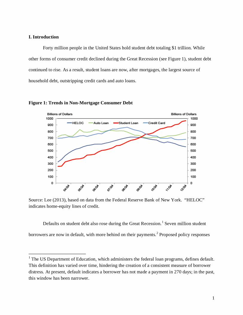
Forty million people in the United States hold student debt totaling $1 trillion. While

other forms of consumer credit declined during the Great Recession (see Figure 1), student debt

continued to rise. As a result, student loans are now, after mortgages, the largest source of

household debt, outstripping credit cards and auto loans.

Figure 1: Trends in Non-Mortgage Consumer Debt

Source: Lee (2013), based on data from the Federal Reserve Bank of New York. “HELOC” indicates home-equity lines of credit.

Defaults on student debt also rose during the Great Recession.1 Seven million student

borrowers are now in default, with more behind on their payments.2 Proposed policy responses

1 The US Department of Education, which administers the federal loan programs, defines default. This definition has varied over time, hindering the creation of a consistent measure of borrower distress. At present, default indicates a borrower has not made a payment in 270 days; in the past, this window has been narrower.

1

have included reductions in interest rates, forgiveness of student debt, more flexible repayment

plans and increased regulation of college prices. In the latest effort to respond to widespread

policy concern that there is a student debt crisis, President Obama signed in June 2014 an

executive order expanding eligibility for the Pay As You Earn program, which offers reduced

payments to borrowers in financial distress.

In this paper, I provide an economic perspective on policy issues related to student debt

in the United States. I begin by laying out the economic rationale for government provision of

student loans. I show time trends in student borrowing and describe the structure of the US loan

market, which is a joint venture of the public and private sectors. I then turn to three topics that

are central to the policy discussion of student loans: whether there is a student debt crisis, the

costs and benefits of interest subsidies, and the suitability of an income-based repayment system

for the US. I close with a discussion of the gaps in the data required to fully analyze and steer

student-loan policy.

To preview, I argue that there is no debt crisis: student debt levels are not large relative

to the estimated payoff to a college education in the US. Rather, there is a repayment crisis, with

student loans paid when borrowers’ earnings are lowest and most variable (Dynarski and

Kreisman, 2013). As a result, there is a mismatch in the timing of the arrival of the benefits of

college and its costs. Ironically, this mismatch is the very motivation for providing student loans

in the first place.

2 There were 6.5 million borrowers in default as of the third quarter of 2013. See http://studentaid.ed.gov/sites/default/files/fsawg/datacenter/library/PortfoliobyLoanStatus.xls.

2

One solution is an income-based-repayment structure for student loans, with a longer

window for repayment than the ten years that is currently the standard. While there exist income-

based repayment options within the current system, few borrowers take them up. The

administrative barriers to accessing these options are considerable, which may explain the low

take-up rate. Further, the existing options do not adjust loan payments quickly enough to respond

to the high-frequency shocks that characterize young people’s earnings, especially during a

recession.

A well-structured repayment program would insure borrowers against both micro and

macro shocks. With an interest rate that appropriately accounts for the government’s borrowing

and administrative costs, as well as default risk, this program could be self-sustaining. Designing

such a program requires detailed data on individual earnings and borrowing, which are currently

unavailable to researchers within and outside the government. If loan policy is to be firmly

grounded in research, this gap in the data needs to be closed.

II. The Economic Rationale for Government Loans to Students

Education is an investment. Like all investments, education creates costs in the present

but delivers benefits in the future. While students are in in school, expenses include both direct

costs (tuition, books) and opportunity costs. Future benefits include increased earnings, improved

health and longer life. To pay the current costs of their education, students need liquidity. In a

business deal, a borrower would put up collateral in order to fund a potentially profitable

investment. The collateral would typically include any capital goods used in the fledging

enterprise, such as a building or machinery. Similarly, homeowners put up their home as

collateral when they take out a mortgage.

3

Students cannot put themselves up for collateral: they cannot contractually commit to

hand over their future labor to a lender in exchange for upfront cash, because indentured

servitude is illegal. This is a market failure—there are good investments to be made, but private

lenders cannot or are reluctant to make these loans, just as they are reluctant to make (and

therefore demand higher interest rates for) other unsecured loans, such as credit cards. This

market failure explains why governments play an important role in lending for education. While

there have been occasional efforts to offer loans securitized by human capital (e.g., My Rich

Uncle), none has moved beyond a small niche market. Indeed, the public sector of most

developed countries and many developing countries provide loans to students.3

Given their prevalence, there is remarkably little compelling evidence of the effect of

student loans on educational investments.4 Students choose to borrow, so estimating the effect of

loans on outcomes is challenging: those who borrow likely differ from non-borrowers in ways

that will bias naive comparisons of their educational attainment. A randomized trial would solve

the selection problem, but there has been no experiment in which access to student loans is

randomly manipulated.5

The best observational evidence comes from South Africa and Chile (Solis, 2012;

Gurgand, et al, 2011). In these countries, students are offered loans only if they have a minimum

credit score (South Africa) or test score (Chile). The papers that analyze these loan programs

compare the college attendance of students right above and below these cutoffs, capturing the

3 In part, this is because it is very difficult for private parties to place a lien on (or confirm) individual earnings. By contrast, governments, through the income tax system, have the ability to both measure and collect from income. 4 See Dynarski and Scott-Clayton (2013) for a review of this evidence.

5 Field (2009) studies an experiment in which loan-repayment terms were randomly varied at a law school.

4

causal impact of loan availability. This research approach is referred to as “regression-

discontinuity” design. In a well-designed regression-discontinuity study, that it is essentially

random that someone ends up right above or right below the eligibility cutoff. A comparison of

these two groups therefore yields a causal estimate of the effect of program eligibility.

In Chile, right below the eligibility cutoff, 20 percent of students go to college. Right

above, the figure is 40 percent. The difference — 20 percentage points — is the estimated causal

effect of loan availability on college attendance for these students. The South African study

reaches a similar conclusion. Right below the credit-score cutoff, 50 percent of students go to

college, compared with 70 percent right above. Again, the estimated effect is a 20-percentage-

point increase in college attendance. These are large effects, indicating that student loans make

college possible for many students, at least in these two countries. While we would prefer to

have evidence from the United States, these studies currently constitute the best available

evidence on the causal impact of student loans on educational attainment.

III. Trends in Student Borrowing

As noted earlier, the stock of outstanding student debt now exceeds $1 trillion. The flow

of debt has also increased, with annual borrowing doubling between 2001 and 2011 (from

$56 billion to $113 billion, in constant 2011 dollars).6 Borrowing has increased, in part, because

there are more students: college enrollment rose 32 percent in the decade between 2001 and

2011.

6 See Figure 6 in College Board (2012).

5

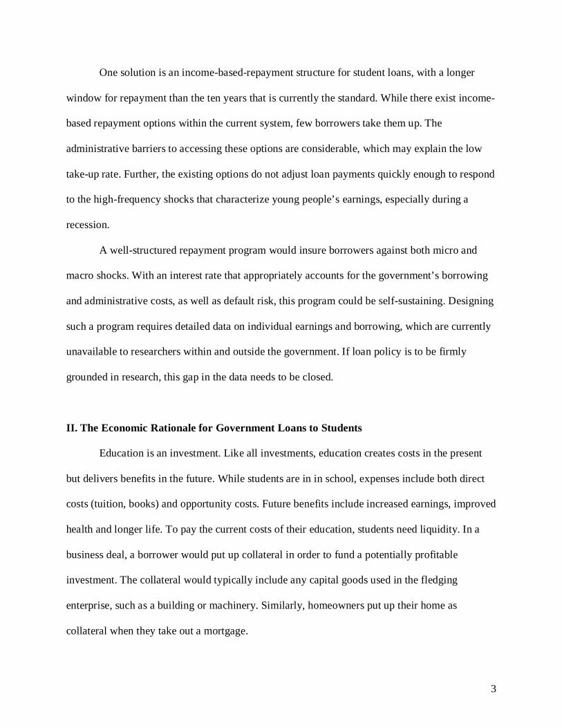
Figure 2: Aid per Full-Time-Equivalent Student

Source: College Board (2013), Figure 1.

But as the number of students increased, so too did annual borrowing per student, rising from

$3,500 to $5,400, an increase of 54 percent. 7 This per-student increase in borrowing can be

explained by one or both of two factors: an increase in the share of students taking out loans

and/or an increase in the size of the loans borrowers take out. Both of these factors appear to be

at work over the past decade. As discussed later in the paper, federal Stafford loans are the

largest loan program, accounting for 75 percent of student-loan volume (labeled as unsubsidized

7 Total fall enrollment (undergraduate and graduate) rose from 15.9 to 21.0 million between 2001 and 2011. See Table 221 in US Department of Education (2012).

6

and subsidized federal loans in Figure 2). In 2001 34 percent of undergraduates took out a

Stafford loan; by 2011 that number had risen to 50 percent.8 The average loan taken out by each

borrower went up by only 8 percent, by contrast—from $7,600 to $8,200, in constant 2011

dollars. The increases in the Stafford program, at least, are therefore on the extensive rather than

the intensive margin.

While we know that students now borrow more, the reasons are not well understood.

Rising college costs are a natural suspect. The sticker price of college has risen for years, but so

too has aid for college (see Figure 3). At public colleges, where 80 percent of students are

enrolled, the sticker price of college increased by $3,450 in real terms from 2001 to 2011. But

after netting out increases in grants and tax credits, the net price of college rose by just $1,160.

At private schools, which frequently offer grants to students, net prices rose even less, by $320.

These increases in net price cannot fully explain the $1,900 increase in average borrowing.

8 Besides Stafford, most other loans are also federal; just 7 percent of student loan volume was from private sources in 2011-12. PLUS loans to parents are the second-largest source of student borrowing (10 percent of volume), followed by PLUS loans to graduate students (6 percent). See Figure 6 in College Board (2012). The private and parental PLUS loans require a credit check or cosigner and so, as discussed earlier, are not classic student loans, which are secured only by the future earnings of the borrower.

7

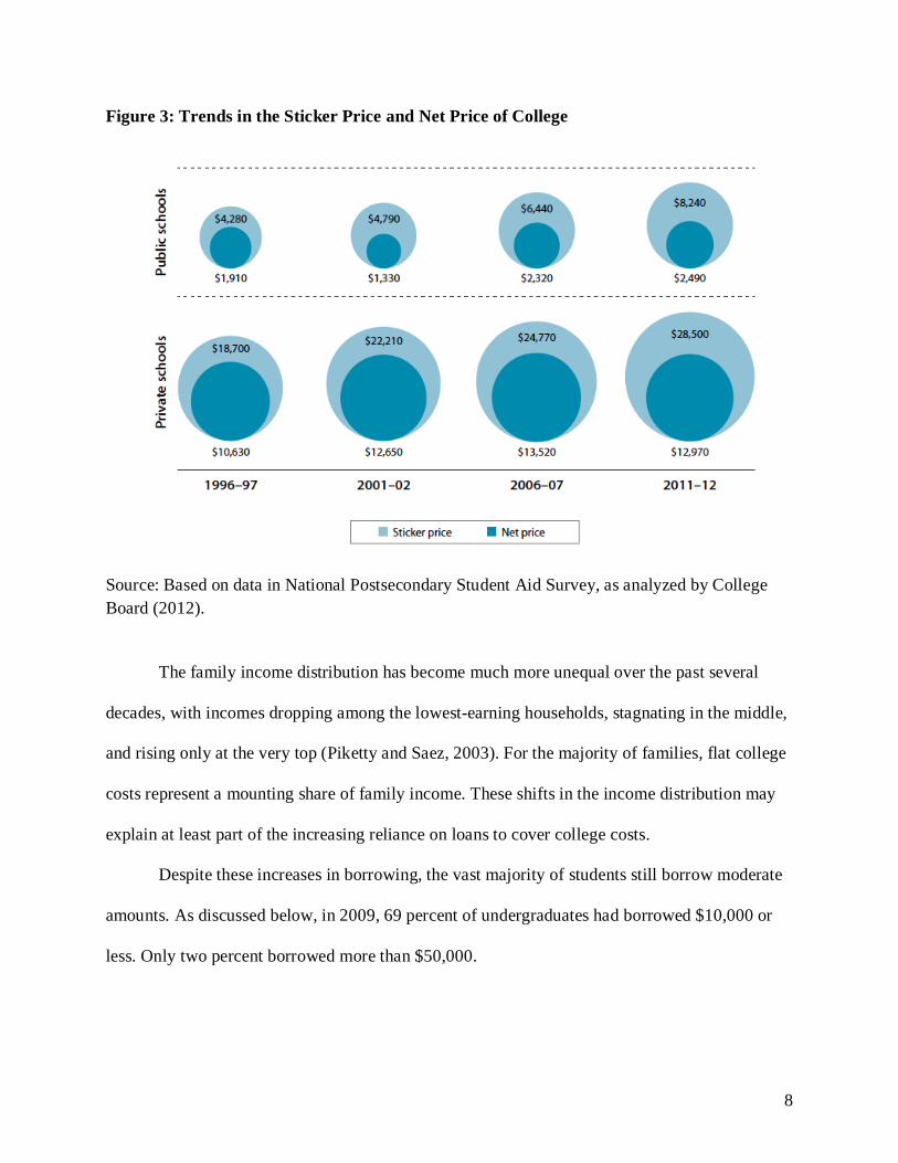
Figure 3: Trends in the Sticker Price and Net Price of College

Source: Based on data in National Postsecondary Student Aid Survey, as analyzed by College Board (2012).

The family income distribution has become much more unequal over the past several

decades, with incomes dropping among the lowest-earning households, stagnating in the middle,

and rising only at the very top (Piketty and Saez, 2003). For the majority of families, flat college

costs represent a mounting share of family income. These shifts in the income distribution may

explain at least part of the increasing reliance on loans to cover college costs.

Despite these increases in borrowing, the vast majority of students still borrow moderate

amounts. As discussed below, in 2009, 69 percent of undergraduates had borrowed $10,000 or

less. Only two percent borrowed more than $50,000.

8

IV. Students Loans in the US are A Public-Private Venture

The modern student loan program dates to 1965, when the Guaranteed Student Loan,

now known as the Stafford Loan, was initiated. From the start, federal student loans were a joint

venture of the public and private sectors. Private lenders provided capital, took applications,

disbursed loans and collected payments. The federal government defined eligibility for loans,

paid interest on some loans while students were enrolled in school, and guaranteed lenders

against default. Congress defined interest rates, loan maxima and other loan terms.

During the 1990s, the federal government began offering Stafford loans without a private

intermediary through the Direct Loans program. Private lenders continued to offer Stafford

loans, side-by-side with the new Direct Loan program. Which program a student borrowed from

depended on the college she attended, since colleges opted into Direct Loans.

The participation of the private sector in the federal loan programs was substantially

scaled back in 2010. With the passage of the Health Care and Education Reconciliation Act, the

Federal Direct Loan Program became the sole source of federal student loans in the United

States. The private sector now participates in the Stafford program only as “servicers” for the

Department of Education, collecting payments, keeping records and communicating with

borrowers.

The shrunken private role in Stafford loans can be traced to two events. First, the

financial crisis paralyzed the secondary markets that provided liquidity for private lenders. Short

of capital, private lenders turned away applicants and delayed loan disbursements, throwing the

Stafford program into disarray. The Direct Loan program, whose liquidity relies on the

borrowing power of the federal government, was unaffected.

9

Second, scandals undermined the political capital of the private lenders, who had long

campaigned against the expansion of the Direct Loan program. Media coverage depicted private

lenders as bribing school officials in order to gain preferential access to their loan-seeking

students.

While private lenders no longer offers loans through the federal loan programs, they

market a product labeled “student loans.” These private loans comprised as much as ten percent

of annual borrowing in the last decade. The private loans differ from the Stafford loans in this

crucial dimension: they require a creditworthy borrower or cosigner. As discussed earlier,

Stafford loans are provided to students regardless of their creditworthiness and with no security:

Stafford loans are “secured” only by the future earnings of the student borrower. By contrast,

private student loans are extended only to borrowers who have a good credit record, or a

creditworthy consigner. Private student loans are essentially unsecured consumer credit, much

like credit cards or personal loans.9 Unlike these types of credit, however, private student loans

cannot be discharged in bankruptcy.

The terms of private loans are typically worse than on federal loans. For example, these

loans do not allow access to the Pay As You Earn program or other initiatives intended to ease

repayment, nor so they allow for forbearance. Private loans are particularly prevalent at for-profit

colleges, whose students are three times as likely as other undergraduates to hold private loans.10

9 Federal PLUS loans, which are made to the parents of college students, also require a minimum level of creditworthiness as defined by the US Department of Education.

10 This begs the question: why would anyone take out a private loan? One hypothesis is that demand is induced by schools that are trying to avoid sanctions from the federal government, which kicks out of the federal aid programs (including the Pell) any schools whose students default too frequently on their federal loans. Some of these schools (community colleges, in particular) have withdrawn altogether from the federal loan program, so that their students have no alternative to the private market. Other schools still formally participate in the federal

10

The public-private partnership in the provision of student loans is sometimes strained.

During the Great Recession, defaults on student loans spiked. The federal government introduced

a variety of repayment plans intended to reduce defaults, but relied on the private servicers to

move borrowers into these more forgiving payment plans. Borrowers trickled slowly into the

new plans, frustrating policymakers eager to reduce defaults. The Consumer Finance Protection

Bureau has documented that in many cases loan servicers are unresponsive to borrowers who

want to restructure their payments.11 This dynamic echoes that of the mortgage crisis, when the

Home Affordable Modification Program (HAMP) was launched to help borrowers struggling

with their mortgages. HAMP relied on mortgage servicers to move borrowers into the new

plans, but progress was slow. While the goal was for four million borrowers to enroll in HAMP,

1.3 million did so.12

Here we have a classic “principal-agent” problem, with the agent (the student loan

servicers) having little incentive to act in the best interests of the principal (the federal

government). Student loan servicers don’t have much incentive to prevent borrowers from

defaulting, because the servicers either don’t own the underlying loans or, if they do, face few

costs if a borrower defaults. Restructuring a borrower’s payments and preventing default requires

effort, and the beneficiary of this effort is the government and the student – not the servicer.

Carefully written contracts are required to make such relationships work well; an entire field of

economics, mechanism design, is devoted to studying these contracts. In some cases, if the

program, but may steer borrowers they perceive as poor risks toward the private loans rather than the public options. Another, related hypothesis is that students are poorly informed about their borrowing options. 11 http://files.consumerfinance.gov/f/201310_cfpb_student-loan-ombudsman-annual-report.pdf

12 http://www.treasury.gov/initiatives/financial-stability/reports/Documents/March%202014%20MHA%20Report%20Final.pdf

11

principal cannot get the incentives right, she should just do the job herself. In the present context,

that would mean the federal government collecting payments on the loans it makes.

V. Is There a Student Debt Crisis?

Student loan debt is lower than is widely perceived. Consider students who first enrolled in

college in 2003–04. Six years later, in 2009, 44 percent had borrowed nothing and another

25 percent had borrowed $10,000 or less (see Figure 4). That is, 69 percent of undergraduates

borrowed $10,000 or less. Another 29 percent had borrowed between $10,001 and $50,000. Only

2 percent had borrowed $50,001 or more. Based on limited data, today’s entering college

students appear to be on a similar path. While attention is focused on extreme cases, only a very

small share of undergraduate borrowers hold the $100,000 loans that dominate the headlines.

Using the Survey of Consumer Finances, a household survey, Akers and Chingos (2014) reach a

similar solution.

Figure 4: Total Borrowing Among Undergraduates First Entering College in 2003-04

12

Source: College Board (2012), based on data from the National Postsecondary Student Aid Survey. Borrowing is measured for the six years following first-time college entry.

While attention is focused on borrowers with high loan balances, most defaults occur on

much smaller loans. For a cohort of undergraduates who borrowed in 2005, the loan balance of

those in default was smaller than among those who paid without adverse event: $6,625 versus

$8,500.13 Looking to the entire loan portfolio, including graduate students, the average loan in

default is about $14,000, while the average loan not in default is $22,000.14 Furthermore, the

data indicate that more students experience temporary rough patches than default, but do not

default: the delinquency rate (being behind on payments for 60 to 120 days) is much higher than

the default rate. Most of these delinquent borrowers eventually manage to repay, but with

damaged credit histories.

Graduate students borrow more than undergraduates. In fact, much of the recent growth

in student debt is attributable to graduate borrowing. In recent years, 40 percent of federal loan

dollars were disbursed to graduate students.15 Even though graduate students’ loan balances are

much higher, their default rate is only 3 percent, compared to 21 percent among undergraduate

borrowers.

13 See Table A-6 in Institute for Higher Education Policy (2011). These numbers are based on a cohort of 1.7 million students who borrowed in 2005. The federal government does not make these statistics available. The authors of the cited study gathered data themselves from loan servicers.

14 Calculated from data in http://studentaid.ed.gov/sites/default/files/fsawg/datacenter/library/PortfoliobyLoanStatus.xls. There are 6.5 million borrowers in default as of the third quarter of 2013, representing $89.3 billion in loans.

15 These figures are from Delisle (2014) and are based on calculations from the National Postsecondary Student Aid Survey.

13

VI. The Costs and Benefits of Interest Rate Subsidies

Student loans correct a capital market failure: the private sector will not provide loans

that are secured only by a borrower’s future earnings. If enhanced liquidity were the only goal,

loans would be offered at a market rate, with interest capitalized into principal while the student

was in college. In the policy arena, it is frequently argued that low interest rates help students by

encouraging college attendance and making loan payments more manageable. While an interest

subsidy certainly reduces payments (which begin after students leave college), it is a blunt tool

for increasing schooling and reducing loan defaults.

In the federal loan program, the interest rate is set to zero during college for low-income

students; loans with this benefit are called “subsidized” loans. Assume for the moment that loans

are offered at the market rate, and so the in-school payment of interest is the only subsidy. If a

student borrows $1,000 in her freshman year at a real rate of four percent, spends four years in

college, and pays the loan off in ten years, the in-school subsidy saves her $200 over the life of

the loan, or 20 percent of its face value.

All borrowers pay interest on federal loans after leaving school. This interest rate is set by

Congress, varies across the federal loan programs and is a hot topic of debate. At times the rate

has been fixed in nominal terms, and generated large subsidies for borrowers. During the late

1970s and early 1980s, when interest rates on mortgages were in the double digits, the interest

rate on student loans was fixed at eight percent. As of today, interest rates on federal student

loans are tied to Treasury bills. The 2013 Student Loan Certainty Act links interest rates to the

Federal 10-year Treasury rate, plus a margin. For the 2013-14 academic year, interest rates were

14

3.86 percent for undergraduate Stafford loans and 5.41 percent for graduate loans.16 They are 80

basis points higher for the upcoming academic year. Note that rates do not float for a given loan

– rather, they differ by the year in which they loan is initiated but are then fixed over the life of a

loan.

Can subsidized interest rates increase college enrollment? A lower interest rate reduces

the lifetime costs of college, so a rational decision-maker would include this price subsidy in a

calculation of the lifetime, present-discounted value of schooling. However, the evidence from

behavioral economics suggests that tangible and salient incentives at the moment of decision-

making are most effective in changing behavior.17 Interest-rate subsidies are not tangible when

students are deciding whether to enroll in college: students are handed the same funds whether

the loan’s interest rate is two percent, four percent or ten percent. The salience of an interest

subsidy is an unsettled question; I know of no empirical study that estimates a causal relationship

between college enrollment and the interest rate charged on student loans. While a field

experiment would be most relevant for policy, even a lab experiment would reduce our

ignorance about how interest rates affect student decisions.

Can subsidized interest rates reduce loan defaults? Here the answer is more

straightforward. In a mortgage-style payment system, where payments are fixed at the beginning

of the payment period, a lower interest rate reduces the monthly payments required to cover

principal and interest. In this case, a lower interest rate will make loan payments more

manageable for marginal borrowers and thereby reduce defaults. However, an across-the-board

interest subsidy benefits every borrower, including those who have high earnings and no

16 http://www.staffordloan.com/stafford-loan-info/interest-rates.php

17 Dynarski and Scott-Clayton (2013) discuss this evidence.

15

difficulty repaying loans. An interest subsidy is therefore a poorly targeted (and expensive) tool

for reducing loan default in a mortgage-style repayment system. Tying payments to income, as

discussed in Section VII, is a more targeted mechanism for reducing default.

In an income-based repayment system (discussed in Section VII) payments are a fixed

percentage of income. The interest rate does not enter into the calculation of the monthly

payment and affects only the length of repayment. For a borrower with a given principal and

lifetime income, a lower rate will reduce the time required to pay off the loan. This subsidy

therefore arrives at the end of the repayment period: payments stop earlier than they would have

otherwise. In a twenty-year repayment plan, this would means that a borrower stops making

payments (for example) when she is 42 rather that at age 43. These are peak earning years, and

the risk of default in this period is likely to be relatively low; the effect of the subsidy on

reducing defaults is also likely to be low. Further, this early cessation of payments equally

benefits borrowers with very high incomes and those with typical incomes. An interest subsidy is

therefore a poorly targeted (and expensive) tool for reducing loan default in an income-based

repayment system.

VII. Income-Based Repayment Plans Align the Timing of the Costs and Benefits of College

A college education is an investment that pays off over many decades. Over a lifetime, the

typical college graduate earns several hundred thousand dollars more than a high school

graduate. For most types of borrowing, the life of a loan matches the life of the collateral.

However, under the current system, the standard repayment period for a student loan is ten years.

The mismatch between the timing of the costs and benefits of education is especially salient

among young borrowers, who are most likely to default. Among borrowers under 21, for

16

example, 28 percent default on their loan. The default rate drops sharply with age, to 18 percent

of those thirty to forty-four and 12 percent among those forty-five and older (Institute for Higher

Education Policy, 2011). This pattern of defaults matches the age profile of earnings. Earnings

are lowest in the years right after college, when borrowers pay their loans. Among those with at

least a BA, median earnings are $32,000 for those aged twenty-four to thirty, $48,000 for those

thirty-one to forty, and $50,000 among those forty-one through forty-eight.18

An income-based repayment system determines loan payments based on income.

Payments rise and fall with income, thereby reducing pressure on borrowers when they first

graduate college (and whenever earnings are low). There are income-based loan programs in

Australia, Chile, New Zealand, Thailand, and the United Kingdom. In the United Kingdom, for

instance, borrowers contribute 9 percent of any income that exceeds £21,000; any remaining

student-loan balance is forgiven after thirty years. These countries can be useful models as

policymakers explore switching to an income-based repayment schedule. Dynarski and

Kreisman (2013) describe one such model for the United States.

Policymakers can adjust the specific parameters of an income-based system to achieve

alternative goals. Indeed, there are many contribution schedules that will work, with the choices

affecting the length of payment, the level of payments, and the share of loans forgiven. A lower

contribution rate leads to a lower payment, a longer payment horizon, more interest paid by the

18 These statistics are from the 2012 March Current Population Survey (authors’ calculations) exclude full-time students but include former students who are out of the labor force or unemployed. The twenty-fifth percentiles for those with a BA are $14,000, $24,000, and $15,000, respectively. Among those with some college but no BA, median earnings are $24,000 for those aged twenty-four to thirty, $30,000 for those in their thirties, and $34,000 for those aged forty-one to forty-eight. The twenty-fifth percentiles for this group are $6,000, $15,000, and $12,000, respectively.

17

borrower, and more loans forgiven after twenty-five years. Higher contribution rates have the

opposite effects.

The Pay As You Earn program (PAYE), which Mr. Obama expanded in his June order,

theoretically holds payments to 10 percent of income. The key limitations of PAYE, as well as

all of the other income-based repayment plans in the US, are that they are not the default option

and payments don’t adjust automatically with earnings.

The default option for borrowers is a ten-year, mortgage-style, fixed payment. Borrowers

must proactively apply to the income-based programs and demonstrate financial distress before

being admitted. Eligibility must be renewed annually. As the theory and evidence of behavioral

economics has demonstrated, defaults matter and even small administrative hurdles can keep

people from making beneficial choices. The Consumer Financial Protection Bureau has

documented the difficulties that borrowers have in navigating this process.19 The number of

borrowers in these flexible repayment plans is much lower than the number in distress and

default, which is evidence that the current system isn’t working to insure borrowers against risk

Payments do not adjust automatically in the existing income-based payment programs.

They are based on the previous year’s income, and change only if the borrower submits evidence

that income has changed. This backward-looking approach does not deal with shocks to income

as they arrive. As a result, even a borrower enrolled in PAYE can see more than ten percent of

income consumed by loan payments, if her earnings drop while enrolled in the program. Or less

than ten percent of her income may go to payments, if her earnings rise.

To effectively buffer earnings shocks as they arrive, payments need to adjust dynamically

with earnings. Such a framework has been advanced by several policy organizations, as well as

19 http://files.consumerfinance.gov/f/201310_cfpb_student-loan-ombudsman-annual-report.pdf

18

legislation currently pending in the US Senate.20 How would such a system work in the United

States? Social Security is a good model. Workers in the US do little paperwork to make Social

Security contributions: they complete an initial W-4 form and the employer handles the rest.

Social Security contributions then automatically rise and fall with earnings. Loan payments can

be handled the same way.

Some states are already moving toward income-based repayment. Michigan has now

joined Oregon in proposing a “Pay It Forward” student lending system in which students pay no

tuition up front and pay back a fixed percentage of their income after college. This sounds very

similar to the income-based repayment system I describe above. However, a key distinction is

that in a Pay It Forward program a borrower contributes a fixed percentage of income for a fixed

number of years. The liability is not denominated in dollars, as in a standard loan, but as a fixed

number of payments. Economists call this a graduate tax –a tax on earnings for those who have

gone to college. It is called a tax, rather than a payment, because a borrower can’t buy her way

out of the liability. The borrower is taxed for 25 years, even if she has repaid the principal (plus

interest) after a few years.

In the proposed Pay It Forward systems, a graduate who does extremely well in the labor

market will end up repaying many times over the cost of her education, while one who does

poorly will pay much less. There is therefore cross-subsidization in this system, with the

“winners” paying some of the college costs of the “losers.” Economic theory suggests that loans

funded by a graduate tax won’t work because those expecting high earnings won’t participate.

This is a classic case of adverse selection – borrowers who would be subsidized participate while

those who would subsidize stay away. This is unsustainable, as without the high earners the

20 See Dynarski (2014) for a discussion of these proposals.

19

system does not get enough payments to cover tuition costs. Because of adverse selection

graduate tax can work only if participation is mandatory, with everyone forced into the

borrowing pool.

This is similar to the dynamic in insurance markets, which collapse if sick people buy

coverage and healthy ones go without. The young, healthy participants cross-subsidize the older,

sicker participants, just as high earners subsidize low earners in a (mandatory) graduate tax.

Neither the Oregon nor Michigan plan requires all borrowers to participate in their programs.

This suggests that the programs would be brought down by adverse selection.21

A minor change to Pay It Forward will maintain its positives (simplicity, insurance

against bad draws in the labor market) while eliminating the negative (unsustainability caused by

adverse selection). The change is this: denominate debt in dollars, and let borrowers pay off their

debt. If a student borrows $25,000 and earns enough that she has paid back the principal plus

interest after just ten years, she will stop paying into the program. If a borrower instead runs into

hard times and still owes money after 25 years, the balance is forgiven.

VIII. Data on Student Loans Are Incomplete

An evidence-based policy requires data. Data on student loans are remarkably thin, given

the size of this market. They are particularly inadequate for modeling and costing out income-

based repayment plans. Understanding the relationship between individual earnings and

borrowing is critical for designing sound loan policy. If many former students carry debt beyond

their capacity to repay, policymakers need to reconsider the parameters of student borrowing,

21 Yale attempted a graduate tax in the 1970s, lending money to its undergraduates and then having them pay back a fixed percentage of their income for a fixed number of years. The program collapsed, with Yale ultimately forgiving outstanding debt.

20

such as eligibility, loan limits, loan forgiveness, and repayment structures. All of these topics are

currently under discussion in Washington, with little data to inform the debate.

To calculate the costs of an income-based repayment program, which typically includes a

forgiveness provision after a certain number of years, we need to know about borrowers’ lifetime

earnings. Many data sources contain information on lifetime earnings. There are also

comprehensive administrative data on borrowing through the federal loan programs. The two

have not been linked, however, which leaves analysts unable to examine the covariance between

lifetime earnings and borrowing. This is a critical parameter for designing a sustainable income-

based repayment system.

An example will demonstrate the necessity of individual-level data on earnings and

borrowing. The default rate on small loans is higher than that on large loans: the average loan in

default is $14,000 while the average loan in good standing is $22,000.22 This pattern of defaults

is consistent with two scenarios with very different implications for policy.

One scenario is that defaulters have temporarily low earnings and their loans fall into

distress during these unusual bad times. At low cost to government, an income-based repayment

program would insure borrowers against these temporary downturns by automatically reducing

their payments. If lifetime earnings are sufficient to pay off the loans, this system can be self-

funding.

An alternative scenario is that those who default have permanently low earnings that

cannot support even moderate debt loads. An income-based repayment plan would still help

these borrowers, but the ultimate cost to government would be much higher, since many of these

22 Calculated from data in spreadsheet “Direct Loan and Federal Family Education Loan Portfolio by Loan Status,” accessed October 2013. http://studentaid.ed.gov/sites/default/files/fsawg/datacenter/library/PortfoliobyLoanStatus.xls

21

loans will ultimately be forgiven. The cost of making, servicing and forgiving these loans could

be so high that a grant program could be cheaper for taxpayers.

Distinguishing between these two scenarios requires individual-level, longitudinal data

on student borrowing and earnings that follows former students for twenty-five years after

college. Why twenty-five years? Income-based repayment plans have students paying back their

loans 20 to 25 years, when any remaining balance is forgiven. Costing out these programs

therefore requires tracking earnings for decades. Why individual-level, longitudinal data?

Individual-level data are needed to capture the shocks to income that income-based repayment

programs insure against. The payments required of borrowers with different earnings paths

cannot be backed out from group averages. Any analysis that relies on averages will smooth

away the within-person shocks that are needed to estimate the benefits and costs of income-based

repayment.

How could this gap in the data be filled? The longitudinal surveys fielded by the US

Department of Education’s National Center for Educational Statistics (NCES) contain partial

information on borrowing and earnings. They would be adequate for the task of guiding loan

policy were they supplemented with administrative data.

The decadal NCES cohort surveys, which follow a high school class every ten years,

follow respondents only to early adulthood, typically stopping when respondents are in their

22

twenties.23 The postsecondary surveys (fielded about every five years) stop following

respondents about ten years after the start of college.24

To extend the borrowing data available for these surveys, they could be linked to the

National Student Loan Data System (NSLDS), an administrative data set that contains all federal

student loans. These links would be updated annually; they are currently updated only a couple

of times during the life of the surveys.

To extend the earnings data available for these samples, they could be linked to

administrative data from the Social Security Administration (SSA) or Internal Revenue Service

(IRS):

• SSA maintains longitudinal records of individual earnings. These records are used to compute Social Security benefits, which, like income-based student-loan repayments, are a function of lifetime earnings. Researchers have successfully linked SSA data to surveys, including the Census (an example is Angrist, Chen, and Song, 2011).

• IRS maintains household-level records of income-tax returns and the informational

returns that are used in the calculation of taxes. These data include information on college attendance, in the form of the 1098-T, which colleges send to the IRS to document tuition payments. In recent years, versions of these data have become available to outside researchers (e.g., Chetty et al., 2011). Treasury employees can

23 The National Longitudinal Survey of the High School Class of 1972 surveyed students until 1986, when they were about 32. High School and Beyond, which includes the high school class of 1982, stopped surveying students when they were in their twenties (in 1986, four years after high school). So did the National Education Longitudinal Study of 1988, which stopped surveying in 2000 (when respondents were about eight years out high school). The surveys currently in the field (Education Longitudinal Study of 2002 and the High School Longitudinal Study of 2009) are not planned to survey any later in life than their predecessors. See http://nces.ed.gov/surveys/hsb.

24 The Baccalaureate and Beyond has varied in how long it tracks students. Graduates who started college in 1993 were followed for ten years, which would yield a typical exit age of late twenties. See http://nces.ed.gov/surveys/b&b/about.asp.

23

also conduct research with these data, and outside researchers have coauthored with them on studies (e.g., Manoli and Turner, 2014).

The merged versions of these surveys with administrative data would, by necessity, contain

detailed, individual-level data from multiple government agencies. There are legal, political and

administrative barriers to creating and releasing such sensitive data, but they can be overcome.

The Census Bureau has been particularly aggressive and creative in matching administrative data

to its surveys and finding new ways to distribute those data to researchers, and could provide a

model for these purposes.

Census has linked its Survey of Income and Program Participation (SIPP) to data from

the Internal Revenue Service and made it available in its secure Research Data Centers, which

are located across the country and open to researchers who have undergone an extensive vetting

process. The downside of this model is that a very limited number of researchers gain access to

the data. A more promising approach is that taken by the SIPP Synthetic Beta.25 Through this

pilot project, Census publicly releases a version of its SIPP-SSA-IRS match that is “perturbed,”

with some variables statistically blurred to prevent identification. An unperturbed version of the

matched data sits on the Census servers. Researchers run and refine their statistical models on the

publicly available data, on their own computers. They can then upload the resulting code to the

Census servers, where it is run on the original, unperturbed data. Results are returned to the

researcher after being checked for compliance with data standards (e.g., minimum cell sizes).

The SIPP Synthetic Beta is a promising model for NCES to distribute versions of its data

that include variables sufficiently detailed that they threaten to reveal individual identities. This

25 See http://www.census.gov/programs-surveys/sipp/methodology/sipp-synthetic-beta-data-product.html for more information.

24

model could be used as the standard for merges of NCES surveys with sensitive data from IRS

and SSA. Agencies reluctant to allow their data to be released to researchers may well cooperate

when the SIPP Synthetic model is used, with public versions being statistically perturbed. This

approach appears to have worked with IRS and SSA, agencies that are notoriously protective of

their data.

IX. Conclusion

In this paper, I provide an economic perspective on student debt in the United States.

Governments across the world provide student loans, allowing students to borrow against the

lifetime welfare gains created by a college education. While borrowing has risen over time in the

US, so too has the return to schooling. The typical student holds debt that is well below the

lifetime benefits of a college education. The typical student borrower is not “under water,” as

were many homeowners during the mortgage crisis.

Rather, there is a mismatch in the timing of the arrival of the benefits of college and its

costs, with payments due when earnings are lowest and most variable. Ironically, this mismatch

is the very motivation for providing student loans in the first place. One solution is an income-

based-repayment structure for student loans, with payments automatically flexing with earnings

over a longer horizon than the ten years that is currently standard.

There are income-based repayment options in the US, but the administrative barriers to

accessing them are considerable. Further, the existing options do not adjust loan payments

quickly enough to respond to the high-frequency shocks that characterize young people’s

earnings, especially during a recession.

25

A well-structured repayment program would insure borrowers against both micro and

macro shocks. With an interest rate that appropriately accounts for the government’s borrowing

and administrative costs, as well as default risk, this program could be self-sustaining. Designing

such a program requires detailed data on individual earnings and borrowing, which are currently

unavailable to researchers within and outside the government. If loan policy is to be firmly

grounded in research, this gap in the data must be closed.

References

Akers, Beth, and Matthew Chingos. 2014. “Is a Student Loan Crisis on the Horizon?” Brown Center on Education Policy, Brookings Institution.

Angrist, Joshua D., Stacey Chen and Jae Song. 2011. “Long-Term Consequences of Vietnam-

Era Conscription: New Estimates Using Social Security Data.” American Economic Review 101(3): 334-38.

Chetty, Raj, John Friedman, Nathaniel Hilger, Emmanuel Saez, Diane Whitmore-Schanzenbach,

and Danny Yagan. 2011. “How does your Kindergarten Classroom affect your Earnings? Evidence from Project Star.” The Quarterly Journal of Economics Vol. CXXVI November 2011, Issue 4.

College Board (2012). Trends in Student Aid 2012.

http://trends.collegeboard.org/sites/default/files/student-aid-2012-full-report-130201.pdf College Board (2013). Trends in Student Aid 2013.

http://trends.collegeboard.org/sites/default/files/student-aid-2013-full-report.pdf Delisle, Jason (2014). The Graduate Student Debt Review. Unpublished manuscript, New

America Foundation. http://newamerica.net/sites/newamerica.net/files/policydocs/GradStudentDebtReview-Delisle-Final.pdf

Dynarski, Susan (2014). “Finding Shock Absorbers for Student Debt.” June 15, 2014. New York

Times, p. BU8. Dynarski, Susan and Daniel Kreisman. 2013. “Loans for Educational Opportunity: Making

Borrowing Work for Today’s Students.” The Hamilton Project. http://www.brookings.edu/research/papers/2013/10/21-student-loans-dynarski

26

Dynarski, Susan and Judith Scott-Clayton, (2013). “Financial aid policy: lessons from research.” Future of Children, 23(1), 67-91.

Field, E. (2009). “Educational debt burden and career choice: evidence from a financial aid

experiment at NYU Law School.” American Economic Journal: Applied Economics, 1(1), 1-21.

Gurgand, M., Lorenceau, A., & Mélonio, T. (2011). “Student loans: liquidity constraint and

higher education in South Africa.” Agence Française de Développement Working Paper No. 117. Retrieved from http://papers.ssrn.com/sol3/papers.cfm?abstract_id=1969424.

Institute for Higher Education Policy (2011). Delinquency: the Untold Story of Student Loan

Borrowing.

Lee, Donghoon. (2013). “Household Debt and Credit: Student Debt.” Federal Reserve Bank of New York. http://www.newyorkfed.org/newsevents/mediaadvisory/2013/Lee022813.pdf

Manoli, Dayanand S. and Turner, Nicholas. 2014. “Cash-on-Hand and College Enrollment:

Evidence from Population Tax Data and Policy Nonlinearities.” NBER Working Paper 19836.

Piketty, Thomas, and Emmanuel Saez. 2003. “Income Inequality in the United States, 1913–

1998.” Quarterly Journal of Economics 118 (1), 2003, 1–39. Solis, Alex (2012). Credit access and college enrollment (Uppsala University Department of

Economics Working Paper No. 2013:12). Retrieved from http://alexsolis.webs.com/CreditAccessSolis_v3.pdf.

US Department of Education (2012). Digest of Education Statistics.

http://nces.ed.gov/pubs2014/2014015.pdf

27