an economic model for valuing recreational angling ... economic model for valuing recreational...
TRANSCRIPT

An Economic Model for ValuingRecreational Angling Resourcesin Michigan
John P. Hoehn, Theodore Tomasi, Frank Lupi, and Heng Z. Chen
Department of Agricultural EconomicsMichigan State University
Volume I: Main Report
December, 1996
Report Submitted to
Environmental Response DivisionMichigan Department of Environmental Quality
and
Fisheries DivisionMichigan Department of Natural Resources

An Economic Model for Valuing Recreational Angling Resources
in Michigan
Dr. John P. Hoehn (PI), Dr. Theodore Tomasi (PI), 1 2
Frank Lupi, and Dr. Heng Z. Chen1 1
Report Submitted to:
Environmental Response DivisionMichigan Department of Environmental Quality
and
Fisheries DivisionMichigan Department of Natural Resources
December 1996
Department of Agricultural Economics College of Marine Studies1 2
Michigan State University University of DelawareEast Lansing, MI 48824-1039 Newark, DE 19716
© 1996 by John P. Hoehn, Theodore Tomasi, Frank Lupi and Heng Z. Chen. All rights reserved. Readersmay make verbatim copies of this document for non-commercial purposes by any means provided that thiscopyright appears on all such versions.

iii
Table of Contents
Volume I: Main Report Page
List of Tables . . . . . . . . . . . . . . . . . . . . . . . . . . . . . . . . . . . . . . . . . . . . . . . . . . . . . . . . . . . . . . . . . . v
List of Figures . . . . . . . . . . . . . . . . . . . . . . . . . . . . . . . . . . . . . . . . . . . . . . . . . . . . . . . . . . . . . . . . . vi
List of Abbreviations . . . . . . . . . . . . . . . . . . . . . . . . . . . . . . . . . . . . . . . . . . . . . . . . . . . . . . . . . . vii
Mathematical Symbols . . . . . . . . . . . . . . . . . . . . . . . . . . . . . . . . . . . . . . . . . . . . . . . . . . . . . . . . viii
Acknowledgments . . . . . . . . . . . . . . . . . . . . . . . . . . . . . . . . . . . . . . . . . . . . . . . . . . . . . . . . . . . . . ix
Chapter 1 Overview of the Project . . . . . . . . . . . . . . . . . . . . . . . . . . . . . . . . . . . . . . . . . . 1
1.1 Background1.2 Uses of the MSU Model1.3 Overview of the Research Process and the Report
Chapter 2 Economic Value and Its Measurement . . . . . . . . . . . . . . . . . . . . . . . . . . . . 6
2.1 The Concept of Economic Value2.1.1 Money measures of value2.1.2 Willingness to pay and willingness to accept2.1.3 Compensatory resource restoration 2.1.4 Recreational use, direct use, and passive use values
2.2 Measurement of Value 2.2.1 The travel cost method2.2.2 Economic benefits versus economic impacts2.2.3. Valuing injuries using recreation demand2.2.4 Components of the travel cost model
Chapter 3 Random Utility Models . . . . . . . . . . . . . . . . . . . . . . . . . . . . . . . . . . . . . . . . . . 18
3.1 The Basic Choice Model3.2 Estimating the Choice Model3.3 Nested Models3.4 Welfare Estimation
3.4.1 WTP per trip3.4.2 Expected WTP3.4.3 Welfare measurement in the nested model3.4.4 Aggregation
3.5 Participation

iv
Chapter 4 The MSU Random Utility Model . . . . . . . . . . . . . . . . . . . . . . . . . . . . . . . . . 33
4.1 Model Structure4.1.1 Trip and site types4.1.2 Choice occasions4.1.3 Nesting structure
4.2 Variables4.2.1 Site Level Variables 4.2.2 Other levels of nesting4.2.3 Estimation
4.3 The Survey Data4.3.1 Survey overview4.3.2 The survey sample 4.3.3 The design of the survey 4.3.4 The analysis sample
4.4 Estimation Results4.5 Model Predictions Using the Baseline Data
4.5.1 Procedure for predicting trips4.5.2 Statewide predictions of trips4.5.3 Single day trips4.5.4 Multiple day trips4.5.5 County level predictions
Chapter 5 Welfare Measurement with the MSU Model . . . . . . . . . . . . . . . . . . . . . . 71
5.1 Using the Existing Model5.1.1 Inland lakes5.1.2 Great lakes and anadromous runs5.1.3 Rivers and streams5.1.4 The value of Great Lakes fish5.1.5 Resource based compensation
5.2 General Themes from Policy Scenarios5.3 Further Research
5.3.1 Additional variables5.3.2 Redefining sites5.3.3 Contingent behavior5.3.4 Technical extensions of the model
References . . . . . . . . . . . . . . . . . . . . . . . . . . . . . . . . . . . . . . . . . . . . . . . . . . . . . . . . . . . . . . . . . . . 93
Volume II: Technical Appendices
Appendix 1: Model Specification . . . . . . . . . . . . . . . . . . . . . . . . . . . . . . . . . . . . . . . . . . . . 97
Appendix 2: Survey of Michigan Anglers . . . . . . . . . . . . . . . . . . . . . . . . . . . . . . . . . . . 169
v
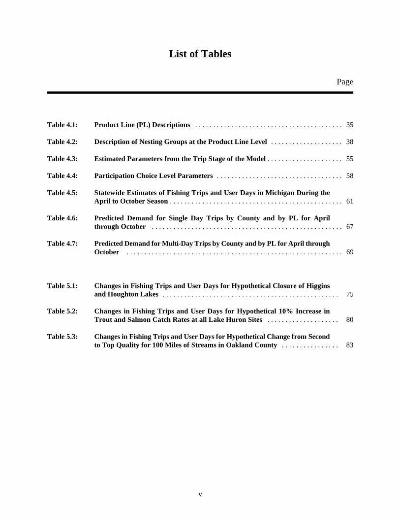
List of Tables
Page
Table 4.1: Product Line (PL) Descriptions . . . . . . . . . . . . . . . . . . . . . . . . . . . . . . . . . . . . . . . . . 35
Table 4.2: Description of Nesting Groups at the Product Line Level. . . . . . . . . . . . . . . . . . . . 38
Table 4.3: Estimated Parameters from the Trip Stage of the Model. . . . . . . . . . . . . . . . . . . . . 55
Table 4.4: Participation Choice Level Parameters. . . . . . . . . . . . . . . . . . . . . . . . . . . . . . . . . . . 58
Table 4.5: Statewide Estimates of Fishing Trips and User Days in Michigan During theApril to October Season. . . . . . . . . . . . . . . . . . . . . . . . . . . . . . . . . . . . . . . . . . . . . . . . 61
Table 4.6: Predicted Demand for Single Day Trips by County and by PL for Aprilthrough October . . . . . . . . . . . . . . . . . . . . . . . . . . . . . . . . . . . . . . . . . . . . . . . . . . . . . 67
Table 4.7: Predicted Demand for Multi-Day Trips by County and by PL for April throughOctober . . . . . . . . . . . . . . . . . . . . . . . . . . . . . . . . . . . . . . . . . . . . . . . . . . . . . . . . . . . . 69
Table 5.1: Changes in Fishing Trips and User Days for Hypothetical Closure of Higginsand Houghton Lakes . . . . . . . . . . . . . . . . . . . . . . . . . . . . . . . . . . . . . . . . . . . . . . . . . 75
Table 5.2: Changes in Fishing Trips and User Days for Hypothetical 10% Increase inTrout and Salmon Catch Rates at all Lake Huron Sites . . . . . . . . . . . . . . . . . . . . 80
Table 5.3: Changes in Fishing Trips and User Days for Hypothetical Change from Secondto Top Quality for 100 Miles of Streams in Oakland County . . . . . . . . . . . . . . . . 83

vi
List of Figures
Page
Figure 2.1: Travel Cost Demand Curve. . . . . . . . . . . . . . . . . . . . . . . . . . . . . . . . . . . . . . . . . . . . . 13
Figure 2.2: Consumer Surplus . . . . . . . . . . . . . . . . . . . . . . . . . . . . . . . . . . . . . . . . . . . . . . . . . . . 14
Figure 3.2: Hypothetical Nesting Structure for a Nested RUM. . . . . . . . . . . . . . . . . . . . . . . . . . 26
Figure 4.1: Four Level Nesting Structure for Each Choice Occasion: Participation, Trip,Product Line, and Site Levels . . . . . . . . . . . . . . . . . . . . . . . . . . . . . . . . . . . . . . . . . . . 40
Figure 4.2: Structure of Panel Interview . . . . . . . . . . . . . . . . . . . . . . . . . . . . . . . . . . . . . . . . . . 50
Figure 4.3: Trips and User Days by Type of Water Body . . . . . . . . . . . . . . . . . . . . . . . . . . . . . 61
Figure 4.4: Trips and User Days by Target Species Type . . . . . . . . . . . . . . . . . . . . . . . . . . . . . . 62
Figure 4.5: Michigan Population, Percent per County . . . . . . . . . . . . . . . . . . . . . . . . . . . . . . . . 62
Figure 4.6: Distribution of Predicted Single Day Trips . . . . . . . . . . . . . . . . . . . . . . . . . . . . . . . . 63
Figure 4.7: Distribution of Predicted Multiple Day Trips . . . . . . . . . . . . . . . . . . . . . . . . . . . . . . 65
Figure 5.1: IL Warm Single Day Trips under Roscommon Policy . . . . . . . . . . . . . . . . . . . . . . 76
Figure 5.2: IL Warm Multi-Day Trips under Roscommon Policy . . . . . . . . . . . . . . . . . . . . . . 77
Figure 5.3: Lake Huron Counties . . . . . . . . . . . . . . . . . . . . . . . . . . . . . . . . . . . . . . . . . . . . . . . . . 78
Figure 5.4: Single Day Trips under Oakland Policy . . . . . . . . . . . . . . . . . . . . . . . . . . . . . . . . . . 84
Figure 5.5: Multiple Day Trips under Oakland Policy . . . . . . . . . . . . . . . . . . . . . . . . . . . . . . . . 85
Figure 5.6: Michigan Counties . . . . . . . . . . . . . . . . . . . . . . . . . . . . . . . . . . . . . . . . . . . . . . . . . . . 96

vii
List of Abbreviations
Anad Anadromous run species of fish.CATI Computer assisted telephone interviewing.CERCLA Comprehensive Environmental Response, Compensation, and Liability Act.CR Catch rates for fish.DEQ Department of Environmental Quality.FIML Full information maximum likelihood estimation.GEV Generalized extreme value distribution.GL Great Lakes.IIA Independence of irrelevant alternatives.IL Inland lakes.IPPSR Institute of Public Policy and Social Research.IV Inclusive value.MDNR Michigan Department of Natural Resources.MERA Michigan Environmental Response Act.MSU Michigan State University.NOAA National Oceanic Atmospheric Administration.NRDA Natural Resource Damage Assessment.OPA Oil Pollution Act.Part 201 Part 201 (Environmental Response) of Natural Resources and Environmental Protection
Act, 1994 PA 451, As Amended -- Michigan.PCB's Polychlorinated biphenyls.PI Principal InvestigatorsPL Product line.RS Rivers and streams.RUM Random utility model.SRD Survey Research Division.SSI Survey Sampling Incorporated.SWTP Seasonal willingness to pay.TCM Travel cost method; travel cost model.WTA Willingness to accept.WTAR Willingness to accept in resources .WTP Willingness to pay.WTPR Willingness to pay in resources.

viii
Mathematical Symbols
(In order of appearance)
Y Income.P Price.Q Generic variable for environmental quality or fishing quality.V Utility; Conditional indirect utility.WTP$ Willingness to pay in dollars.WTA$ Willingness to accept in dollars.R Generic variable for resources; e.g., lake acreage.A Generic variable for species existence; e.g., anadromous species.WTAR Willingness to accept in resources. WTPR Willingness to pay in resources.S Generic variable for site characteristics; e.g., shoreline development.M Variable representing market goodsh Indicator for individuals (Chapter 3).A,B Indicator for two hypothetical sites, A and B (Chapter 3).� Parameters of the utility function.� Error term in RUM model; the unmeasured characteristics of individuals and sites;
"personalized term".K Some unspecified constant, a number represented by K.% Probability; % probability site A is visited; % probability of participating in recreation.A P
exp Represents the exponential function.* Summation operator.ln Natural logarithm.j,k Site indicator variables.X Vector of variables describing the characteristics of alternative j.j
L Set of available sites within a branch of a nested logit model.H,L Indicators for "high" and "low" values of some variable.IV Inclusive Value index; IV + constant equals the expected maximum conditional indirect
utility of some set of sites in a RUM model. D Akin to IV, but for nested logit models.T Number of choice occasions in a repeated logit model.W Generic variable capturing other variables at the participation level of a model.N Number of fishing trips or the expected number of trips.

ix
Acknowledgments
We are indebted to many individuals who have assisted and participated in this project. Brian Monroe,
our liaison in the Environmental Response Division of the Michigan Department of Environmental Quality,
was extremely helpful and accessible throughout the course of the research. Douglas B. Jester, Jr., our liaison
in the Fisheries Division of the Michigan Department of Natural Resources, provided valuable guidance and
actively participated in the development of the model. We are particularly grateful to Mr. Jester for sharing
his broad knowledge of Michigan anglers and fishing in Michigan, as well as his experience with previous data
collection and modelling efforts.
During the research process and the progress of the project the MSU team obtained feedback and
advice from an outside panel of experts. This panel included Dr. Richard Carson of the University of
California at San Diego, Dr. Michael Hanemann of the University of California at Berkeley, Dr. Edward Morey
of the University of Colorado, and Dr. George Parsons of the University of Delaware. The MSU team had
several meetings with the review panel as a whole and discussed matters with them individually at various
times. Their input and openness is appreciated.
During the course of the research, Dr. Carol Jones of the National Oceanic Atmospheric
Administration's Damage Assessment Center provided valuable comments and shared experience from similar
research in Michigan. In particular, we have made extensive use of the earlier model of fishing in Michigan
that Dr. Jones developed with Dr. Yusen Sung. In addition, Dr. Wiktor Adamowicz of the University of
Alberta and Dr. Douglass Shaw of the University of Nevada provided valuable comments during the course
of the research. We have also benefited from general conversations with Dr. Peter Feather of the United States
Department of Agriculture's Economic Research Service.
We thank all the individuals from the Survey Research Division of the Institute for Public Policy and
Social Research (IPPSR) at Michigan State University who worked on the survey. Dr. Jack Knott, Director
of IPPSR, and Dr. Larry Hembroff, Survey Director, were instrumental in keeping the survey on track. Ms.
Ning Na of IPPSR's Survey Research Division deserves recognition for managing the survey research. Special
thanks are owed to all the interviewers for their service and for their input and contributions during the survey
design phases.

x
Several colleagues at Michigan State University helped us to profile Michigan anglers and fishing in
Michigan including Dr. Douglas Krieger of the Department of Agricultural Economics, Drs. Jim Bence and
Shari Dann of the Department of Fisheries and Wildlife and Dr. Daniel Spotts of the Travel, Tourism, and
Recreation Resource Center. Drs. Jeffrey Wooldridge and Peter Schmidt of the Department of Economics
offered advice on econometric questions that arose over the course of the project.
We thank Tiffany Phagan for taking an interest in and making contributions to the project. Thomas
Moen provided excellent research assistance and deserves special recognition for his contributions to the policy
programs. Thanks are due to Chenfeng Lin and Jason Nolan who assisted with data management and
especially to Christian De Ritis for staying on to code all the fishing sites.
We thank our department chair, Dr. Lawrence Hamm, for his support of the project and his insights
into angling in Michigan. We are especially grateful to Nicole Alderman, Vicky Branstetter, and Janet Munn
of the Department of Agricultural Economics at MSU who have all helped to smooth and decode the
administrative aspects of the project.
While we have benefited from the insights and efforts of all of the above mentioned individuals, the
authors are solely responsible for the content of this report.

The project was established as Amendment Number 5 to an existing agreement between MSU and the1
Fisheries Division, MDNR. The funding was provided by the Environmental Response Division and theFisheries Division of MDNR. In 1995, the Environmental Response Division became part of the newlycreated Department of Environmental Quality (DEQ).
1
Chapter 1
Overview of the Project
1.1 Background
The Michigan Department of Natural Resources (MDNR) is responsible for protecting Michigan's
environment, conserving its natural resources, and providing outdoor opportunities for Michigan citizens
and visitors. In December 1992, the MDNR issued a grant to researchers at Michigan State University
(MSU) to investigate the economic value of the recreational angling in Michigan. The MSU team was1
charged with developing an economic model of recreational angling in Michigan which would help the
MDNR protect and manage Michigan's fishery resources.
This document is the projects' final report and has two volumes. This volume, Volume I,
describes the research approach, the model used, and the results obtained. It is intended to be meaningful
to those interested in the project and does not require expertise in economics and statistics. Volume II
of this report consists of two technical appendices, which provide detailed documentation of the model
and data.
The overall goal of the research was to build an economic model which can be used to:
(1) value recreational angling experiences in Michigan, and
(2) determine how the values for recreational angling are affected by changes in
water quality and other measures of fishing quality.
The MSU team determined that a statewide recreational angling demand model would be
appropriate for the project. The particular type of demand model employed is called a travel cost model
(TCM). A TCM model measures individuals' demand for fishing experiences, and the type of TCM
utilized for this project can examine how the value of angling experiences is affected by such factors as
the quality of the natural resource base.

The primary relevant federal statutes are the Federal Water Pollution Control Act (Clean Water Act; 332
U.S.C. § 1321(f)(4)&(5)), Comprehensive Environmental Response, Compensation, and Liability Act(CERCLA; 42 U.S.C. § 9607(f)), and the Oil Pollution Act (OPA; 33 U.S.C. § 2706). The relevant statestatute is Part 201, (Environmental Response) of Natural Resources and Environmental Protection Act, 1994PA 451 As Amended which supersedes the previous statute known as the Michigan Environmental ResponseAct (MERA).
2
The MDNR required that the design of the model and all procedures used in its implementation
be consistent with the highest quality standards of research practice in this field. Furthermore, the MDNR
indicated that the model might by applied in natural resource damage assessment (NRDA) under relevant
federal and state environmental laws and should be consistent with established NRDA guidelines.2
Therefore, the recreational angling demand model developed by the researchers (the MSU model) can
measure the economic value of changes in natural resource quality at a variety of sites. Likewise, state
personnel or a contractor may apply the MSU model to the valuation of environmental injuries in a
NRDA at a specific site.
1.2 Uses of the MSU Model
It is expected that the MSU model of recreational fishing demand will be useful to water and
fishery resource managers and for related policy analysis. Though the MSU model is primarily aimed
at establishing the value of recreational angling experiences, the MSU demand model can be used to
provide information on where and how often recreational anglers go fishing. Since the MSU model
relates the demand for recreational fishing to measures of fishing and water quality at various fishing sites
in Michigan, the model can be used to predict changes in fishing patterns resulting from changes in site
quality. In particular, the model can predict changes in total fishing trips statewide, as well as changes
in fishing trips in each county of Michigan. Further, the model can forecast changes in the mix of fishing
trips among alternative trip lengths, target species, and water body types. Coupled with information about
changes in the supply of fishing quality, the MSU model can also provide insight into the value (benefits
to anglers) of various management decisions. The value information is suitable for benefit-cost analysis
of projects that affect fishing and water resources. Examples of resource management decisions that
could benefit from the application of the MSU model include: fish stocking, predator and disease control,
angler access investments, license fees, impoundments, habitat rehabilitation, and pollution regulation
and control.

See note 2.3
3
An important anticipated use of the model and motivating factor for this research project is
NRDA. State and federal environmental statutes establish liability for harm to the environment caused
by releases of hazardous substances. The party or parties responsible for the release of hazardous3
substances into the environment are liable for damages associated with their activities. These damages
may include: (1) the cost of restoration, reparation, rehabilitation, and replacement of the harmed
resources, (2) compensation for the diminution in value of the harmed resources pending restoration/
reparation/rehabilitation/replacement, and (3) the reasonable cost of assessing damages. The MSU model
is directed at estimating a portion of the second element of damage. It is aimed at the economic use
values lost due to resource injury by a certain stratum of the general public; recreational anglers in
Michigan. In a NRDA research program, the MSU model can inform one element of an overall economic
damage assessment. This element is the damage pertaining to the use values associated with injured
recreational angling resources.
The first step in assessing natural resource damages resulting from a release of hazardous
substances is to determine the nature and extent of the injuries that have occurred. The next step is to
specify the nature and extent of the services provided by the resources, and how the injuries alter resource
service flows. Resource services provide benefits to people; they are things that people care about, such
as catch rates for fishing, varieties of bird species for birdwatching, visual amenities, or the knowledge
of the existence of the resource in a particular condition. In most circumstances, an economic model can
be designed to value a change in service flows. If altered service flows are linked to injuries, an economic
model of the value of service flows can be employed to estimate damages due to injuries at a specific site.
The current project specifies an economic model that can estimate the diminution in value of a
harmed resource pending restoration (lost interim use values) for several types of service flows affecting
recreational fishing in Michigan. This project is not directed at valuing any specific injury at any specific
site. In a particular NRDA effort, the State of Michigan or a contractor would need to specify the nature
and extent of the injuries and determine whether and how these could be linked to the MSU model on a
site-specific basis.
4
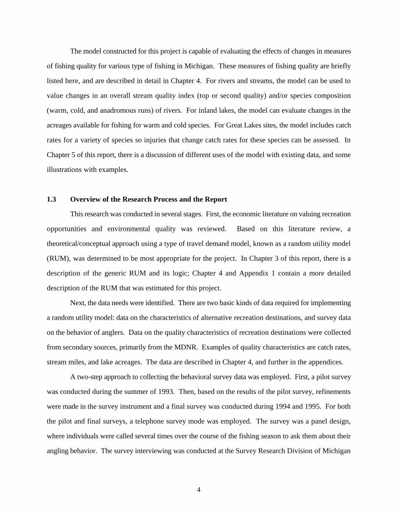
The model constructed for this project is capable of evaluating the effects of changes in measures
of fishing quality for various type of fishing in Michigan. These measures of fishing quality are briefly
listed here, and are described in detail in Chapter 4. For rivers and streams, the model can be used to
value changes in an overall stream quality index (top or second quality) and/or species composition
(warm, cold, and anadromous runs) of rivers. For inland lakes, the model can evaluate changes in the
acreages available for fishing for warm and cold species. For Great Lakes sites, the model includes catch
rates for a variety of species so injuries that change catch rates for these species can be assessed. In
Chapter 5 of this report, there is a discussion of different uses of the model with existing data, and some
illustrations with examples.
1.3 Overview of the Research Process and the Report
This research was conducted in several stages. First, the economic literature on valuing recreation
opportunities and environmental quality was reviewed. Based on this literature review, a
theoretical/conceptual approach using a type of travel demand model, known as a random utility model
(RUM), was determined to be most appropriate for the project. In Chapter 3 of this report, there is a
description of the generic RUM and its logic; Chapter 4 and Appendix 1 contain a more detailed
description of the RUM that was estimated for this project.
Next, the data needs were identified. There are two basic kinds of data required for implementing
a random utility model: data on the characteristics of alternative recreation destinations, and survey data
on the behavior of anglers. Data on the quality characteristics of recreation destinations were collected
from secondary sources, primarily from the MDNR. Examples of quality characteristics are catch rates,
stream miles, and lake acreages. The data are described in Chapter 4, and further in the appendices.
A two-step approach to collecting the behavioral survey data was employed. First, a pilot survey
was conducted during the summer of 1993. Then, based on the results of the pilot survey, refinements
were made in the survey instrument and a final survey was conducted during 1994 and 1995. For both
the pilot and final surveys, a telephone survey mode was employed. The survey was a panel design,
where individuals were called several times over the course of the fishing season to ask them about their
angling behavior. The survey interviewing was conducted at the Survey Research Division of Michigan

5
State University. The survey procedures are described briefly in Chapter 4. Detailed documentation of
survey procedures are contained in Appendix 2.
The next step in the research process was to estimate the parameters of the demand model using
statistical techniques. The basic logic and methods of the statistical approach is presented in Chapter 3
while detailed documentation is provided in Appendix 1. The estimated parameters of the model are
provided in Chapter 4 of the report. Chapter 4 also summarizes the model predictions for fishing trips
under baseline fishing quality conditions.
Based on the estimation results, the value of angling experiences, and/or the impact of pollution
events or management policies on angling values, can be determined. A non-technical description of
these values/impacts is contained in Chapter 3. The estimated welfare effects of some example changes
in service flows are contained in Chapter 5. The detailed implementation procedures used for computing
these welfare effects, including computer programs, are contained in Appendix 1.

6
Chapter 2
Economic Value and Its Measurement
This chapter of the report provides a brief overview of the economic concept of value that the
MSU model seeks to measure. There is a widespread conception that the value of something in the
economic sense is necessarily related to a market price. While value in general terminology has many
meanings, in mainstream economics value is precisely defined, and this definition need have nothing to
do with market prices. The basic concept of economic value is broader than the concept of a market, and
admits a wider array of measurement techniques than use of market prices. Non-market valuation
techniques allow the valuation of goods not traded on markets, such as recreation experiences and
environmental quality. Non-market measurement methods for values generated by recreational
experiences are described in this section, as are methods for determining the impact of environmental
quality changes on recreational values.
2.1 The Concept of Economic Value
Value theory begins by examining a person in a situation where he or she must make a choice and
the choice involves a trade-off, i.e., where something must be given up to obtain something else. The
logic of value theory can be applied to any object of choice. Objects of choice can be familiar market
goods, like shoes, or more complex goods, like school desegregation plans or ecosystems. What matters
is that people consider their options systematically, and choose the option they prefer. If one object is
chosen over another by a rational individual weighing his or her options carefully, it means that the
chosen object is at least as good (at least as valuable to the person) as what was given up. The value of
the chosen object can then be denominated in terms of the object given up. If what is given up is money,
then the value is measured in money terms. But the denomination need not be monetary; measurement
in some other unit of account makes the value obtained no less “economic.” What matters for calling a
value "economic" is that carefully considered trade-offs are being made by rational individuals.

7
2.1.1 Money measures of value
If a trade is denominated in money, the unit of account represents a general group of other,
unnamed goods. Money on its own holds no intrinsic value; willingness to give up (or get) money in an
exchange situation represents the willingness to forego (or obtain) the other goods one would purchase
with money. Which goods these would be depends on the person involved. What matters is the extra
well-being the person can obtain with a little more money, called the marginal utility of income.
The existence of an organized market for a good provides one context for making trades; it allows
people chances to make choices and for analysts to observe them. In a market economy (as opposed to
one using barter) observed trades are denominated in money. If a person is observed to pay $100 for a pair
of shoes, then one knows that the person is willing to give up $100 for the shoes. The $100 represents the
consumer's the ability to buy a collection of alternative goods. The opportunity to use the $100 in an
alternative manner is traded for the shoes, so the shoes must be worth at least $100 to that person. But
the $100 price for the shoes is only a lower bound for value since the person might be willing to pay much
more. The market here provides a convenient forum for observing choices and allows some information
about values to be inferred.
There are several relevant points to make regarding the economic theory of value. First, the theory
of value is specified at an individual level. There may be as many values for a good as there are people
valuing it. To define some sort of "social" value requires some method of aggregating individual values.
There is no one "correct" way to do this, and hence no "correct" social value of something -- though it is
common to aggregate values across people as a simple sum.
Second, there are no restrictions placed on why someone values a good. Economic values are
anthropocentric notions based on situations of rational choice. Third, the actual mechanism of choice can
vary, but it might be via a market, or it might be a negotiated explicit or implicit contract, or it might be
a public referendum.
Fourth, items that can be valued are broad, not just final consumption goods. Thus, an object may
have value because it produces something else of value. In this way, ecosystems and their elements might
generate value either directly (e.g., pleasure from canoeing in wetlands), or because they, like a machine,
generate something else that is valued directly (e.g., wetlands that are valued only for their provision of
flood control).

8
Fifth, values are not fixed and context-independent. Value will depend on the circumstances of
the trade presented to an individual. To decipher economic value, the economist ideally will know all the
attributes and circumstances of the trade-offs to be made: the (perceived) characteristics of the object of
choice, the good to be traded, the mechanism of the trade, and the and consequences of the trade. When
the analyst is unaware of some of the characteristics of the choice situation, he or she must make
assumptions about them. That, of course, is part of the challenge of the valuation task.
2.1.2 Willingness to pay and willingness to accept
There basically are two ways that choice situations arise: one in which people give up something
to obtain an object of choice (i.e., they pay for it) and one where they receive compensation in return for
giving up an object of choice (i.e., they sell it). Which side of the transaction individuals find themselves
on depends on the assignment of rights to the choice object. In the first case they do not have an assigned
right to the good, and they must pay to obtain it. In the second case they have an assigned right to the
good, and they must be compensated for giving it up.
The two alternative rights systems give rise to two concepts of value: willingness to pay (WTP)
and willingness to accept compensation (WTA). The former, of course, is constrained by what one brings
to the trade (e.g., income) as well as ones' tastes, while the latter is not constrained by individuals' incomes.
Hence, WTP and WTA are expected to differ, and the amount to which they diverge can be large. The
divergence between WTP and WTA depends upon (among other things) the ability to find a substitute for
the object you give up among the things you can get when you sell it (Hanemann 1993). If the object is
a unique natural resource with few good substitutes among goods you can buy with money, then its selling
price will be high, while its purchase price will be substantially lower.
The valuation research problem is to determine the smallest amount of compensation an individual
would require to sell a good, or the largest payment they would make to acquire it. A very simple model
can be used to illustrate the concepts. Suppose for the sake of argument that the ability to achieve a level
of economic well-being by an individual depends on three things: the amount of income they have, Y, the
prices of market goods they face, P, and the level of an index of environmental quality, Q. Under baseline
conditions, the index of environmental quality is at level Q , and the baseline level of well-being (called0

This notation V(x,y) can be read “V depends on the level of the variables x and y.” 4
9
utility) is V, and this can be written as V(P,Y,Q ). Now, suppose there is a release of some hazardous0 4
substance that reduces the index of environmental quality to a lower level, Q < Q . Then, the individual's1 0
well-being falls to the level
(1) V(P,Y,Q ) < V(P,Y,Q )1 0
That is, in (1), the individual is worse off (has a lower utility) with the release than without it.
Willingness to pay in dollars is the amount of money that could be paid, ex-ante, to avoid the
release. It is an amount of income, WTP$, that could be given up by the person and leave them no worse
off than they would be if the release had occurred. Thus, WTP$ is defined by the equation
(2) V(P,Y,Q ) = V(P,Y - WTP$,Q ) 1 0
Reducing income by the amount WTP$ and maintaining the baseline level of environmental quality leaves
the person just as well off as if the release had occurred, but they retained their income.
Willingness to accept compensation in dollars is given by an amount of income, WTA$, which,
if given to the person after the release, would restore them to the level of well-being they would had
achieved had to release never occurred. Thus, WTA$ is defined by
(3) V(P,Y + WTA$,Q ) = V(P,Y,Q )1 0
Because WTP and WTA are measures of the effects that a policy has on an individual's well-being, WTP
and WTA are referred to as welfare measures.
As discussed above, WTP$ does not generally equal WTA$. One circumstance in which these
alternative measures of value are equal is when the extra well-being that can be obtained from having more
income (the marginal utility if income) is a constant amount independent of the initial amount of income.
In this case, the utility function can be written as
(4) V(P,Y,Q) = �Y + f(P,Q),
10
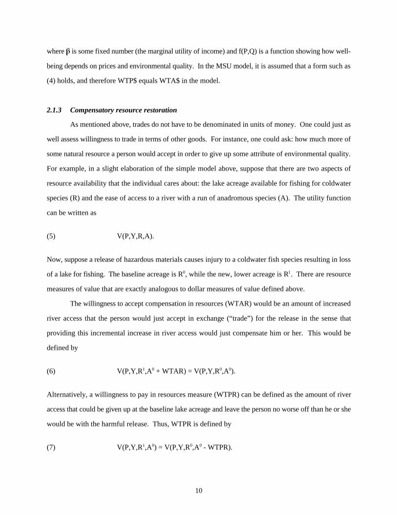
where � is some fixed number (the marginal utility of income) and f(P,Q) is a function showing how well-
being depends on prices and environmental quality. In the MSU model, it is assumed that a form such as
(4) holds, and therefore WTP$ equals WTA$ in the model.
2.1.3 Compensatory resource restoration
As mentioned above, trades do not have to be denominated in units of money. One could just as
well assess willingness to trade in terms of other goods. For instance, one could ask: how much more of
some natural resource a person would accept in order to give up some attribute of environmental quality.
For example, in a slight elaboration of the simple model above, suppose that there are two aspects of
resource availability that the individual cares about: the lake acreage available for fishing for coldwater
species (R) and the ease of access to a river with a run of anadromous species (A). The utility function
can be written as
(5) V(P,Y,R,A).
Now, suppose a release of hazardous materials causes injury to a coldwater fish species resulting in loss
of a lake for fishing. The baseline acreage is R , while the new, lower acreage is R . There are resource0 1
measures of value that are exactly analogous to dollar measures of value defined above.
The willingness to accept compensation in resources (WTAR) would be an amount of increased
river access that the person would just accept in exchange (“trade”) for the release in the sense that
providing this incremental increase in river access would just compensate him or her. This would be
defined by
(6) V(P,Y,R ,A + WTAR) = V(P,Y,R ,A ).1 0 0 0
Alternatively, a willingness to pay in resources measure (WTPR) can be defined as the amount of river
access that could be given up at the baseline lake acreage and leave the person no worse off than he or she
would be with the harmful release. Thus, WTPR is defined by
(7) V(P,Y,R ,A ) = V(P,Y,R ,A - WTPR).1 0 0 0
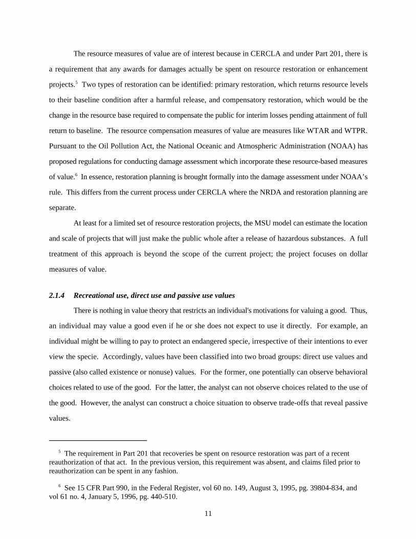
The requirement in Part 201 that recoveries be spent on resource restoration was part of a recent5
reauthorization of that act. In the previous version, this requirement was absent, and claims filed prior toreauthorization can be spent in any fashion.
See 15 CFR Part 990, in the Federal Register, vol 60 no. 149, August 3, 1995, pg. 39804-834, and6
vol 61 no. 4, January 5, 1996, pg. 440-510.
11
The resource measures of value are of interest because in CERCLA and under Part 201, there is
a requirement that any awards for damages actually be spent on resource restoration or enhancement
projects. Two types of restoration can be identified: primary restoration, which returns resource levels5
to their baseline condition after a harmful release, and compensatory restoration, which would be the
change in the resource base required to compensate the public for interim losses pending attainment of full
return to baseline. The resource compensation measures of value are measures like WTAR and WTPR.
Pursuant to the Oil Pollution Act, the National Oceanic and Atmospheric Administration (NOAA) has
proposed regulations for conducting damage assessment which incorporate these resource-based measures
of value. In essence, restoration planning is brought formally into the damage assessment under NOAA’s6
rule. This differs from the current process under CERCLA where the NRDA and restoration planning are
separate.
At least for a limited set of resource restoration projects, the MSU model can estimate the location
and scale of projects that will just make the public whole after a release of hazardous substances. A full
treatment of this approach is beyond the scope of the current project; the project focuses on dollar
measures of value.
2.1.4 Recreational use, direct use and passive use values
There is nothing in value theory that restricts an individual's motivations for valuing a good. Thus,
an individual may value a good even if he or she does not expect to use it directly. For example, an
individual might be willing to pay to protect an endangered specie, irrespective of their intentions to ever
view the specie. Accordingly, values have been classified into two broad groups: direct use values and
passive (also called existence or nonuse) values. For the former, one potentially can observe behavioral
choices related to use of the good. For the latter, the analyst can not observe choices related to the use of
the good. However, the analyst can construct a choice situation to observe trade-offs that reveal passive
values.

Since only dollar measures of damages are estimated on this project, WTP and WTA are used with7
the understanding that these are the dollar measures WTP$ and WTA$ defined earlier.
Here, the term consumer surplus is used in a generalized sense to refer to the exact Hicksian measures8
of welfare change defined earlier, WTP or WTA. The demand curves and areas under them referred tohere should be interpreted as Hicksian demands, not the usual Marshallian demands.
12
The notion of direct use has a history of being narrowly associated with on-site recreation
activities, typically associated with “user days” of an activity such as birdwatching, fishing, or hiking. In
fact, many direct uses will not be so closely related to on-site recreation. Individuals may have a number
of contacts with the resource base that would be direct use, yet such contacts would not measured by on-
site recreation value. For example, someone who lives near a river and crosses it as part of general travel
is engaged in a direct use relationship with the resource. This activity will not be counted as user days of
recreation, the value of which can be measured using a travel cost type model.
This project focuses only on the direct use values for recreational angling, measured in dollars.
Hence, it must be stressed that the model is intended to capture only a small portion of the values that
people attach to natural resources and environmental change.
2.2 Measurement of Value
There basically are two sets of ways to measure WTP or WTA. In the first, known as indirect7
or revealed preference methods, the analyst observes individuals' choices. The analyst then makes some
assumptions about the context of that choice, and infers a value from a model of choice. In the second,
known as direct methods, the analyst constructs a choice situation of known (to the analyst) design, places
people in this choice situation, and observes either a choice (as in an experiment) or a statement about what
choice would be made. Direct methods can be used to value either direct or passive use values, while
indirect methods can only be used to value direct use losses.
To value recreational angling opportunities, this project uses a type of indirect valuation approach
known as a travel cost model. Where and how often people go fishing is observed and used to infer the
value to them of alternative fishing opportunities. The travel cost approach is very closely associated with
the process of valuing goods that are traded on markets. The goal is to use market-like transactions to
estimate either the WTP or WTA concept of value. The measurement concept is called consumer surplus.8
Consumer surplus is an appropriate measure of value for any good for which a demand curve can be

13
Figure 1.1: Travel Cost Demand Curve
estimated. In the next section, the measurement of consumer surplus is illustrated in the recreation context
using a travel cost model.
2.2.1 The travel cost method
The travel cost method is a way of deriving the demand curve for recreational use of a natural
resource, such as fishing at a particular site. A demand curve is a relationship between the price of a good
and the quantity of the good purchased. In economics, it is generally assumed that the first unit of a good
is more highly valued than the n unit of the good. This concept is referred to as diminishing marginalth
utility. As a result, the demand curve will be downward sloping; that is, as the price of a good goes up,
all else constant, the quantity purchased will fall. The travel cost method seeks to derive the demand curve
by using travel costs as a proxy for the price of recreation.
To make this concrete, suppose that the good is fishing trips to Clear Lake. For this case, the
quantity consumed is the number of visits to Clear Lake over some period of time, such as a summer.
There is no market, and hence no market price, for fishing trips. However, the costs associated with travel
to and from Clear Lake function as the price for Clear Lake since an individual must decide whether to
incur travel and other access costs, when deciding whether to make a visit to Clear Lake. The costs
include the costs of travel (gasoline, lodging, and time) as well as any costs of gaining access to the lake
(parking fees, launch fees, etc.).
An example of a demand curve is
illustrated in Figure 2.1. On the vertical axis is the
cost of taking a trip, and on the horizontal axis is
the number of trips taken. The demand curve
shows the expected relationship of declining
number of visits as travel costs increase. The exact
position and shape of the demand curve will
depend on a number of factors, including the
person’s tastes for lake recreation, income, the
quality of the lake recreation site, including water
quality, and the location of (and hence travel costs to) and quality of alternative, substitute lakes to visit.

14
Figure 2.2: Consumer Surplus
For the Clear Lake example, the first fishing trip to Clear Lake is highly valued; the person is
willing to pay quite a lot in travel costs for this first visit. However, their willingness to pay in travel costs
per visit for the twentieth visit will be lower than it is for the first visit. This relationship is embodied in
the downward sloping demand curve. Consequently, if the person's travel cost to the lake is very high, say
a two hour drive costing $75, the person will make few visits to this lake, perhaps only twice per summer.
If the travel distance is short, say a fifteen-minute drive costing $10, the person will go relatively
frequently, perhaps twenty times over a summer. This is shown in Figure 2.1.
The essence of the travel cost method is to determine statistically the relationship between price
(travel cost) and quantity (number of visits) to the site. In applying the travel cost model to fishing, the
travel cost method is used to value the fishing experience at a specific site, not fishing in general.
The travel cost demand curve for trips
does double duty: it shows how many trips to the
site will be taken at a given price, and,
importantly, it also shows the amount this person
is just willing to pay to take a certain number of
trips per season to the site. By adding values for
all the trips taken to the site, the total willingness
to pay for trips to the site is obtained. In Figure
2.2, a demand curve is shown. When the travel
cost is TC, N trips are take to the site. The total
willingness to pay for the N trips is the area OABN (all the shaded areas in the figure). The amount
actually spent on travel is the price per trip times the number of trips, or $TC × N (the area OTCBN
labeled "expenditures").
Consumer surplus is the excess of total willingness to pay, over and above the amount that actually
was paid. This is the cross-hatched area TCAB. If Clear Lake was closed for the season, the loss of
economic well-being (economic value or economic welfare) for this person is measured by the consumer
surplus.
When employing the travel cost method to derive a demand curve, it is important to take into
account the availability of substitute fishing sites. If there are many good substitute lakes for Clear Lake,
In some cases, economic impacts can be measures of economic value. For example, if the relevant9
population is the people of Michigan, then changes in income brought to Michigan by nonresidents wouldbe a part of the measure of value change for Michiganders.
15
then a small increment in travel cost to Clear Lake will result in many fewer trips being taken there. In
this case the demand curve will be relatively flat and little consumer surplus will be generated.
Alternatively, if Clear Lake is relatively unique, an increment to access costs will have relatively little
impact on visitation. In this instance, the demand curve will be relatively steep and a great deal of
consumer surplus will exist. Therefore, to properly account for substitution possibilities, a model for any
one site really must be a model of choice among a variety of angling experiences at alternative
destinations. Such a model is described in Chapter 3.
2.2.2 Economic benefits versus economic impacts
The measure of loss in economic benefits from closing Clear Lake for the season is the consumer
surplus. To calculate this loss of benefits, the total amount spent traveling to the lake (OTCBN in Figure
2.2) is deducted from the total value of the lake (OABN) because when the lake is closed no travel takes
place and the money otherwise spent on travel is available to purchase other goods. The money lost in
travel expenditures is transferred elsewhere in the economy, and does not represent an overall loss of
value. The consumer surplus (the remaining area TCAB) represents the value to this person of being able
to go to Clear Lake as many times as desired at the travel price TC. The economic benefits (losses) that
are appropriate for measuring use values, WTA and WTP, are measured by consumer surplus.
Often, attention is devoted to the economic impacts of a change in policy or management (e.g.,
changes in jobs and income in local economies). The economic impacts are related to the expenditure
portion of Figure 2.2, represented by changes in the area OTCBN. While these impacts may be of interest
for some policy and planning purposes, they are not measures of economic value. Value estimates are
based on changes in consumer surplus, not in measures of economic impacts.9
Another point about economic benefits relates to benefit-cost analysis. Benefit-cost analysis
consists of comparing the benefits of a policy or program to its costs. As mentioned above, the benefits
of a policy which introduces a new recreation site are given by the consumer surplus for that site, not the
expenditures or economic impacts. However, many policies of interest will involve changes in the

16
consumer surplus of existing sites rather than creation or elimination of sites. For example, policy actions
are unlikely to eliminate fishing at all Great Lakes, though policies could affect the price or quality of
fishing at Great Lakes. In such cases, neither the total value of the resource, total consumer surplus, nor
the economic impacts are desired measures of benefits. The relevant measure of benefits (costs) is the
change in the consumer surplus that is associated with the policy.
2.2.3 Valuing injuries using recreation demand
The quality characteristics of the possible choices of places to fish are key determinants of the
demand for recreational fishing. Examples of quality characteristics are catch rates for various species,
shoreline development, and contamination in fish. If one of these characteristics is altered, the demand
for fishing trips to that site shifts, as does the demand at substitute fishing sites. In the earlier figures
depicting hypothetical demand curves, such a quality change results in a shift or movement of the entire
demand curve. For example, if the catch rate for a specie decreases at some site, the number of trips taken
to that site at any given price will likely decrease, though trips may increase at other sites. That is, the
decrease in quality would shift the demand curve for that site to the left.
When quality characteristics can be linked to injuries at a site resulting from a release of hazardous
substance, damages can be assessed using the travel cost method. For example, suppose that the demand
for recreational angling depends on, among other things, the catch rate of a fish specie at the site.
Suppose that a release of a toxic substance such as PCBs into the water at the site causes reduced
reproduction success, and hence reduced populations of fish. Suppose it can be determined what the catch
rate would be absent the release. Then, the travel cost method can be used to determine the extent to
which the demand for fishing at the site would shift with the increase in the quality of fishing at the site.
The change in consumer surplus for fishing at the site then measures the damages to recreational anglers
(lost use values) imposed by the PCBs.
More generally, when a quality change induces the demand curve to shift, consumer surplus
changes. Thus, when the travel cost demand curve can be linked to site quality characteristics, changes
in site quality can be valued by the change in consumer surplus for the recreation experience. In the case
of quality changes, the change in consumer surplus is given by the area between the two travel cost

Strictly speaking, this is true under a condition known as weak complementarity (see Mäler or Freeman).10
Weak complementarity holds between a market good and a public good if, when the market good is not beingconsumed, changes in provision of the public good do not change welfare. In the case of fishing, for example,the market good is travel to a recreation site, and the public good is water quality there. Weak complementarityholds if a person who does not travel to the site does not care about changes in water quality there.
17
demand curves for the site in question: one at the high level of quality, and one at the low level of
quality. 10
2.2.4 Components of the travel cost model
There are several components that are needed to implement a travel cost model. First, the
alternative activities and destinations available for fishing are identified. The relevant travel costs to these
alternative destinations are determined. These include both time and money costs of travel. Second, data
on the quality characteristics of alternative sites must be obtained. These data are used as variables in the
travel cost model, and they relate to the things that matter to anglers when they make choices among
alternative fishing sites and how often to fish at each site. The data on quality characteristics must be
available for all (or most) sites of interest, since it is the choice of one place among a set of alternatives
that is being assessed.
Third, data are obtained on the actual choices made by anglers. This is done by choosing a sample
of individuals and asking them (using a survey) about where they went and what they did on their fishing
trips.
Fourth, the analyst estimates the form of the demand relationship using the data he or she has
collected. Finally, the estimated demand relationships are used to obtain estimates of the value of fishing
sites, or of changes in the quality of fishing at those sites.

18
Chapter 3
Random Utility Models
The type of travel cost model implemented for this project is known as a random utility model
(RUM). The RUM was developed by McFadden (1974) and was first applied to recreation valuation by
Hanemann (1978). Since then, it has been used for valuing aspects of recreation by several investigators.
For a detailed description of the general approach, the reader is directed to descriptions of the RUM by
Morey and by Bockstael et al (1991). This chapter presents an intuitive description of the basic logic of
the RUM approach. More specific details about the RUM used for this project are provided in Chapter 4,
while the technical aspects of the model are provided in footnotes and Appendix 1.
The RUM model is especially useful and applicable when there are many alternative recreational
sites (i.e., fishing destinations). In such circumstances, any given angler will visit only one site on a given
choice occasion and over the course of a season will visit only a few sites. In other words, the observed
number of trips taken by any given angler will be zero for most sites. This is called a “generalized corner
solution.” While traditional demand models have been developed to estimate generalized corner solution
models, and could be applied in the travel cost framework, these approaches are most useful for data sets
where just a few goods (sites) are not consumed. In Michigan, there are hundreds of fishing sites and, for
any individual angler there will be hundreds of sites that are not visited. The RUM can accommodate this
type of data.
Moreover, the RUM is very useful in bringing a wide array of substitutes directly into the
derivation and estimation of the demand model. In particular, when a RUM model is used, the demand
for fishing at any site will be a function of the prices and qualities of all sites included in the analysis. As
discussed in Chapter 2, it is important to include relevant substitutes in the analysis if accurate value
estimates are to be obtained.
3.1 The Basic Choice Model
Suppose that one has information on where individuals go to fishing. Typically, anglers have
available a number of alternative destinations for fishing. Each possible choice of a destination represents

While the data include ice fishing trips, an ice fishing model in not estimated for this project.11
M is a composite commodity consumed with income not spent recreating. It is assumed that the relative12
prices of the components of this commodity do not change. Any other goods are assumed to be (weakly)separable from those consumed in the recreation “branch” of the utility function.
This is a conditional indirect utility function, defined for one choice occasion. It is conditional on the13
choice occasion and on the choice of site A. It is assumed that goods consumed across choice occasions areseparable from one another.
19
a combination of characteristics, such as the quality of the fishing at the site, as well as the price that must
be paid to get to the site (i.e., the site's travel cost). Observations about where anglers fish reveal
information about the trade-offs between travel costs (money) and site quality. That is, data on where
people go provide information on their willingness to trade income for site quality. This is the essence of
the model employed by the MSU team.
To begin the discussion of the basic model, divide the fishing season into small time periods,
called choice occasions. On a choice occasion, an angler can either make one fishing trip, or she can
decide to not go fishing. In the MSU model, choice occasions are ½ week intervals, of which there are
about 60 in Michigan's “open water” fishing season.11
Suppose that an individual gets utility (i.e., pleasure) from visiting a recreation site, denoted by
V, and that this utility depends on only two things: the quality characteristics of the site that gets visited
(call these Q, for fishing quality, and S, for shoreline development), and the amount of a market good that
can be consumed in addition to recreation (call this good M, for market). This is just for illustrative
purposes; people of course care about more than this. 12
Suppose further (again for illustrative purposes) that the utility of a visit to the recreation site (site
A) for individual (h) depends on the two measures of site quality (Q and S) and the market good (M) in
the following fashion:13
(8) V = � [M] + � [Q ] + � [S ] + �h,A1 2 A 3 A h,A.
The parameters � , � , and � are constants that describe the relative importance of the variables to h's1 2 3
overall utility. The parameter � is a fixed number that measures the contribution of consuming the good1
M to utility, while � and � measure the contribution of trip quality at recreation site A to h's utility.2 3
For example, suppose that Q is a measure of fishing success, such as the catch rate. Then, if the catch

This also could represent variations in perceptions of the characteristics of goods by individuals relative14
to the measured levels of these characteristics.
The error term may vary through time for individuals, so that the person does not always view the15
choices in the same way. It is assumed here that individuals know the value taken by their own error terms;it also is possible that there is a random component to choice.
20
rate is increased by one unit, the recreator's utility will increase by the amount � . Further, if she can2
consume one more unit of M, then utility goes up by � . If M is thought of as a composite good,1
representing all the other things the person can buy, then M is what is purchased with one's income and
� is the value of an increment to income. Thus, the ratio between these parameters (� /� ) gives us the1 2 1
relative value to the individual of catch rates for fish and income, or the dollar value of a one unit change
in catch rate.
It is assumed that all individuals have the same values for the � parameters. Individuals attachi
different utility values to trips to a site because people have different values for the variables included in
the model. There are two ways that individual variation can be accounted for. The first is by including
measured variables that act as demand shifters that vary across individuals, such as demographic
variables. Individuals with different values for these measured variables will have different demands.
The second way that individual variation enters the model is through the term � . This is an individual-h,A
specific term representing variation in tastes across the population. While M, Q , and S are observable,14A A
and the � parameters can be estimated statistically, the term � is not observable by investigators. �h,A h,A
is known by individuals when they make travel choices on any given occasion, but it is unknown to
analysts. Thus, it represents, in some sense, unavoidable errors introduced into the analysis since
researchers cannot know all the relevant aspects of every person’s decision problem.15
If the magnitude of the � parameters is known, a person's willingness to trade the quality of thei
recreation site for income could be assessed. That is, the value of a change in site quality could be
established.
3.2 Estimating the Choice Model
The goal is to estimate the parameters (i.e., � , � , and � ) of the utility function. This is done1 2 3
using statistical estimation procedures. The price index of the composite market good M can be set

Different people might experience the same quality attributes differently. For example, catch rates may16
be higher for those who know the lake. This is not considered in the MSU model which uses averages.Further, note that these are expected quality variables before the trip is taken; bad weather can lower catchrates, but this may not be known when it is decided where to go fishing.
21
arbitrarily, so set it at one. Let the travel cost of going to a site be given by P. The travel cost consists
of the money and time costs of gaining access to the site.
Suppose there are two sites available, A and B. These sites have qualities (Q ,S ) and (Q ,S )A A B B
and travel prices of P and P . Everyone who visits a site will experience the same quality attributes (atA B
least on average), but each will face a different travel cost, since people live in different places. The16
prices P and P are personalized prices. Note that in the MSU model there are many more sites than justA B
two.
A person has an amount of income (Y) that can be spent on fishing and on the market good. If
a person chooses to visit a site, the travel price must be paid. Then, the person is able to consume an
amount of the other good (M) equal to the available budget (Y), less the cost of the trip to the recreation
site (P). This residual budget, (Y-P), is the amount of income left over for buying M after paying for
recreating. Thus, if an individual chooses to go to site A, the person consumes the overall bundle: "a trip
to A with site quality (Q ,S ) and good M in the amount [Y-P ]." Similarly, if the person goes to B theyA A A
consume "(Q ,S ) and [Y-P ]." Thus, if the person goes to site A, the utility level that is achieved isB B B
(dropping the indicator h)
V = � [Y - P ] + � Q +� S + �A 1 A 2 A 3 A A
while if they go to site B, the utility level achieved is
V = � [Y - P ] + � Q + � S +�B 1 B 2 B 3 B B
Economic theory typically assumes that people choose among alternatives so as to maximize their
utility given their budget. Thus, they go to the site that they think gives them the most enjoyment;
otherwise, they would go somewhere else. Thus, a person will visit site A if
(9) V = � [Y - P ] + � Q +� > � [Y - P ] + � Q + � = V ,A 1 A 2 A A 1 B 2 B B B
The income Y is the budget allocated to this choice occasion which typically is not observable. Since17
the MSU model is specified as linear in income, the income term (� Y) drops out because is does not vary1
across alternatives. In a RUM, variables that are constant across all choices drop out, since only utilitydifferences matter for choice and estimation. The parameter � can be estimated because the price term (travel1
cost) varies across choices.
22
and they will visit site B if the inequality is reversed and site B gives them more enjoyment. The
inequality in (9) is exploited to estimate the parameters of the utility function (the �'s).
Survey methods can be used to obtain data on where people go fishing. In addition, the cost of
getting to the alternative fishing sites (the Ps), and the quality of the fishing at the sites (the Q's and S's)
can be determined. What remains unknown are the values of the parameters � , � , and � , and the error1 2 3
terms (�'s). To obtain these, statistical techniques are used to identify the combination of these17
parameters that makes it most likely to actually see the pattern of fishing visitation that is observed in the
behavioral data. For example, suppose that � is large and � is small; then this indicates that people care1 2
relatively more about income than catch rates. In this case, one would expect to see people staying close
to home and not driving really far to get to high quality sites. Conversely, if � is small and � is large,1 2
people care a lot about catch rates relative to money, and one would expect to see them incurring travel
costs (paying a high price) to avail themselves good fishing sites. Additionally, the different measures
of site attributes in Q and S play a role here; suppose that S is an index of whether there is contamination
at a site. Then, if people really care about contaminated sites and stay away from them, one would expect
� to be a negative number. 3
Overall, for any distribution of the error terms, there is one set of parameters that best reproduces the
observed pattern of behavior (i.e., the pattern of travel to sites with varying quality). These best parameters are
called the maximum likelihood estimates of the true parameters � , � , and � .1 2 3
The existence of the unobservable “error” term � makes the problem uncertain from the analyst's
viewpoint. Given the cost of getting to a site and its measured quality, the analyst can only calculate the
chance that any given individual will find it the best site and go there. This chance depends on how likely
it is that a particular value of � arises. Large values of � make a site more attractive while small or
negative values make a site less attractive.
The term � can take on one of any number of values, according to a statistical distribution; that
is, some values of � are more likely to be true than others. This is why the model is called a random
23
utility model. The statistical distribution used determines the type of RUM, and hence the type of travel
cost model. Details of the statistical theory of estimating these types of models can be found in Maddala;
Ben Akiva and Lerman; and the references cited therein. The computer routines for implementing the
MSU model estimation are provided in Appendix 1.
The important thing about taking account of the error term is that, from the analyst's viewpoint, there
is only a chance that any person will find a particular site the most attractive. Even with knowledge of the �'s,
the personalized terms (the �'s) are not observable. If someone has a very large � but a small � , then theyA B
may visit site A, even though B looks better simply in terms of measured characteristics (travel cost and site
quality). Thus, there is some chance that any person has a given ranking of sites, and therefore some chance
that they find any given site best. The statistical model, in addition to providing estimates of the �s, also
provides information on the individual's chances of visiting sites.
To illustrate this point, suppose that a number is picked for each of the � terms. Conditional on
these numbers being chosen, one can calculate which site is best, the site that provides maximal utility.
But remember that there is only a probability that these numbers are the true �'s; the true error terms might
be other numbers. Rearranging terms in the expression (9) above, the person will visit site A if
� - � > {� [Y-P ] + � Q + � S }- {� [Y-P ] + � Q + � S } = K. A B 1 A 2 A 3 A 1 B 2 B 3 A
The term on the right side of this inequality is, for given �'s, just a number, call it K. Then this
inequality says that if the random term (� - � ) exceeds this number K, then the person visits site A.A B
There is some chance that this person finds site A best, based on the statistical probability that (� - � )A B
exceeds this number K. This probability is inherent in the statistical distribution of � - � . This can beA B
expressed as
The probability Ais the best site (% ) V A = Probability { V > } A B
% = Prob { � - � > K }AA B
(10) % = Prob {� -� > [-� P +� Q +� S ]-[-� P +� Q +� S ] }AA B 1 A 2 A 3 A 1 B 2 B 3 B

In this case, the probability of visiting site j is exp[�X ]/ � exp [�X ] where V =�X +� .18j k k j j j
24
Note that the income term has dropped out of this equation. So too would any term that did not vary
across the choices. For example, if all sites have a fish consumption advisory, then one could not assess
the impact of such advisories. Only differences in utility across choices matter in this theory.
Once a statistical distribution for the error term � is selected, the �'s can be estimated, and the
chances that a person finds any particular site the best can be calculated. The model is slightly more
complicated if there are many sites, but the basic idea is the same; the inequality in (9) must hold for all
the other sites besides A if A is the best.
The form of the selected distribution for the error terms determines the type of RUM being
estimated. For example, if the error terms, �, are independent draws from an extreme value distribution,
then a simple logit model results. The extreme value distribution is one of many possible distributions.18
The relationships among random choice models, the types of choice probabilities, and the statistical
distribution chosen for the individual-specific terms � has been established by McFadden (1974, 1981).
The expression for the choice probabilities above, (10), states that an increase in any variable, like
Q , that raises the utility of visiting site A, raises the chance that site A is visited. These chances orA
probabilities of visiting a site can be thought of as the expected demand for fishing at the site. Further,
equation (10) makes it clear that the utility of visiting a site is being compared with the utilities of visiting
all the other sites. Thus, substitution among sites is directly incorporated into the model.
3.3 Nested Models
As discussed above, there is an intimate tie between the structure of the choice model and
assumptions about the form of the statistical distribution of the error terms, �. One approach, called the
simple logit model, assumes that the error terms have a Type 1 extreme value distribution and that each
� is an independent draw from this distribution. This treats all potential choices as equally close
substitutes for one another, with none systematically more similar than others. Technically, this is known
as the independence of irrelevant alternatives (IIA). The concept of independence means that knowledge
of the � for one choice tells us nothing about the magnitude of the � for any other choice. The limitations
of the IIA idea can be illustrated using a famous example from transportation choices.

The general form of the GEV distribution and its relationship to choice probabilities arising from random19
utility maximization and the IIA property is discussed by McFadden (1974, 1981), Morey, and Ben-Akiva andLerman. See also technical Appendix 1.
25
Suppose a person has available three ways to get to work: a red bus, a blue bus, and a bicycle.
Under the IIA assumption, the odds of choosing the red bus over the bicycle do not change if the blue bus
becomes available. But this seems unreasonable. Clearly, any personalized factor that makes it likely
to choose a red bus over a bicycle, also makes it likely that the blue bus would be chosen over a bicycle.
Thus, knowledge that � is large (relative to � ) provides information that � likely is large asred bus bicycle blue bus
well, contradicting the idea that these are independent of one another.
If it is thought that this IIA assumption is not a good one, that some choices are more similar than
others, and hence that correlation among the errors is important, there is a more general approach. It
comes from using a special case of the generalized extreme value (GEV) distribution, and is called a
"nested" RUM. This approach was developed by McFadden. 19
The nested version of the RUM divides the alternative choices into groups that are relatively more
similar with alternatives in the same group than with alternatives in different groups. For example, to an
angler interested in fishing for lake trout in the Great Lakes, all the Great Lake sites may be closer
substitutes for one another then a Great Lake site and an inland stream site would be. Similarly, for a
brook trout angler, two cold water stream sites may be better substitutes for one another than a stream site
and an inland lake site would be.
What is sought, then, are groups of choices where the IIA assumption holds within the group, but
not necessarily across groups. Hence, within each grouping of choices, the alternatives appear to be
equally good substitutes. For example, suppose all the Great Lakes fishing sites are one group, and all
the inland stream sites are another. Knowing that the � for fishing out of Muskegon (a Lake Michigan
site) is high for a person, makes it more likely that the � for fishing out of Ludington (another Lake
Michigan site) is high as well, at least compared to fishing on the Pigeon River.
To understand the estimation of a nested model, it is useful to think of an individual's decision
of where to go as taking place sequentially. In fact, such decisions do not necessarily take place in this
sequential manner, but this is a useful pedagogic device. Suppose that the structure of choice is as
follows: there are three types of fishing: Great Lakes (GL), inland lakes (IL), and rivers and streams

In the MSU model there are twenty-four types of fishing: twelve for day trips and twelve for20
multiple-day trips. See Section 4.1.3 for details.
The inclusive value index is given by IV = ln[� exp(�X )], where L is the set of sites available in a21j�L j
branch, and �X is the deterministic portion of the conditional indirect utility of visiting site j in L.j
26
Figure 3.2: Hypothetical Nesting Structure for a Nested RUM
(RS). Within each of these groups there are several alternative destinations, among which IIA holds.20
The angler can be thought of as first choosing which type of fishing to engage in, and then, having made
this choice, which specific site to visit. This decision structure can be pictured as in the Figure 3.1.
First, the angler chooses among the three basic types of fishing, and then, conditional on this
choice, chooses a site. When deciding among sites within a "branch" of the decision tree, say among GL
sites, an individual chooses the best available, exactly as described above for a non-nested model. But
how should the person choose from among the three "water body type" branches GL, IL, and RS? What
is needed is a summary variable which summarizes the choices available in each of the lower “branches”
of the decision “tree.” Such a summary variable is the “inclusive value index,” denoted by IV. There21
is one for each available branch; in this example, there would be one for the GL branch, one for the IL
branch, and one for the RS branch. The inclusive value index gives the expected value of the highest

The expected value of the maximum conditional indirect utility is the IV plus a constant. The constant22
drops out of measures of welfare changes, and in what follows, the constant term is ignored.
27
utility the person would achieve if they chose that branch, not knowing exactly which site they would
visit. The inclusive value index for GL "summarizes" that choice in the sense that it measures the22
maximum expected utility from fishing at any GL site. Similarly, the inclusive value indices for the IL
and RS branches summarize the expected maximum utility for sites in those branches. Then, choice
among the three water body types (branches) can be made based on the relative magnitudes of the
inclusive value index across water bodies, as well as other variables that influence this choice.
Just as with the non-nested RUM, analysts can not know all there is about people and the
characteristics of the choices they make. The � terms capture these idiosyncracies, both within and across
branches. Hence, there is some probability that the person chooses a particular site within a branch. For
example, one can estimate % -- the probability that an angler chooses the GL branch, and theGL,Muskegon
Muskegon site. This chance can be decomposed into the product of two terms: the chance of choosing
a GL site (% ) and the chance of choosing Muskegon, given that one is going Great Lakes fishingGL
(% ). Muskegon|GL
If some GL site is improved in quality, then the probability of visiting that site, given a GL choice
goes up. Moreover, the overall utility for GL fishing, given by the inclusive value index for the GL
branch, goes up as well. This, in turn, increases the probability of choosing Great Lakes fishing over
other types. There may be many levels of such branches. For example, the GL, IL, and RS groups
mentioned above may be further divided based on other characteristics of trips (e.g., trip duration) and/or
characteristics of sites (e.g., geographical region).
3.4 Welfare Estimation
This section of the report, discusses how the model and estimated parameters can be used to
determine WTP for a change in quality of recreation sites. First, there is an illustration of how to compute
WTP per trip when the statistical/random utility nature of the problem is ignored. Next, there is a
discussion of how to introduce this statistical uncertainty into the calculation of WTP per trip. This is
done for the case of a non-nested model, since the logic is easier to see in this case; the extension to
nested models is then briefly considered.
This derivation holds only if the site where quality changes remains the best site before and after a23
quality change. More generally, one seeks the reduction of income that would equate the indirect utility ofthe best site before a change in quality to the indirect utility of the best site after a change in quality. Thus,if the site where quality changes is not the best before or after the change, then there is no change in theindividual's well-being.
28
3.4.1 WTP per trip
This section addresses the issue of how the RUM model can be used to assess economic value for
environmental quality associated with recreation. Consider first the case without the inclusion of the
personalized � terms. Suppose that the quality of the environment declines at a site, from Q ("high"H
quality) to a lower value Q ("low" quality). Then, for an individual who visits that site before and afterL
the change, the value of V attained will fall as well; the person is worse off with Q . Let the measure SL
remain unchanged. In this case, the following inequality must hold
(11) V = � [Y-P] + � Q +� S > � [Y-P] + � Q +� S = V .H H L L1 2 3 1 2 3
Equation (11) says that, holding constant the consumption of other goods (where M = Y-P, i.e.,
consumption of other goods equals income less the expenditure on travel to the site), the initial level of
well-being, V , is higher than the level of well-being attained with a degraded environment, V . H L
To get willingness to pay to avoid this change in environmental quality, compute the amount of
income that could be taken from the person when the quality of environment is at the baseline level QH
to make them as well off as they would be when the environmental quality is at the low level Q , and theyL
have their base income. The individual is using a high-quality recreational good, with quality Q , butH
income is subtracted until they attain level of well-being with the degraded environment. Denote the
amount taken from income by WTP. This value of WTP satisfies
(12) � [Y-P - WTP] + � Q +� S = � [Y-P] + � Q + � S .1 2 3 1 2 3H L 23
Solving this equation for WTP, it can be seen that
(13) WTP = (� /� )[Q - Q ].2 1H L
The WTP in this case is the incremental value of the quality variable times the amount of quality change.
Therefore, if there were no error terms (�'s) and values of the � parameters were known, the WTP

Since estimates of parameters are random variables, WTP is a random variable. In fact, the expected value24
of WTP is not exactly equal to the ratio of the point estimates of the parameters; this is only true in the limitas the sample size becomes large. For small samples, one can use an approximation approach (Bockstael andStrand) or a Monte Carlo approach (Adamowicz et al. 1989a and 1989b; Graham-Tomasi et al.; Kling andSexton; Kling).
29
measure of welfare for an individual could be easily computed. Of course, the true values of the �
parameters are not known, but, as explained above, estimates of them can be obtained. An estimate of
WTP is then obtained by inserting the estimated �'s into formula (13) for WTP. 24
3.4.2 Expected WTP
That the model has a random component means that the true measure of WTP for any individual
is known only up to the personalized � terms. To deal with this uncertainty, the statistical expectation
of the potential true WTP measures is used. This works as follows. As before, the overall utility
achieved by the individual from a visit to site A is
V = � [Y - P ] + � Q + � S +� .A 1 A 2 A 3 A A
Given the error terms, there is only a chance that A is in fact the best site. Thus, the probability that the
site truly is best and the probability that the computed WTP is the true WTP must be incorporated into
the analysis.
The expected value of an uncertain thing is the best estimate of what the truth is, in light of the
inherent uncertainty. It can be shown that the expected value of the maximum utility for the travel cost
RUM is the inclusive value index, as defined earlier in Section 3.4. The essential thing about the
inclusive value, IV, is that it gives the expected value of the highest utility the person would achieve.
There is a different IV for each person, since each person has a different travel price to each site.
Now, in order to calculate an individual's WTP for a change in quality, find the amount that can
be taken from income to equate the inclusive value index for that person before the change, IV , to hiso
or her inclusive value after the change, IV . This can be shown to equal1
(14) WTP = (1/ � )[IV - IV ].1o 1

See footnote 12, which applies here as well, since the estimates of the � 's are random variables.25i
A definition of "D" for the MSU model is provided in Appendix 1, see also Morey or McFadden.26
30
The inclusive value IV is the individual's expected maximum utility with the baseline level ofo
environmental quality at the recreation site, and IV is their expected maximum utility with a degraded1
environment. The difference between the IV's is the change in the expected level of utility due to a
change in quality at one or more sites. Equation (14) says that the change in the expected level of utility
is converted to units of money by dividing by the parameter which shows how utility is related to income
(� ). This is the WTP per trip (or WTA per trip) for the change in recreational site quality. It applies125
to every trip taken by the individual.
3.4.3 Welfare measurement in the nested model
Welfare measurement in the nested RUM is similar to welfare measurement in the non-nested
RUM. One computes the expected value of the maximal utility achieved in the choice situation. In the
non-nested model, this is the inclusive value index. In the nested model, this is a more complex
expression than the inclusive value, but the idea is the same. Call this index of maximum expected utility
D. Accordingly, under baseline quality conditions, maximal expected utility is D and under the altered0
conditions it is D . As a result, the welfare measure can be expressed1
(15) WTP = (1/� )[D - D ].10 1
The details of computing D take account of the more complex nature of the statistical distribution for the
error terms. 26
3.4.4 Aggregation
The above measure of welfare change is computed at the individual level. What is desired is an
aggregate measure, defined for the population as a whole. Exactly how one adds the individual measures
up over people depends on the sampling scheme used in the survey to obtain information from anglers
and on how one treats benefits to different anglers. In the MSU model, benefits to anglers are treated
equally regardless of who the angler is or where they live, that is, social benefits are the simple sum of
31
individual benefits. Under such a scheme, if the survey sample is selected as a simple random sample,
and the sample obtained appropriately represents the population of interest, then one can simply calculate
the average welfare measures obtained for the sample and multiply by the size of the population sampled.
If a more elaborate sampling plan is used, then appropriate weights must be attached to the sample
observations before aggregation.
The MSU model is based on a stratified sample of individuals, where not every sampled person
has the same likelihood of being drawn. A detailed description of the sample is contained in Section 4.1
of Appendix 1, and a description of how welfare measures were extrapolated from the sample to the
population is contained in section 3.3 of Appendix 1.
3.5 Participation
The RUM model described above, in either its nested or non-nested versions, addressed an
individual's decision of where to go on an outing, given that one was going. It did not explicitly address
the issue of how many outings to take. Hence, the welfare measure was WTP per trip, not the full
measure of welfare change over all trips. After a change in the quality of some recreation sites, one might
expect both the value per trip as well as the number of trips to change. In RUM type models, determining
the number of trips to take is called the participation decision.
A number of proposals have been made in the literature about modeling the participation decision.
Some have suggested that a separate model be estimated regarding the number of trips taken over a whole
season, and that this model of how much to go could be linked to the RUM site choice model of where
to go (e.g., Bockstael et al. 1987; Jones and Sung; Parsons and Kealy; Feather et al., Hausman et al.).
However, a different tack, that taken here, is called the repeated RUM (Hanemann and Carson; Morey
et al.). In the repeated model, the overall season is divided into distinct choice occasions, and the RUM
site choice framework is repeated over the course of the season. By including the option of not taking
a trip (don't go) in the set of feasible alternatives within each choice occasion, participation is directly
incorporated in the RUM model.
The go/don't go decision is commonly treated as its own level in a nested model. If an angler does
decide to fish within a choice occasion, then they choose the best site for them as described earlier.
Again, the analyst does not know what level of well-being they achieve but the expected highest level of

32
well-being from taking a trip to some site is the inclusive value index for the overall site choice model,
IV. If they do not go fishing, they do not incur any travel costs, and so they get to consume all their
income, M, but they do not get to enjoy fishing. The utility they achieve from this can be expressed as
� M. Thus, a comparison of going versus not going involves a comparison of the inclusive value index,1
IV, and � M, perhaps as conditioned on other variables, say W. This is a nested RUM, where one1
branch is a choice about participation, and then, conditional on participation, one faces a choice of
destination.
In estimation of this model, the probability of participating is obtained; call it % . If there are TP
choice occasions in the season, the expected number of trips taken in a season is N = % × T. When aP
quality characteristic of a site changes, the inclusive value associated with participation is altered. As
such, a change in the participation probability occurs which results in a change in the predicted number
of trips. If quality characteristics vary over the season, as they do in the MSU model, then % will varyP
by choice occasion. The expected number of trips is then the sum of the participation probabilities over
all the choice occasions in the season.
The welfare measure for the overall nested model is based on a maximal expected utility. This
expected utility can be cast in the notation of equation (15) as D if it is understood that the underlying
choices include the don't go option. This D, which includes the participation decision, is then the
maximal expected utility per choice occasion. Hence, the WTP measure defined above is WTP per choice
occasion. The seasonal willingness to pay, SWTP is just WTP × T. If quality characteristics vary over
the season, then the D's will vary by choice occasion. The seasonal measure is then the sum of the D's
over all the choice occasions in the season.

33
Chapter 4
The MSU Random Utility Model
The previous chapter provides a description of the basic RUM model. Some of the issues that arise
in specifying and estimating a RUM model, and in using it for measuring individual welfare change were
also discussed. This chapter describes the specification and estimation of the RUM that was developed
for this project. The chapter begins with a discussion of the model structure. Next, there is a discussion
of the variables used in the model. The chapter then reviews the survey that was developed to collect the
behavioral data for the model. The next section presents the results of the model estimation. The chapter
ends with model predictions for trips in Michigan for the baseline data on site characteristics.
4.1 Model Structure
The MSU model is a nested repeated random utility travel cost model that permits a wide variety
of trip types. The presentation of the model structure begins with a section discussing the possible types
of trips and sites that can be chosen in the MSU model. The next section discusses the choice occasions
which form the basis of the repeated model. The final section on the model structure describes the nesting
of choices within the model.
4.1.1 Trip and site types
In the MSU model, trips are distinguished by several factors including: trip duration, target species,
water body, and destination. Single day and multiple day trips are treated as separate types of trips.
Fishing trips targeting warm water species such as walleye and bass are differentiated from trips targeting
cold water species such as trout and salmon. Fishing at Great Lakes, inland lakes, and inland rivers are
treated as distinct types of trips. Finally, trips are distinguished by the destination county for the fishing
trip. Thus, the MSU model distinguishes between several distinct fishing opportunities available in any
given county in Michigan, as well as distinguishing among counties in Michigan.
There are two categories of trip duration in the model, single-day trips and multiple-day trips. The
model does not make any additional distinctions among the multiple-day trips (such as the weekend and
Jones and Sung, in a earlier RUM for Michigan fishing, use a similar structure. Based on factor-analytic27
work by Kikuchi, Jones and Sung categorize fishing activities into seven product lines: Great Lakes, inlandlakes, and rivers and streams, for both cold and warm species, plus anadromous runs.
The number of counties in each PL are: 41 in GL cold, 40 in GL warm, 83 in IL warm, 67 in IL cold,28
83 in RS warm, 69 in RS cold, and 44 in Anad. Summing these and multiplying by the two trip durationsyields 854 combinations of trip and site type that are in the model. The exact PL's supported by each ofMichigan's 83 counties are described in Table A1.1 of Appendix 1.
34
vacation trip lengths used by Jones and Sung). These two trip lengths were chosen to make the best use
of the available data. Less than 20% of the trips are multiple-day trips. The MSU team determined that
it was important to allow the estimated site quality parameters to differ across alternative trip lengths. The
team also sought to keep the distinctions between fish species and water body types within each trip length
(discussed below). As a result, there were not enough multiple-day trip observations to further subdivide
them into additional trip length categories while maintaining the site, species, and water body distinctions
mentioned above.
Within either the single day or multiple day trip length, the different types of fishing trips are
called “product lines.” Each product line (PL) describes a generalized combination of water body type
(Great Lakes, inland lakes, and river/streams) and fish species (cold and warm water species), plus
anadromous runs. Two-story lakes, with warm water on top and cold water below (during the summer),27
are included in both warm and cold PLs. Cold water species include salmon and trout, and warm water
species include bass, yellow perch, panfish, walleye, and pike. In addition, species on anadromous runs
are separated from other cold water river species; anadromous run species include salmon and steelhead.
Each of the product lines is available as a single day trip and as a multiple day trip. As a result, there are
seven fishing PLs within each trip length. The product lines are described in Table 4.1.
The sites within each PL are the counties which support that PL. For the Great Lakes product
lines, the sites are the stretch of GL shoreline in the county. Thus, each county can appear several different
places as a site in the model. For example, consider an Great Lake county that has warm and cold inland
lakes along with warm and cold inland streams. Such a county could support all seven product lines.
Moreover, these seven types of fishing would be available for single and multiple day trips. As such, the
county could appear in fourteen separate places in the model. Each of the 14 types of trips to this site
(county) is treated as a distinct fishing opportunity in the model. In total, there are 854 distinct sites in the
MSU model.28

Less than 2% of day trips in the sample had a measured distance that exceeded 150 miles one-way.29
These trips were excluded from the model estimation (see Section 4.1 of Appendix 1).
35
PL # PL Code Description of the Product Line
1 GL warm Great Lakes warm water species
2 GL cold Great Lakes cold water species
3 IL warm Inland Lakes warm water species
4 IL cold Inland Lakes cold water species
5 RS warm River/Stream warm water species
6 RS cold River/Stream, non-anadromous, cold water species
7 Anad River/Stream anadromous run species.
Table 4.1: Product Line (PL) Descriptions.
In a RUM type model, the set of sites which can be chosen is called the feasible choice set. The
feasible choice set in the MSU model varies across individuals and over time. The choice set varies over
time because the anadromous run PL is not available during the summer months. The choice set varies
for individuals because there is a constraint on how far an individual can travel for a particular trip length.
The choice set for day trips is composed of feasible counties within 150 miles of an individuals permanent
residence. The choice set for multiple day trips consists of feasible counties within 600 miles of an29
individual's permanent residence; the maximum observed driving distance in the sample was 600 miles.
As mentioned above, there are 854 distinct sites in the model. Due to the distance constraint, each
individual has about 600 feasible fishing activity/site combinations to choose from on each choice occasion
with about 60 fewer choices in the summer months when anadromous runs are not available.
4.1.2 Choice occasions
The MSU model is a repeated RUM. In a repeated RUM model, the season is divided into a series
of choice occasions. During each choice occasion, anglers decide whether or not to fish. The decision
to fish or not is then made anew at each choice occasion. The length of the season and the length of a

Morey, Rowe, and Watson choose 50 choice occasions for their study of fishing in Maine. They note30
that there were few individuals that had more than 50 trips in the season.
Alternatively, no data will need to be trimmed if all possible combinations of trips are modelled for each31
choice occasion. For example, if the choice occasion is every two days, four possible combinations of tripsare (1) no trips, (2) one single-day trip and one day not fishing, (3) two single-day trips, and (4) one two-daytrip. The longer the choice occasion, the more possible trip combinations there are. However, the datarequirements and computational burdens of this approach are extreme.
36
choice occasion jointly determine the number of choice occasions in a season. The MSU model considers
only those trips made during the “open water” fishing season which is defined as the period from April
1 to October 31.
While the determination of the season length is straightforward, many factors affect the selection
of the length of the choice occasion. The more choice occasions there are and the larger the number of
choices per occasion, the greater the computational burden of the model. On the other hand, if there are
too few choice occasions, there will be some individuals who have taken more trips than there are choice
occasions, and some of their trips will need to be "trimmed" from the data. When there is only one trip30
length, a researcher can err on the safe side by dividing the season length by the trip length to get the
maximum number of choice occasions. For example, if the trip length is a single day, then using the
number of days in the season as the number of choice occasions will ensure that no trips would need to
be trimmed from the data.
However, defining the length of the choice occasions is somewhat more complex when each
choice occasion must accommodate trips of differing lengths, as in the MSU model. Ideally, a choice
occasion is long enough to accommodate all of trip lengths which are feasible within a choice occasion.
However, when one considers only one trip per choice occasion, then the longer the length of the choice
occasion, the greater the chance that there will be individuals with more trips than there are choice
occasions, and hence, the more data that must be trimmed. This is due to the fact that longer choice
occasions with fixed season length result in fewer total choice occasions. Therefore, the goal is to select
a choice occasion that is long enough to accommodate the alternative trip lengths, but not so long that it
will result in numerous anglers who have taken more trips than there are choice occasions.31
As mentioned, the MSU model permits two trip lengths, single-day trips and multiple-day trips
(see Section 4.1 of this chapter for the reasoning behind this decision). Also, the MSU model permits at
most one trip per choice occasion. The length of the choice occasion was set at 3.5 days or two choice
37
occasions per week. The choice occasion length in the MSU model was based on the following factors.
About 96% of all trips were for 4 days or less (3 nights away or less). Considering only multiple day trips,
about 78% lasted three nights or less. Also, for multiple day trips the average nights away was 2.85. Thus,
by setting the choice occasion length at 3.5 days, most of the multiple day trips "fit" into the choice
occasion.
In the MSU model catch rates vary by month, and therefore, the month of a trip must be known
to estimate the model. However, no distinction needs to be made concerning when those trips occur during
the month. For example, consider an individual who takes three single day trips three days in a row and
takes no other trips during a month with eight choice occasions. For estimation purposes, the data would
enter the model as three choice occasions where a single day trip was chosen and five choice occasions
where the don't go fishing option was chosen.
Because the catch rates vary by month, fishing quality must be specified for the month in which
a trip was taken. In this sense, the number of trips and choice occasions per month is what drives the data
trimming decisions in the MSU model. If there are more trips in any month than there are choice
occasions in that month, excess trips must be trimmed. For the MSU model, with the choice occasion
length at 3.5 days there are 8 to 9 choice occasions in any month with a total of 61 occasions for the
season. For any individual in the sample, if the sum of their observed single day and multiple day trips
in any month exceeds the number of choice occasions in that month, a random selection of the trips are
trimmed so that the month contains no more trips than the number of choice occasions in that month. For
every month, less than 2% of the trips per month exceed the number of choice occasions in that month,
and in most months less than 1% of the trips get trimmed.
4.1.3 Nesting structure
The MSU model is specified statistically as a nested logit. As mentioned in Section 3.3 of Chapter
3, the nested logit allows alternatives to be grouped so that alternatives within groups are more correlated
than alternative across groups. This grouping is referred to as "nesting" and allows the nested logit to
avoid the IIA problem of the multinomial logit. This section describes the nesting of alternatives in the
MSU model.
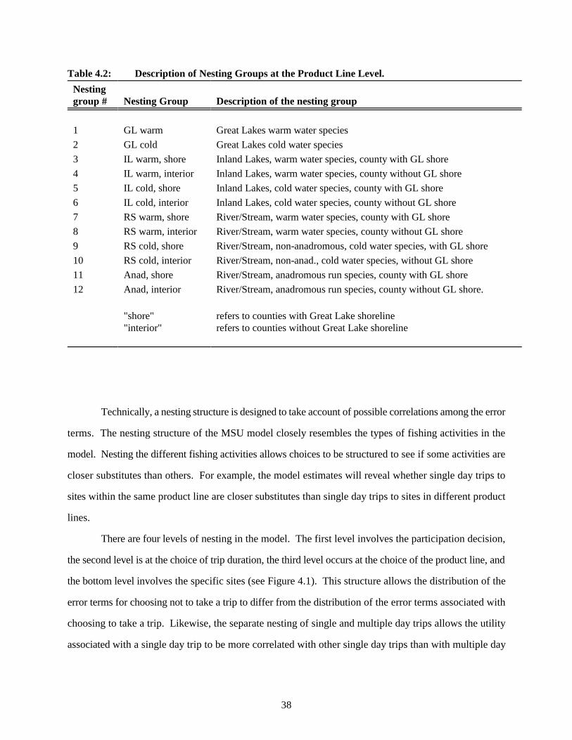
38
Nestinggroup # Nesting Group Description of the nesting group
1 GL warm Great Lakes warm water species
2 GL cold Great Lakes cold water species
3 IL warm, shore Inland Lakes, warm water species, county with GL shore
4 IL warm, interior Inland Lakes, warm water species, county without GL shore
5 IL cold, shore Inland Lakes, cold water species, county with GL shore
6 IL cold, interior Inland Lakes, cold water species, county without GL shore
7 RS warm, shore River/Stream, warm water species, county with GL shore
8 RS warm, interior River/Stream, warm water species, county without GL shore
9 RS cold, shore River/Stream, non-anadromous, cold water species, with GL shore
10 RS cold, interior River/Stream, non-anad., cold water species, without GL shore
11 Anad, shore River/Stream, anadromous run species, county with GL shore
12 Anad, interior River/Stream, anadromous run species, county without GL shore.
"shore""interior"
refers to counties with Great Lake shorelinerefers to counties without Great Lake shoreline
Table 4.2: Description of Nesting Groups at the Product Line Level.
Technically, a nesting structure is designed to take account of possible correlations among the error
terms. The nesting structure of the MSU model closely resembles the types of fishing activities in the
model. Nesting the different fishing activities allows choices to be structured to see if some activities are
closer substitutes than others. For example, the model estimates will reveal whether single day trips to
sites within the same product line are closer substitutes than single day trips to sites in different product
lines.
There are four levels of nesting in the model. The first level involves the participation decision,
the second level is at the choice of trip duration, the third level occurs at the choice of the product line, and
the bottom level involves the specific sites (see Figure 4.1). This structure allows the distribution of the
error terms for choosing not to take a trip to differ from the distribution of the error terms associated with
choosing to take a trip. Likewise, the separate nesting of single and multiple day trips allows the utility
associated with a single day trip to be more correlated with other single day trips than with multiple day

Here the Jones and Sung nesting structure has been extended for non-Great Lakes product lines to32
distinguish between counties that do and do not have Great Lakes shoreline. The rationale is that suchdestinations allow of wider portfolio of fishing types on any given trip; e.g., one can fish on a Great Lake andalso an inland lake. This is a particularly important effect for multiple day trips.
39
trips. In addition, the nesting at the product line level allows utilities for sites within a product line to be
more correlated with the utilities for sites in the same PL than for sites in different PL's.
One note on the nesting at the product line level is in order. Recall from the above discussion that
there are seven basic product lines. In the nesting structure used in the MSU model, the inland lakes,
rivers and streams, and anadromous run categories have been further subdivided to distinguish whether
the site is in a county that has Great Lakes shoreline. Unlike the product line designation, the shoreline32
distinction is mutually exclusive; a county is either in the group of counties that contain Great Lake
shoreline or it is not. The nesting at the PL level simply subdivides the existing PLs. As a result, within
each trip length there are a total of twelve nested groups corresponding to shoreline and product line
combinations. The twelve combinations are defined in Table 4.2 and are illustrated in Figure 4.1.
Bear in mind that the nesting structure is simply a way of grouping alternatives that are likely to
be similar to one another. Whether the alternatives are similar or not is revealed during the model
estimation. The four levels of nesting in the MSU model add parameters to the model estimation. These
are the parameters on the inclusive value indices which were introduced in Chapter 3. If these parameters
are significantly less than one, then the nesting structure does capture some underlying similarities among
sites within a nest. If the parameters on the inclusive value indices are not significantly different from one,
then the model collapses to a unnested logit or a multinomial logit.
4.2 Variables
At each level of the nested model, there are variables that serve to “explain” fishing choices. In
this section, the variables and their measurement are briefly described. A more detailed explanation of
how each variable is constructed is contained in Appendix 1, Sections 4 and 6.
4.2.1 Site level variables
The variables which are used to describe the elementary site alternatives include a price variable,
and various site quality variables.
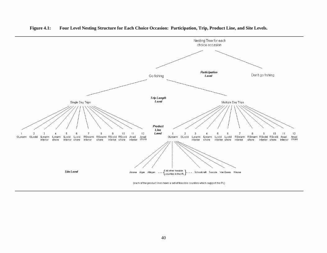
40
Figure 4.1: Four Level Nesting Structure for Each Choice Occasion: Participation, Trip, Product Line, and Site Levels.

41
Trip price: The trip price in the MSU model is the travel cost variable. Travel costs are specified
as the sum of driving, lodging, and time costs. Driving costs are the product of the individual's per mile
driving cost and the number of round trip miles from an individual's city of origin to the site. For this
study, per mile driving costs were specified as the predicted fuel cost per mile plus 14.1 cents per mile for
depreciation (American Automobile Association). The predicted fuel cost was obtained from a regression
using self-reported fuel costs. The variables used in this regression were: distance traveled on the trip, and
dummy variables for whether expenses were shared, whether a boat was towed, and whether a truck was
used. The regression was used to predict fuel costs for each individual based on each individual's usual
travel behavior. Thus, the predicted per mile driving costs were individual-specific with an average value
of 25 cents per mile. For more detail, see Appendix 1, Section 6.4.
Lodging costs were also individual-specific. From the survey data, the average per-night cost was
calculated for the following categories of lodging: hotel, camping, cabin, and other. Each individual was
also asked about their usual lodging type for overnight trips. Each individual was then assigned the sample
average lodging cost that was associated with their usual lodging type. The per night costs were then
multiplied by 3 to reflect the cost of lodging for a multi-day trip. There are no lodging costs for single day
trips.
Finally, the time cost component of the trip price was the predicted value of an individual's time
multiplied by the length of time required for a particular trip duration. The predicted value of an
individual's time came from a regression of wages on demographic variables. Single day trips were
assumed to require 8 hours of time and multi-day trips required 3.5 days of eight hours each, or 28 hours
of time. Complete details of the wage equation are provided in Appendix 1, Section 6.6.
Catch Rates (CR): Catch rates for various species in the GL warm, GL cold, and Anad product
lines are included in the model. In the GL warm product line, catch rates were computed for yellow
perch, walleye, northern pike, bass (which includes smallmouth bass, largemouth bass, bluegill, and
pumpkin), and carp (which includes carp, freshwater drum, catfish, and suckers). In the GL cold line,
catch rates are included for chinook salmon, coho salmon, lake trout, and rainbow trout. For the Anad
product line, catch rates are included for chinook salmon, coho salmon, and rainbow trout. These catch
rates were computed from MDNR Creel Survey data and were employed by Jones and Sung.
Specifically, catch rate equations were estimated by specie for sites with creel data, and this equation was
These were Poisson regressions for count data, implemented by Douglas Jester of the MDNR.33
42
used to predict catch rates at all sites. Predicted catch rates vary monthly throughout the open-water33
season. Section 4.2.1 of Appendix 1 provides additional information as well a summary statistics for the
catch rates by species and by month.
Inland lakes: In the IL warm product line, the total surface area (in acres) of warm water inland
lakes within the county is included in the model. Similarly, for the IL cold product line, the total surface
area (in acres) of cold water lakes within the county is included. Two-story lakes are contained in the
total lake acreages for both product lines.
Quality of streams: In both the RS cold and RS warm product lines, the miles of stream in various
quality categories in the county are included. The categories are top quality main stem, secondary quality
main stem, top quality tributary, and secondary quality tributary. These categories were determined by
the MDNR. The MDNR has measured the miles of warm stream and cold steam in each category for
each county in Michigan. In the MSU model, the main stem and tributary miles were combined. These
stream quality variables reflect the overall ability of the stream to produce a high-quality fishery for
desirable game fish. The inland lake and stream variables are discussed in more detail in Appendix 1,
Section 4.2.2 -- see also the tables accompanying that section.
Cabin: This dummy variable was used to identify whether an individual had a cabin, cottage, or
vacation home in a particular county. The cabin information was collected in the survey. The effect of
this variable was allowed to differ by trip duration but it does not differ across product lines within a
given trip length.
4.2.2 Other levels of nesting
Constants: When possible, choices (or branches of the nesting structure) were distinguished by
including constants. Recall from the discussion of the nesting structure that there are 24 distinct groups
at the product line level of the nesting structure -- 12 combinations of product lines and Great Lake/non-
Great Lake counties, and 2 trip lengths. There are 22 dummy variables distinguishing the various
combinations of product lines and Great Lake/non-Great Lake counties -- eleven each in the single and
This is a necessary condition for global consistency; see McFadden (1981) or Morey. A local condition34
can be derived which allows the coefficient on the inclusive value to be larger than one, but this does not givemuch leeway beyond the global condition in our model (Herriges and Kling).
43
multiple day branches of the model. There is also a constant at the trip duration level and another
constant at the participation level. In logit type models, constants assure that the estimated model fits the
observed sample data at the level of the constant. That is, where a constant appears in the model, the
baseline model predictions at the level of that constant will match the sample predictions. For example,
since the MSU model contains a constant at the participation level, the model's baseline predicted trips
will match the number of trips in the sample data. The baseline model predictions are the predictions that
result from evaluating the model at same data values that were used during estimation.
Demographics: At the participation level of the model, demographic variables are included to
distinguish among different types of anglers. The demographic variables include sex, age, and years of
education.
At the trip duration level, the model includes a variable that allows individuals who were
employed to have a different value of time than those who did not have a paying job. The variable serves
as a shifter for the predicted value of time for individuals without a paying job. The variable was created
by interacting an employment dummy with each individual's predicted wage. Specifically, the dummy
variable took the value 1 if the person did not have a paying job and zero otherwise, and this dummy was
multiplied by the person’s predicted wage. The parameter for the resulting shifter variable is only
identified at the trip duration level of the model.
Inclusive values: As described earlier, at each level of the decision tree, an inclusive value index
is included from the next lower level of the nesting structure. Since the MSU model has four levels, there
are three inclusive value indices -- at the participation level, at the trip duration level, and at the product
line level (see Figure 4.1). The inclusive value index is not a separate variable. Rather, the inclusive
value index is used to identify parameters of the statistical distribution of nested logit models. If the
parameter on the inclusive value is significantly less than 1, then the nested logit is preferred to a simple
multinomial logit. In order for the model to be consistent with the economic theory outlined above, the
estimated coefficients on the inclusive value indices need to lie between zero and one.34
The sequential estimates are consistent, but not efficient. The sequential t statistics are inflated because35
the standard errors do not account for the fact that the inclusive value is itself a random variable.
44
4.2.3 Estimation
The model was estimated in two stages. The lower three levels of nesting (trip length, product
line, and site) were estimated at one time, using full information maximum likelihood methods (FIML).
In the second stage, the participation model is estimated. The second stage employs a sequential
estimation method for nested logits, using the inclusive value estimate from the lower three levels as one
of the explanatory variables. A FIML routine that would have permitted the model to be estimated in35
one stage was explored. However, the sequential strategy allowed more cases to be included in the
analysis because a case that did not have complete details of the location of a fishing trip could be used
at the participation level of the model even though the information would not be suitable for use at the
site choice levels of the model; in the four-level FIML such a case would need to be dropped because the
joint probability of the event could not be computed. Moreover, it took approximately one month for the
FIML estimation of the first stage of the model, the lower three levels, on a Pentium personal computer.
Thus, due to the size of the estimation problem and the less stringent data requirements, the above two
stage approach was adopted.
4.3 The Survey Data
In order to estimate the parameters of the MSU model, the data describing the sites and types of
trips was combined with behavioral data about angler's fishing trips. The behavioral data revealed what
individuals chose to do on each choice occasion. The behavioral data used in the model came from a
survey of Michigan residents who were identified as potential anglers. These data included demographic
information about individuals, where they went fishing, how often they went fishing, along with details
of their fishing trips. This section provides an overview and summary of the survey. A more complete
discussion is provided in Appendix 2.
4.3.1 Survey overview
The survey was used to learn about the locations of individuals' fishing trips. An important goal
of the survey was to obtain accurate data on the number and types of trips individual anglers take in

The MDNR has experimented with alternative mail survey formats. A comparison of three month and36
annual recall periods demonstrated that frequent anglers' recall of trips is substantially biased upward with thelonger recall period (Jester, personal correspondence).
45
Michigan over the course of a fishing season. Since it is difficult to remember the details of what one
does over the course of a season, especially if there are many events to recall, the survey developed for
this project followed a sample of anglers throughout the 1994 fishing season. This type of study is called
a panel survey. Recall difficulties have been shown to increase with the length of the recall period and
the number of intervening fishing events (WESTAT). A panel study where individuals are followed36
over time can mitigate recall problems. In the MSU panel survey, the length of time between individual's
panel interviews was varied depending on the anticipated frequency of an individual's fishing activities.
In this way, recall periods were shorter for anglers who fished often.
There are three main types of interview methods for conducting survey research: in-person
interviews, telephone interviews, and mail surveys. Given the goals of the study, a telephone format was
selected as the best mode of survey administration. Telephone surveys allow for both flexibility and
control over how data is collected. In particular, the telephone method facilitates control over who
answers questions, how questions are presented, and the order in which information is presented. In a
telephone interview, questions can be used to screen and categorize respondents so that they are only
asked relevant questions. For example, one question can be used to determine whether or not a panel
member has fished since the last contact. In-person interviews are impractical in this regard, and response
rates in a mail survey might suffer from the necessity for repeated mail-backs.
The telephone survey was implemented using a Computer Assisted Telephone Interviewing
(CATI) system. One advantage of CATI surveys is that the survey instrument can be programmed to
utilize complex skip patterns without having to depend on the interviewer or the respondent to follow the
appropriate skip patterns. A CATI instrument can also be programmed so that questions automatically
utilize information that was provided in response to previous questions and earlier interviews. For
example, when asking panel members whether they fished since the last interview, the CATI system
provided the date of their last interview along with the date and location of their last trip. Tailoring the
survey instrument to each individual can improve the accuracy of respondents' answers, reduce the length
of the interview, and reduce the cognitive burden of the interview on respondents. The CATI system also

46
made it easy to track the status of each case. For example, the system tracks the time and disposition of
all call attempts on a particular case.
All of the project's telephone interviewing was conducted by the Survey Research Division (SRD)
of the Institute for Public Policy and Social Research (IPPSR) at Michigan State University. SRD uses
a CATI system which is operated over a local area network. SRD's CATI system also includes a
sophisticated phone call scheduler that automates the process of scheduling callback interviews.
There were many steps involved in the development of the full survey instrument. The process
began with a review of other related travel cost surveys. Before drafting any survey instruments,
qualitative research was conducted via four focus groups composed of Lansing-area anglers. A great deal
of use was made of a pilot survey, including feedback from interviewers, reading of case notes, and
analysis of the pilot data. Researchers also listened to mock interviews, conducted pretest calls,
monitored interviews, and debriefed interviewers. In addition, comments were sought and received from
a team of external peer reviewers. A complete discussion of these steps is contained in Appendix 2.
The survey research contained two stages: a pilot survey and the full survey. The pilot survey was
a small-scale version of the full survey. The pilot survey was conducted during the fishing season of
1993, and the full survey was conducted in 1994. The pilot survey allowed the MSU team to thoroughly
pretest and develop the survey questions. The pilot also provided an opportunity to determine some of
the parameters of the population. The knowledge acquired from the pilot survey enabled the design of
the full survey to be optimized.
Both the pilot and the full surveys consisted of two phases: a screening interview to recruit
potential anglers into the panel and the subsequent panel interviews. The samples were based on
stratified, randomly selected telephone numbers of Michigan residents. The number of panel interviews
for panel participants depended on their reported frequency of angling. Each time panel participants were
called, they were asked about their fishing activities since the previous interview.
4.3.2 The survey sample
The telephone sample was drawn from the phone numbers for the general population of Michigan
residents. A list of randomly generated numbers was purchased from Survey Sampling, Inc. (SSI) in
Fairfield, CT. The system SSI uses to generate the numbers is discussed in Appendix 2. To improve the

That fact that males in Michigan fish more than females is based on the pilot information, license sales37
data, and previous surveys (Mahoney et al).
47
efficiency of the screening interviews, the sample of telephone numbers was stratified. The stratification
was done by county, so that the proportion of numbers from each county matched the proportion of
licensed anglers in that county. There were 13,561 telephone numbers from which an attempt was made
to obtain an interview.
The initial telephone contact was a screening interview to identify potential anglers and recruit
them into the panel. An adult (age 18 or older) respondent was selected from the household. Because
males are more likely to fish than females , males were over-sampled in the screening interviews. In37
households with both male and female adults, a male was chosen two-thirds of the time while a female
was chosen one-third of the time. In households with multiple male or female adults, a random adult
member of the household was recruited by asking for the individual that most recently celebrated a
birthday.
When the data are analyzed and the welfare estimates are extrapolated to the population, this
differential sampling pattern must be accounted for. To do this, weights were created to appropriately
adjust for the stratification based on county population of licensed anglers, the male-female ratio, the
number of adults in the household, and the number of telephone lines. The exact procedure for
calculating these sample weights is described in Appendix 2, Section 5.3.2.
6,342 individuals completed the screening interview. A response rate can be calculated in various
manners, depending on what factors are taken as the “appropriate” denominator. The response rate for
completing the screening interviews is between 62% and 75% depending upon the method of calculating
response rates. Section 4 of Appendix 2 presents the disposition codes for the survey so that any desired
method of calculating response rate can be applied to the data.
After correcting for the sample stratification scheme used in the screening, there was evidence
that persons responding to the screening interview were slightly different than the Michigan population
as a whole. To correct for these differences, case weights were created for each sampled person. These
case weights were calculated so that the screening sample matched regional census data regarding the age
distribution, distribution of educational attainment, and ratio of males to females. This was done for each
of three regions of the state defined for this study: the three-county Detroit metropolitan area, lower
48
Michigan (the lower portion of the lower peninsula), and upper Michigan (the northern lower peninsula
and the upper peninsula). These regions are depicted in Figure A1.2 of Appendix 1. For complete details
of the weighting, see Section 5 of Appendix 1.
The screening interview was a short interview that asked a few questions about fishing and a few
demographic questions (see Appendix 2, Section 6 for the text of this instrument). The screening
interviews for the full survey were conducted from late March through early May, 1994. Anyone who
indicated that they fished in the previous year and/or that they were “likely” to fish during the upcoming
year was asked to participate in the panel study. Thus, the population of interest was Michigan residents
who are “potential anglers,” where potential is measured by either having fished in the previous year or
having stated an intention to fish in the upcoming season. All others are considered to be non-anglers.
The project did not consider the impact that changes in fishing quality might have on movements between
the potential and non-angler groups. For example, cleaning up a contaminated site may benefit anglers,
and may entice some individuals who do not now fish to take up the sport. This latter effect was not
included in the analyses, and, to the extent that it occurs, the MSU approach leads to an underestimate
of the benefits of the clean-up.
Of the 6,342 individuals who completed the screening, 3,415 respondents were potential anglers,
and were recruited to the panel. Of these, 2,668, or 78%, agreed to participate in the panel. Of those that
agreed to participate in the panel, 2,135, or 80%, completed all waves of the panel. In the analysis, only
data for individuals who completed the panel was used.
4.3.3 The design of the survey
Each time a set of panel interviews was conducted they were referred to as a wave. Basically,
the panel wave interviews consisted of asking whether respondent fished or not, and if they fished they
were asked a set of questions about each trip. A general outline of the survey instrument is found in
Figure 4.2.
The CATI instrument employed a rostered structure that could accommodate complex trip types.
The roster system consists of a programming loop and flexible data storage method for questions which
get repeated a different number of times for different respondents. The MSU instrument had two levels

49
of rostering. First, there was a loop through a set of questions about each trip. Second, within each trip
there was a loop through a set of questions about each site.
The final panel wave also included a number of general questions about the respondents' fishing
preferences, usual practices, boat and cabin ownership, and job characteristics. Respondents were also
asked about their chances of fishing during the winter. Those respondents who indicated they were likely
to fish during the winter were contacted once more in a wave of interviews that asked about any winter
and/or ice fishing they may have done.
The timing of panel waves was designed so that the more frequent anglers were called more often
than the infrequent anglers. Using the responses to screening questions, panel members were partitioned
into three groups based on their anticipated frequency of fishing. The group of frequent anglers was
called six times in the period from April through November. The middle range group was called four
times while the group of infrequent anglers was called twice. The grouping of respondents and the
number of waves for each group was based on an analysis of the pilot data. The goal was to obtain the
highest quality data on as many trips as possible keeping budget constraints in mind. The scheduling of
the panel waves balances the cost of the panel against the desire to reduce the recall period since the last
interview. Another factor that was taken into account was feedback from the pilot survey indicating that
infrequent anglers did not want to be called frequently, even if the interview was short. Some detailed
information such as the trip length or date was obtained on about 85% of the trips taken by the survey
sample.
Each time panel members were called they were asked how many times, if any, they had fished
since their last interview. To avoid double counting of trips and to help respondents answer the question,
interviewers would remind respondents of the date of their last interview along with the date and location
of the last trip they took. This technique is referred to as bounded recall.
The survey instrument was structured to loop through a set of questions for each time an
individual said they fished since their last interview. Inevitably, there were some individuals who could
not or would not provide the details of some of the trips that they reported they had taken. To
accommodate these individuals, there was an escape key built into the program. The escape key permitted
an interviewer to leave the loop of trip questions prior to completing all of the questions within the loop
for each trip. If this option was exercised, the respondent was given an opportunity to revise the total

50
GENERAL OUTLINE OF A PANEL WAVE INTERVIEW
1. Ask if R fished, and if so how many times R fished
2. Trip Loop (for each time R fished) ���������<
Month and Date of trip Was it an overnight trip? Number of sites fished at
Site Loop (for each site on this trip) ��� <
Name and location of site Time spent fishing at site Species tried to catch at site Was a boat used?
Repeat Site Loop for each site on this trip ��
Main site (if multiple site trip) Purpose of trip Lodging question (if overnight trip) Transportation questions (first trip only)
Repeat Trip Loop for each trip for this wave ������
3. Some Final Closing Questions
Figure 4.2: Structure of Panel Interview.
number of trips that they previously said they had taken. This was done by reminding the respondent of
how many times they said they fished and how many of these times they reported on. They were then
asked if they wanted to change their answer about the number of times they fished since their last
interview. These revisions were included to minimize any recall bias in the trip count information.
Because there are thousands of places to go fishing in Michigan, it was not possible to have
closed response categories for the locations where anglers went fishing. That meant that each time an
angler was asked where they went fishing, the interviewers would have to type in open ended text
describing the name and location of each site. However, most anglers only fish at a handful of sites. In
the pilot, 91% of the people who fished did so at three or fewer different sites. Because of this, in the first
wave interviews, some of the panel members were asked about up to three sites where they usually fish.

51
These sites were then saved for each individual and subsequently used as individual-specific closed
response categories in the site location portions of the first interview and all ensuing interviews. For trips
to one of the usual sites, the interview was shorter because interviewers were able to avoid asking and
typing text for the full set of questions about a site's name and location. Panel members in the infrequent
angler group were not asked about their usual sites since they don't fish much.
To streamline interviews, interviewers did not ask the full set of site and trip questions for repeat
visits to the same site. Within any interview, if an angler took more than two single day trips to one of
their usual sites, the angler was asked if it was a typical trip to that site. If so, the interview would move
on to the questions about the next trip.
In the screening process, some of the respondents who agreed to be in the panel were asked if
they would like to receive a fishing log. The logs provided a place to record most of the information
interviewers asked about in the panel interviews. The logs served as memory aids with the potential for
speeding up the interviews. Again, since infrequent anglers do not fish much, they were not asked if they
wanted a log. During the panel interviews, respondents with logs were asked if they wanted to use their
log while completing an interview. If they used the log, their interview was more direct. If they did not
want to read all the information from the log over the phone, interviewers offered to send them a
replacement log along with a postage paid return envelope for the original log.
Appendix 2 contains a complete discussion of all the survey efforts and presents summary results
from the survey.
4.3.4 The analysis sample
The analysis sample, upon which the model was estimated, consisted of a subset of the survey
respondents and the trips they reported. There are two sets of criteria for determining what data gets used
to estimate the model. The first set of criteria specify which of the survey respondents are eligible for
inclusion in the model estimation. Eligible respondents are basically respondents who have complete
panel data. The second set of criteria specify which trips were eligible for use in the model estimation.
Eligible trips are trips by eligible respondents where all the necessary details of the trip are known. The
analysis sample is described in detail in Appendix 1, Section 4.1.
An eligible respondent is a case which satisfies the following five conditions:

52
(1) the respondents completed the panel, and
(2) the month of every trip the respondent took is known, and
(3) there are valid observations for the respondent's demographic variables, and
(4) there are valid observations for the cabin questions, and
(5) the case was not flagged for errors (see Appendix 1, Section 4.1 for details).
If a case did not satisfy the conditions for complete panel data, then that respondent (case) is not included
in the analysis. There were 1,902 people that met the above criteria. All of these cases were used in the
participation level of the model, and all of their valid trips were used in the trip levels of the model (see
conditions below).
It is possible that implementing these exclusions might result in a sample that is not representative
of the overall population of potential anglers. Therefore, a set of weights were created for the analytical
sample that matched it to the (weighted) sample that was recruited to the panel, i.e., the "potential" anglers
identified in the screening interview. This weighting process assured that the distribution of
characteristics of anglers in the analytical sample matched the distribution of angler characteristics in the
original sample of recruited anglers. The characteristics matched by this process include the angler's
avidity group, the region of the state the angler lived in, the anglers age, and some additional demographic
variables. Details are provided in Appendix 1, Section 5.
Recall that the model is estimated in two stages: first, the trip stage estimates the trip, product
line, and site levels of the model; second, the participation stage estimates the participation level of the
model. All of the above data were needed for a person to be included in the estimation of the
participation stage of the model. These individuals can be referred to as valid individuals for purposes
of the estimation of the trip stage of the model. Additional data was needed for a trip to be used in the
trip stage of the estimation. Valid observations for the trip stage are those trips by valid individuals which
satisfy the following criteria:
(1) the destination county is known, and
(2) the product line is known, and
(3) the trip duration (single or multiple day) is known, and
(4) the trip occurred between April 1, 1994 and October 31, 1994, and
(5) the purpose of the trip was fishing, and
The “true” � coefficient is not identified in this model. The coefficients are identified up to a scale38
parameter. This does not matter for welfare measurement, where the scale parameters cancel out. At theproduct line level, the relative scale parameters differ for single and multiple day trips. Thus, to compare thesite level coefficients across day and multiple-day trips, the coefficients should be multiplied by thecorresponding coefficient on the inclusive value in the PL choice parameter estimates.
53
(6) the product line is feasible for the county visited, and
(7) the trip has not been flagged for errors, and
(8) the trip distance is less than 150 miles for day trips.
Recall that the choice occasions are 3.5 days in length, and that only one trip could be taken per choice
occasion. A small number of respondents had more trips in some month than there were choice occasions
for that month. In such cases, a random integer was assigned to each of the individual's valid trips for
the month, and the following additional selection criterion was imposed:
(9) the trip's random integer does not exceed the number of choice occasions in that month.
4.4 Estimation Results
This section reports the results of the model estimation. Recall the structure of nesting in the
MSU model: at the topmost level is a decision about participation on a choice occasion, at the next level
is choice of day or multiple-day trip, then there is the choice of product line, and finally there is the choice
of site. Recall too that the model was estimated in two steps. First, the site choice, product line choice,
and duration choice components were estimated jointly in a single “trip choice” model. The trip choice
portion of the model seeks to explain the nature of a trip if one was taken, and this part of the model was
estimated using full information maximum likelihood techniques. Then, the participation model was
estimated, using the inclusive value index from the trip choice model as a variable explaining whether
people go fishing at all on a given choice occasion. The parameter estimates are presented in two tables
corresponding to the two stages of model estimation.
In each of the tables, the column labeled “Coefficient” gives the estimate of the parameter
associated with the variable named in the first column. These are estimates of the � parameters discussed
in general terms in Section 3 of this report. The column labeled “t-statistic” gives the result of a38
statistical test of whether the coefficient is significantly different from zero (significance in the statistical

This is an asymptotic t-value on a two-tailed test of the null hypothesis that the coefficient is equal to39
zero. This is a test of a population mean of a normally distributed variable with unknown variance. It isasymptotic in that the parameter estimates will be exactly normally distributed only as the sample size becomesinfinitely large, but the approximation is good in large samples.
The significance level gives the probability of erroneously deciding the parameter is not zero, when in40
fact it is. The 20% significance level falls at t equals 1.28, 10% at t equals 1.65, 5% at t equals 1.96, and 1%at t equals 2.58.
A coefficient lying between zero and one is a sufficient condition for a well-behaved density; see41
footnote 8 above.
54
sense, not an “importance” sense). This measures the contribution of that single variable taken alone39
to the overall explanatory power of the model. The larger the number, the more highly statistically
significant the associated coefficient estimate. Speaking generally, a t-statistic greater than 2 indicates
significance.40
Table 4.3 presents the estimated parameters associated with variables in the trip duration, product
line and site choice portions of the model. These parameters were estimated simultaneously in the first
stage of the model estimation. Whenever possible, parameters were allowed to differ for single and
multiple day trips. Thus, in Table 4.3 there are two sets of columns representing the estimated coefficient
and t-statistic for single-day and multiple-day trips. The rows represent the variables which are grouped
according to their role in the model.
The first set of rows in Table 4.3 reports the values of parameters from the trip duration level of
the model, i.e., the choice between single day and multiple day trips. The three trip duration variables
are the inclusive value parameter, a constant, and a time value shifter. For convenience, these three
variables are presented in the single day column of Table 4.3, even though there is no distinction between
parameters for single and multiple day trips at this level of the model. The parameter on the trip level
inclusive value index determines the importance of the nesting structure at this level. The coefficient is
in a range that is consistent with theory. Since the coefficient is significantly less than one, separating41
the two trip lengths into different nests was an improvement over not making the distinction. That is, the
unmeasured characteristics of a trip of a particular duration are more correlated with those of a trip of the
same duration than with a trip of a different duration.
In addition to the inclusive value parameter, there is a trip duration constant which distinguishes
single from multiple day trips. The trip duration constant takes a value of zero for single day trips and
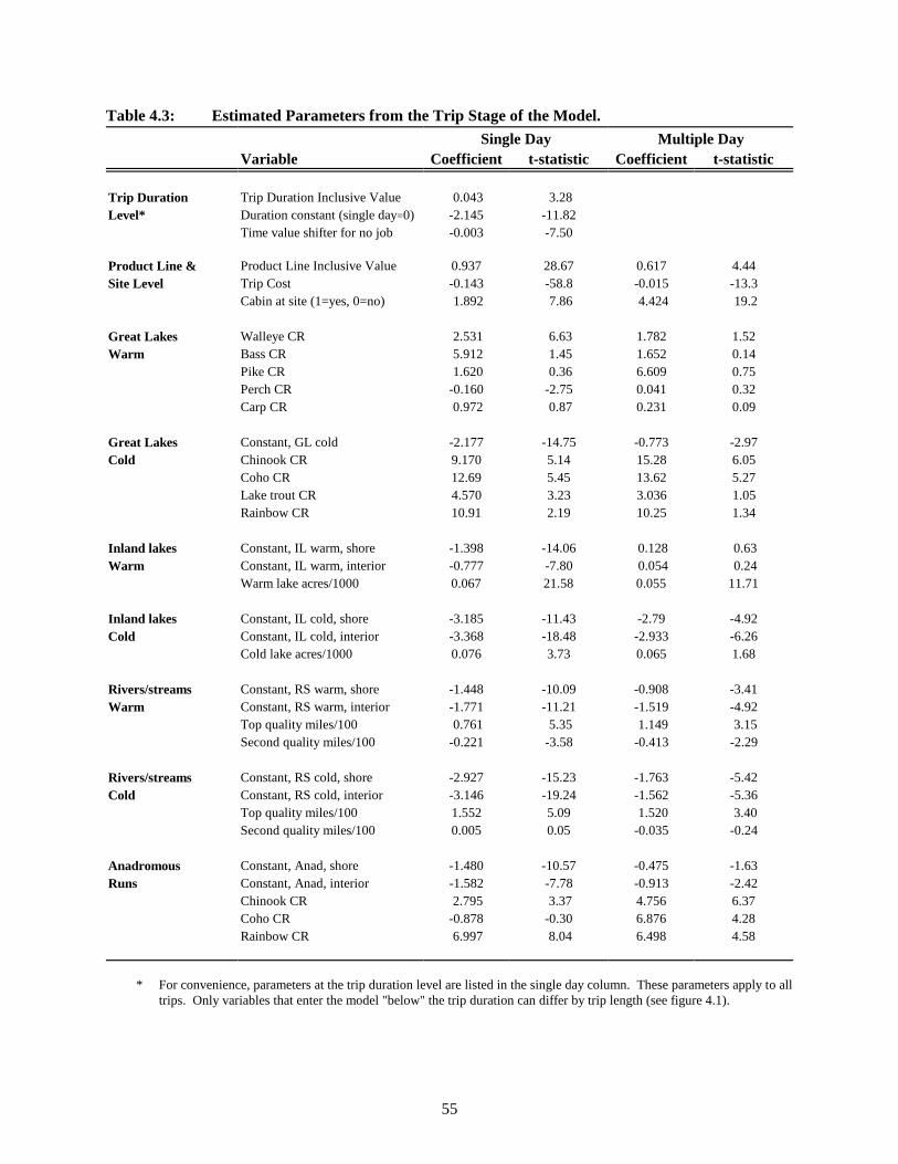
55
Single Day Multiple DayVariable Coefficient t-statistic Coefficient t-statistic
Trip Duration Trip Duration Inclusive Value 0.043 3.28Level* Duration constant (single day=0) -2.145 -11.82
Time value shifter for no job -0.003 -7.50
Product Line & Product Line Inclusive Value 0.937 28.67 0.617 4.44Site Level Trip Cost -0.143 -58.8 -0.015 -13.3
Cabin at site (1=yes, 0=no) 1.892 7.86 4.424 19.2
Great Lakes Walleye CR 2.531 6.63 1.782 1.52Warm Bass CR 5.912 1.45 1.652 0.14
Pike CR 1.620 0.36 6.609 0.75Perch CR -0.160 -2.75 0.041 0.32Carp CR 0.972 0.87 0.231 0.09
Great Lakes Constant, GL cold -2.177 -14.75 -0.773 -2.97Cold Chinook CR 9.170 5.14 15.28 6.05
Coho CR 12.69 5.45 13.62 5.27Lake trout CR 4.570 3.23 3.036 1.05Rainbow CR 10.91 2.19 10.25 1.34
Inland lakes Constant, IL warm, shore -1.398 -14.06 0.128 0.63Warm Constant, IL warm, interior -0.777 -7.80 0.054 0.24
Warm lake acres/1000 0.067 21.58 0.055 11.71
Inland lakes Constant, IL cold, shore -3.185 -11.43 -2.79 -4.92Cold Constant, IL cold, interior -3.368 -18.48 -2.933 -6.26
Cold lake acres/1000 0.076 3.73 0.065 1.68
Rivers/streams Constant, RS warm, shore -1.448 -10.09 -0.908 -3.41Warm Constant, RS warm, interior -1.771 -11.21 -1.519 -4.92
Top quality miles/100 0.761 5.35 1.149 3.15Second quality miles/100 -0.221 -3.58 -0.413 -2.29
Rivers/streams Constant, RS cold, shore -2.927 -15.23 -1.763 -5.42Cold Constant, RS cold, interior -3.146 -19.24 -1.562 -5.36
Top quality miles/100 1.552 5.09 1.520 3.40Second quality miles/100 0.005 0.05 -0.035 -0.24
Anadromous Constant, Anad, shore -1.480 -10.57 -0.475 -1.63Runs Constant, Anad, interior -1.582 -7.78 -0.913 -2.42
Chinook CR 2.795 3.37 4.756 6.37Coho CR -0.878 -0.30 6.876 4.28Rainbow CR 6.997 8.04 6.498 4.58
* For convenience, parameters at the trip duration level are listed in the single day column. These parameters apply to alltrips. Only variables that enter the model "below" the trip duration can differ by trip length (see figure 4.1).
Table 4.3: Estimated Parameters from the Trip Stage of the Model.

56
a value of one for multiple day trips. The estimated parameter for the trip duration constant shows that
people are less likely to take multiple-day trips. Finally, at the trip duration level there is a variable that
alters the value of time for individuals with jobs relative to those without jobs (see Section 2 of Appendix
1). That the estimated coefficient is negative suggests that those without jobs have a higher cost of using
their time to go fishing than those who have a job. In effect, individuals without jobs are less likely to
take multiple day trips.
After the trip duration choice, the next set of variables in Table 4.3 represent variables at the
product line level and site level. The first of these is the inclusive value index for the product line level
nesting. The coefficient on the product line inclusive value is positive and between zero and one, as it
should be (see previous footnote). Each of the combinations of product lines and Great Lake/non-Great
Lake counties has a nest specific constant term. While these are identified at the product line level of the
model, in Table 4.3 they are grouped within each of the PLs. Along with the explanatory variables within
each PL, these constants serve to fit the model with the sample shares corresponding to each PL.
The next two rows of Table 4.3 present two site level variables which share the same parameter
across all product lines: trip cost and cabin. If a person has a cabin at a site it is more likely they will
visit that site, with the influence greater on multiple-day trips. Both the single and multiple day cabin
variables are highly significant. For both day and multiple day trips, the travel cost variable is negative
(as expected) and significantly different than zero. This shows that the farther away a site is (all else
constant), the less likely it is that it will be visited. This effect is larger in the day trip branch than the
multi-day branch, indicating that for single day trips, the cost of travel is (relatively) more important.
These variables were initially constrained to be the same across trip durations, but that specification was
rejected by a likelihood ratio test. The implication is that the marginal utility of income differs by trip
length, an issue which is discussed further when model is used for policy evaluations.
In the Great Lakes warm product line, the estimated parameters are for catch rates for the
individual species. Taken as a group, these catch rates are statistically significant contributors to the
model for day trips. That is, if all of these catch rates are removed from the model, the model does a
significantly poorer job of explaining fishing behavior. Catch rates are not significant at typically-
employed significance levels for multiple day trips for warm water Great Lakes trips. The coefficients
on the catch rates for the single day model tell us that higher bass and walleye catch rates are highly

57
sought after (all else constant), while northern pike, carp and yellow perch catch rates are less sought
after. The negative sign on yellow perch catch rates is unexpected; one might guess a priori that yellow
perch would have a positive influence, larger than carp. This kind of result might arise because catch
rates for perch are correlated with other factors that influence choice. For example, sites with high yellow
perch catch rates might be composed primarily of smaller fish, whereas sites with lower catch rates might
have a greater share of larger more desirable fish.
In the Great Lakes cold product line, the estimated parameters are for catch rates for the individual
species. The catch rates for each specie have a positive influence on both single and multiple day trips.
Within the single day trips, all of the species significantly contribute to the model's explanatory power.
For multiple day trips, the salmon catch rates are significant, yet the trout catch rates are not. Taken as
a group, the multiple day trip parameters on catch rates are significant. For both the single and multiple
day trips, chinook salmon, coho salmon, and rainbow trout are relatively more desirable than lake trout.
For the inland lakes warm water product line, the inland lake acres is a highly significant variable.
The estimates indicate that all else equal, a county with more acres of warm water inland lakes is more
likely to be the destination of single and multiple day trips. Similarly, in the inland lakes cold product
line, acres of cold water lakes has a positive effect on the chance of a county being selected for either trip
length. The parameter on cold lake acres in the IL cold PL is significant at any standard significance level
for single day trips. However, for multiple day trips in the IL cold PL, the parameter on lake acres is only
significant at the 10% level.
For the river and streams warm product line, the variables for the miles of top quality and the
miles of second quality stream are both significant for single and for multiple day trips. Top quality
stream miles positively influence site choice, while second quality stream miles negatively influence site
choice. For the RS cold product line, top quality stream miles again have a significant and positive
influence on site choice for both the single and multiple day trips. Second quality stream miles are not
significant for either the single or multiple day trips portions of the RS cold product line. For the
anadromous run product line most of the catch rate variables are significant and positive for single and
multiple day trips. However, the coho catch rate for single day trips is negative, though it is not a
significant variable.
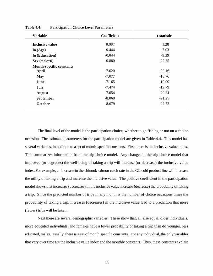
58
Variable Coefficient t-statistic
Inclusive value 0.087 1.28
ln (Age) -0.444 -7.03
ln (Education) -0.844 -9.29
Sex (male=0) -0.880 -22.35
Month-specific constants April -7.620 -20.16
May -7.077 -18.76
June -7.165 -19.00
July -7.474 -19.79
August -7.654 -20.24
September -8.068 -21.25
October -8.679
-22.72
Table 4.4: Participation Choice Level Parameters
The final level of the model is the participation choice, whether to go fishing or not on a choice
occasion. The estimated parameters for the participation model are given in Table 4.4. This model has
several variables, in addition to a set of month-specific constants. First, there is the inclusive value index.
This summarizes information from the trip choice model. Any changes in the trip choice model that
improves (or degrades) the well-being of taking a trip will increase (or decrease) the inclusive value
index. For example, an increase in the chinook salmon catch rate in the GL cold product line will increase
the utility of taking a trip and increase the inclusive value. The positive coefficient in the participation
model shows that increases (decreases) in the inclusive value increase (decrease) the probability of taking
a trip. Since the predicted number of trips in any month is the number of choice occasions times the
probability of taking a trip, increases (decreases) in the inclusive value lead to a prediction that more
(fewer) trips will be taken.
Next there are several demographic variables. These show that, all else equal, older individuals,
more educated individuals, and females have a lower probability of taking a trip than do younger, less
educated, males. Finally, there is a set of month specific constants. For any individual, the only variables
that vary over time are the inclusive value index and the monthly constants. Thus, these constants explain

59
monthly variation in fishing trips that is not accounted for by the changes in the inclusive value index.
They indicate that, all else equal, fishing trips are more likely to occur in May than in October.
4.5 Model Predictions Using the Baseline Data
This section explains how the estimated recreational demand model can be used to predict the
demand for fishing trips in Michigan. This section also presents the results of using the model to predict
trips for the baseline site data with which the model was estimated. As discussed above, the MSU model
relates fishing trips to variables describing the characteristics of fishing sites. The model is then capable
of producing estimates of changes in demand for fishing as site characteristics change. In this sense, the
model can be used to directly evaluate policies which affect site characteristics that are in the model.
Predictions of changes in trips can be made for each type of fishing trip and site that is in the model.
Chapter 5 illustrates how the model can be used to evaluate policies which affect site characteristics.
4.5.1 Procedure for predicting trips
Before using the model to produce statewide estimates of fishing in Michigan, it is important to
bear in mind that the estimates are based on the model. As such, the estimates only apply to the type of
fishing activities included in the model. For example, the estimates do not include fishing by non-
residents as only Michigan residents are included in the sample. Likewise, the estimates do not include
fishing trips with primary purposes other than fishing since these trips were not included in the model.
Here, a brief explanation of how the estimated model is used to predict statewide trips is provided.
First, for each individual in the estimation sample, individual data and the site data are combined with the
estimated parameters to compute each individual's probability of visiting each site on each choice
occasion. Summing these site probabilities up across the choice occasions in the season gives that
individual's predicted demand for trips to each site, i.e., the predicted share of their predicted trips
associated with each site within each product line. Next, the weighted average of these seasonal shares
is calculated across individuals. The weights used at this stage are the weights that were constructed so
that the estimation sample is representative of the state population of potential anglers. The result of this
stage gives the site demands for a representative potential angler in Michigan. It remains to extrapolate
these to the state by multiplying by the estimated population of potential anglers in Michigan. The
60
population of potential anglers was estimated from the screening sample, and it too was weighted so that
it would be representative of the state population of potential anglers. For complete details of the
extrapolation procedure see Section 2.4 of Appendix 1.
The results are statewide predictions of trips to each site within each product line. These can be
added up within a product line and a trip length to produce aggregate estimates of trips within each
product line. Likewise, the aggregate number of single and multiple day trips is derived by summing
across the single and multiple day product lines.
The above method of estimating trips in the baseline is different than simply extrapolating from
the sample, a process often referred to as calculating the sample shares. The difference stems from the
use of the model to predict each individual's actions. In the sample a person either does or does not visit
a site during a choice occasion. In contrast, the model predictions are probabilities of visiting a site. For
this reason, the trip predictions based on actual visited sites (sample shares) can differ from the model
predictions. These differences will depend on the extent to which the model fits the underlying data.
With the MSU model specification, the model predictions for the sample will match the corresponding
sample shares at the participation, trip length, and product line levels. This result is due to the presence
of the constant terms at the participation, trip length, and product line levels of the model. This property
does not hold for the individual sites in the model since the model does not contain site-specific constants
at the site level. Site level constants would add about 850 additional parameters to the model estimation
(one for each site within each PL and trip duration).
4.5.2 Statewide predictions of trips
The model predicts that during the open water season there were about seven million single day
trips and 1.3 million multiple day trips in Michigan made by Michigan residents for the primary purpose
of fishing. The predicted distribution of these trips across product lines is presented in Table 4.5. Bear
in mind that these are not exact numbers, rather they are estimates based on the model predictions.
The final columns of Table 4.5 provide an estimate of total recreational fishing user days by
product line. A rough calculation of user days was made by multiplying the multiple day trips times 3.85
and adding them to the single day trips. Recall that 2.85 was the average nights away for the sample. This
method of calculation yields an estimate of 12 million user days for fishing in Michigan by state residents.
Of the 12 million estimated user days, 58% are due to single day trips.

61
Product Line
Single Day Trips by PL
Multiple DayTrips by PL
Total UserDays by PL†
GL warm 2,082,100 29% 180,200 14% 2,776,100 23%
GL cold 299,900 4% 161,700 12% 922,400 8%
IL warm 3,091,500 44% 628,900 48% 5,512,900 46%
IL cold 113,000 2% 22,000 2% 197,600 2%
RS warm 971,600 14% 124,600 10% 1,451,500 12%
RS cold 225,000 3% 94,200 7% 587,900 5%
Anad 278,500����
4% 99,800����
8% 662,600����
5%
Totals* 7,061,600 1,311,500 12,110,800
† User days are defined by multiplying multiple day trips by 3.85 and adding single day trips.
* All numbers rounded to nearest one hundred. Totals may not add up due to rounding.
Table 4.5: Statewide Estimates of Fishing Trips and User Days in Michigan During the Aprilto October Season.
Figure 4.3: Trips and User Days byType of Water Body.
Figures 4.3 and 4.4 depict the total estimated
single day trips, multiple day trips, and user days. Figure
4.3 also shows the proportion of total estimated single
day trips, multiple day trips, and user days at sites with a
water body type that is a Great Lake, inland lake, or a
river/stream. Inland lakes are predicted to receive more
trips than any other water body type. The model predicts
that inland lakes are the main site for 46% and 50% of
single day and multiple day trips, respectively.
Excluding anadromous fishing, 33% (26%) of single (multiple) day trips are to Great Lakes sites. Rivers
and streams, including anadromous runs, are predicted to receive 21% (25%) of single (multiple) day trips.
These results can be derived from Table 4.5.

62
Figure 4.4: Trips and User Days byTarget Species Type.
Figure 4.5: Michigan Population,Percent per County.
Figure 4.4 shows the proportion of total
estimated single day trips, multiple day trips, and user
days that are attributable to trips targeting warm water
and cold water species. The vast majority of the
estimated trips target warm water species. The model
predictions indicate that about 87% of day trips are
within warm water product lines, while 71% of multiple
day trips are in warm water product lines. About 80% of
the estimated user days are attributable to trips targeting
warm water species. These results can be derived from Table 4.5.
4.5.3 Single day trips
This section summarizes the model predictions
for single day trips by counties, while the next section
does so for multiple day trips. Complete predictions for
each of the counties for each combination of product
line and trip length are provided at the end of this
chapter. To inform the discussion of the model
predictions, the section begins with a discussion of the
distribution of the state population.
Figures 4.5 through 4.7 depict maps of the
counties in Michigan. The counties are identified in
Figure A1.1 in Appendix 1 -- see also Figure 5.6 inside
the back cover of this report. Figure 4.5 presents the
distribution of Michigan's population. The numbers represent the percentage of the Michigan population
in each county. The percentages are rounded so that counties without numbers represent counties with less
than 0.5% of the state population. Figure 4.5 makes it evident that the vast majority of the state's
population is located in the bottom half of the Lower Peninsula with a substantial concentration
surrounding the city of Detroit.

63
Figure 4.6: Distribution of PredictedSingle Day Trips.
Figure 4.6 depicts the distribution of predicted
single day trips in Michigan. The numbers represent
each county's share (percentage) of the total predicted
single day trips. The percentages are rounded so that
counties without numbers represent counties predicted to
receive less than 0.5% of the total predicted single day
trips (less than 35,000 single day trips). There are 36
counties that are predicted to receive less than 0.5% of
the single day trips. There are 31 counties that are
predicted to receive between 0.5% and 1.5% of the
predicted single day trips, i.e., between 35,000 and
106,000 single day trips. Most of these counties are
located in the lower portion of the Lower Peninsula. However, five counties that are predicted to receive
about 1% of the single day trips are located in the Upper Peninsula. Comparing these counties with the
population map illustrates the tendency of Upper Peninsula residents to take proportionally more single
day trips than do mid-Michigan and Metro area residents.
There are 16 counties that are predicted to receive more than 1.5% of the total predicted single
day trips. Nine of these fall in the 2% range, three of them are in the 3% range, and four get more than
3.5%. Not surprisingly, these 16 counties are close to or the same as the major population centers of the
state (compare Figures 4.6 and 4.5).
The model predicts that Wayne County receives the most single day fishing trips (about 1.2
million or about 16% of the total predicted single day trips). The city of Detroit, along with numerous
suburban cities, is located in Wayne which contains 23% of the state's population. Wayne County borders
the Detroit River and includes access to some of the Detroit River island recreation sites such as Belle
Isle and Grosse Ile. In addition, a portion of northern Wayne County borders and permits access to Lake
St. Clair while a portion of southern Wayne County provides access to Lake Erie. Recall that the Detroit
river and Lake St. Clair are included in the definition of Great Lake water bodies. The distribution of the
Wayne County trips across PL's follows: 65% for GL warm, 4% for GL cold, 11% for IL warm, 0% for

For counties not mentioned above, predicted single day trips are about 245,000 for Washtenaw; 205,00042
for St. Clair; 165,000 for Livingston; 150,000 for Genesee, and 110,000 for Lapeer.
64
IL cold, 13% for RS warm, 2% for RS cold, and 5% for Anad. Complete details are provided in Table
4.6 at end of the chapter.
The Metro area county of Oakland is estimated to generate the second largest share of single day
trips (about 700,000 trips or 10% of the total predicted single day trips). The vast majority of these single
day trips are predicted to be for IL warm fishing (91%). Oakland County does not support any Great
Lake fishing opportunities.
The county of Macomb, also a Metro area county, is estimated to generate the third largest share
of single day trips (about 450,000 trips or 6% of the total predicted single day trips). Macomb County
borders Lake St. Clair, and about 73% of the predicted trips to Macomb County are for GL warm fishing.
The county of Monroe, on the southern border of Wayne County, is estimated to generate the fourth
largest share of single day trips (about 300,000 trips or 4% of the total predicted single day trips).
Monroe County borders Lake Erie and about 70% of it's predicted trips are for GL warm fishing.
To illustrate the importance of the state's population centers in the predicted allocation of single
day trips, consider the three Detroit Metro counties of Macomb, Oakland, and Wayne. These counties
contain 43% of the population of Michigan, and they are predicted to receive 33% of the single day trips.
They are the top three counties in terms of the predicted shares of single day trips. Taking the importance
of the population centers one step further, consider the group of counties adjacent to and including the
three Detroit Metro counties. This group contains nine counties: Genesee, Lapeer, Livingston, Macomb,
Monroe, Oakland, St. Clair, Washtenaw, and Wayne. These counties contain 56% of the state's
population and they are predicted to receive about 50% of the all single day trips (about 3.5 million).42
Each of these nine counties is predicted to receive more than 100,000 trips, and all but Lapeer are
predicted to receive more than 150,000 trips. In fact, all but Lapeer are in the top nine counties in terms
of the predicted number of single day trips.
The other county in the top nine for predicted number of single day trips is Kent. Kent County,
which contains the city of Grand Rapids, is the fourth most populous county in Michigan with 5% of the
states adult population. Kent is estimated to generate the sixth largest share of single day trips (about
240,000 trips).

65
Figure 4.7: Distribution of PredictedMultiple Day Trips.
4.5.4 Multiple day trips
Figure 4.7 presents a map of the counties in
Michigan and the predicted distribution of multiple
day trips. Table 4.7 contains the complete predictions
of multiple day trips for each county and product line.
The numbers in Figure 4.7 represent each county's
share (percentage) of the total predicted multiple day
trips. The percentages are rounded so that counties
without numbers represent counties predicted to
receive less than 0.5% of the total predicted multiple
day trips (less than 6,600 multiple day trips). In stark
contrast to the distribution of single day trips, there
are only seven counties that are predicted to receive
less than 0.5% of the multiple day trips. All but one of these counties are located in the north west of the
Upper Peninsula.
There are 50 counties that are predicted to receive between 0.5% and 1.5% of the predicted
multiple day trips, which is between 6,600 and 19,700 multiple day trips. There are 21 counties that are
predicted to receive between 1.5% and 2.5% of the predicted multiple day trips, i.e., between 19,700 and
33,000 multiple day trips. All of these counties are located in the Lower Peninsula, and most contain
some shoreline of the Great Lakes.
Cheboygan County is predicted to receive the most multiple day trips of any of the counties in
Michigan (about 58,000). 75% of the multiple day trips for Cheboygan County are predicted to be in the
IL warm product line, and Cheboygan County is the top county for IL warm trips. Cheboygan County
contains three of the states largest inland lakes, Burt, Mullet, and Black lakes.
The next most popular counties for multiple day trips are Wayne and Mason. Wayne and Mason
Counties are each predicted to receive about 38,500 multiple day trips. Wayne County contains the city
of Detroit. Mason County is located on the Lake Michigan shoreline. About 42% of the multiple day
trips to Mason County are for the GL cold product line, and Mason is the top county for multiple day trips
in the GL cold PL.
66
Roscommon County is ranked fourth with about 37,000 predicted multiple day trips. About
34,000 of these trips are for the IL warm product line, making Roscommon the number two destination
for multiple day trips in the IL warm product line (second to Cheboygan). Roscommon contains the two
of the State's largest inland lakes, Houghton lake (the largest) and Higgins lake. The other counties
predicted to receive more than 30,000 multiple day trips are Allegan, St. Clair, Oakland, and Muskegon.
Keweenaw County is on the other end of the spectrum of trips and population. Keweenaw is a
small county located in the Upper peninsula on a remote peninsula on Lake Superior. Keweenaw County
contains less than 0.02% of the adult population of the state. As one might expect, the model predicts
that Keweenaw County receives the fewest trips for both the single day and multiple day trip categories.
Keweenaw is predicted to receive 0.05% and 0.14% of the statewide single and multiple day trips,
respectively.
4.5.5 County level predictions
In the following tables, the MSU model's predicted trips for each trip length, for each county, and
for each product line are presented. Table 4.6 presents the predictions for single day trips, while Table
4.7 presents the predictions for multiple day trips. The seasonal trips are for the months of April through
October and were derived by summing the predicted trips to site j in month m across the months.

67
Table 4.6: Predicted demand for single day trips by county and by PL for April through October.
Co# County Name GL warm GL cold IL warm IL cold RS warm RS cold Anad Total
1 Alcona 9197 2132 3109 233 1272 445 1016 17404
2 Alger 3430 2280 2205 180 787 416 484 9782
3 Allegan 48563 24137 33729 3315 20175 5965 9999 145883
4 Alpena 12397 3171 7140 516 4494 813 1424 29955
5 Antrim 16652 2750 18632 3582 2809 920 2040 47385
6 Arenac 11125 1720 4519 0 4852 1206 2310 25732
7 Baraga 4450 2919 1697 159 981 2054 581 12841
8 Barry 0 0 79332 2922 10987 3027 0 96268
9 Bay 69283 8099 17531 0 22607 0 8107 125627
10 Benzie 4682 2029 5733 783 1846 837 1325 17235
11 Berrien 38633 19613 15228 1976 13780 2877 5997 98104
12 Branch 0 0 29746 1435 8159 1712 0 41052
13 Calhoun 0 0 45022 2279 18235 4605 0 70141
14 Cass 0 0 39063 1579 5884 1896 0 48422
15 Charlevoix 5666 1530 8262 1652 1728 646 1364 20848
16 Cheboygan 3683 537 26371 1973 951 649 3654 37818
17 Chippewa 19278 3531 9273 766 4871 1629 3256 42604
18 Clare 0 0 16874 942 4544 2072 0 24432
19 Clinton 0 0 46615 3385 20110 0 0 70110
20 Crawford 0 0 8400 553 2777 2454 0 14184
21 Delta 21081 2520 5691 673 4175 3184 3202 40526
22 Dickinson 0 0 6916 372 3051 1460 0 11799
23 Eaton 0 0 48878 3588 21505 0 10637 84608
24 Emmet 2258 767 2596 244 1406 531 1427 9229
25 Genesee 0 0 118322 0 25763 8374 0 152459
26 Gladwin 0 0 17918 1035 5681 1701 0 26335
27 Gogebic 2488 1100 3646 139 793 2635 253 11054
28 GrandTraverse 19086 3969 14185 1251 4358 1359 2437 46645
29 Gratiot 0 0 26619 0 8452 2407 0 37478
30 Hillsdale 0 0 24668 1476 6138 1963 0 34245
31 Houghton 13999 5011 11793 577 3318 5349 2600 42647
32 Huron 9122 2128 4399 0 3626 0 7044 26319
33 Ingham 0 0 75730 0 26728 0 16353 118811
34 Ionia 0 0 36500 2407 17940 3721 7072 67640
35 Iosco 9017 1901 4685 418 2615 722 2325 21683
36 Iron 0 0 20847 319 1987 4703 0 27856
37 Isabella 0 0 24585 1849 6646 2431 0 35511
38 Jackson 0 0 110581 4232 25935 6455 0 147203
39 Kalamazoo 0 0 73806 3300 14107 3282 0 94495
40 Kalkaska 0 0 10351 630 2688 1448 0 15117
41 Kent 0 0 160704 6462 34212 13496 26211 241085
42 Keweenaw 2006 733 532 91 452 172 0 3986
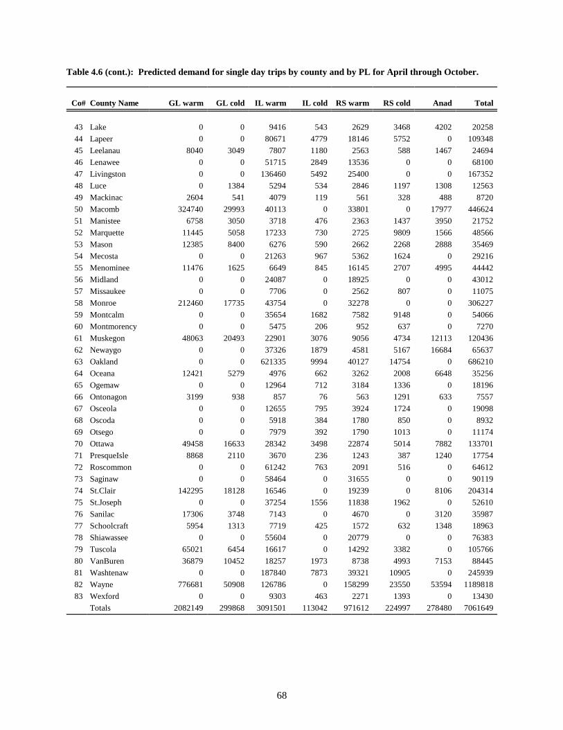
68
Table 4.6 (cont.): Predicted demand for single day trips by county and by PL for April through October.
Co# County Name GL warm GL cold IL warm IL cold RS warm RS cold Anad Total
43 Lake 0 0 9416 543 2629 3468 4202 20258
44 Lapeer 0 0 80671 4779 18146 5752 0 109348
45 Leelanau 8040 3049 7807 1180 2563 588 1467 24694
46 Lenawee 0 0 51715 2849 13536 0 0 68100
47 Livingston 0 0 136460 5492 25400 0 0 167352
48 Luce 0 1384 5294 534 2846 1197 1308 12563
49 Mackinac 2604 541 4079 119 561 328 488 8720
50 Macomb 324740 29993 40113 0 33801 0 17977 446624
51 Manistee 6758 3050 3718 476 2363 1437 3950 21752
52 Marquette 11445 5058 17233 730 2725 9809 1566 48566
53 Mason 12385 8400 6276 590 2662 2268 2888 35469
54 Mecosta 0 0 21263 967 5362 1624 0 29216
55 Menominee 11476 1625 6649 845 16145 2707 4995 44442
56 Midland 0 0 24087 0 18925 0 0 43012
57 Missaukee 0 0 7706 0 2562 807 0 11075
58 Monroe 212460 17735 43754 0 32278 0 0 306227
59 Montcalm 0 0 35654 1682 7582 9148 0 54066
60 Montmorency 0 0 5475 206 952 637 0 7270
61 Muskegon 48063 20493 22901 3076 9056 4734 12113 120436
62 Newaygo 0 0 37326 1879 4581 5167 16684 65637
63 Oakland 0 0 621335 9994 40127 14754 0 686210
64 Oceana 12421 5279 4976 662 3262 2008 6648 35256
65 Ogemaw 0 0 12964 712 3184 1336 0 18196
66 Ontonagon 3199 938 857 76 563 1291 633 7557
67 Osceola 0 0 12655 795 3924 1724 0 19098
68 Oscoda 0 0 5918 384 1780 850 0 8932
69 Otsego 0 0 7979 392 1790 1013 0 11174
70 Ottawa 49458 16633 28342 3498 22874 5014 7882 133701
71 PresqueIsle 8868 2110 3670 236 1243 387 1240 17754
72 Roscommon 0 0 61242 763 2091 516 0 64612
73 Saginaw 0 0 58464 0 31655 0 0 90119
74 St.Clair 142295 18128 16546 0 19239 0 8106 204314
75 St.Joseph 0 0 37254 1556 11838 1962 0 52610
76 Sanilac 17306 3748 7143 0 4670 0 3120 35987
77 Schoolcraft 5954 1313 7719 425 1572 632 1348 18963
78 Shiawassee 0 0 55604 0 20779 0 0 76383
79 Tuscola 65021 6454 16617 0 14292 3382 0 105766
80 VanBuren 36879 10452 18257 1973 8738 4993 7153 88445
81 Washtenaw 0 0 187840 7873 39321 10905 0 245939
82 Wayne 776681 50908 126786 0 158299 23550 53594 1189818
83 Wexford 0 0 9303 463 2271 1393 0 13430
Totals 2082149 299868 3091501 113042 971612 224997 278480 7061649

69
Table 4.7: Predicted demand for multi-day trips by county and by PL for April through October.
Co# County Name GL warm GL cold IL warm IL cold RS warm RS cold Anad Total
1 Alcona 4002 2629 7749 268 1623 914 1620 18805
2 Alger 1643 3091 2968 110 514 414 511 9251
3 Allegan 6061 13743 8856 386 2330 1344 1865 34585
4 Alpena 3427 3728 6403 216 2467 663 864 17768
5 Antrim 3986 2008 16079 1334 1563 833 1357 27160
6 Arenac 5673 1886 5160 0 2643 1068 1388 17818
7 Baraga 960 1644 1289 53 385 1021 379 5731
8 Barry 0 0 10681 376 952 1066 0 13075
9 Bay 7580 2072 6132 0 4459 0 1467 21710
10 Benzie 3649 6643 8349 495 1525 1136 3172 24969
11 Berrien 5214 10288 5564 306 2381 845 1416 26014
12 Branch 0 0 7700 337 1450 1110 0 10597
13 Calhoun 0 0 7505 341 2473 1779 0 12098
14 Cass 0 0 6907 261 620 832 0 8620
15 Charlevoix 3342 3004 11185 928 1293 840 1369 21961
16 Cheboygan 2859 1425 43611 1667 1214 1412 5829 58017
17 Chippewa 2952 1502 3681 137 905 500 802 10479
18 Clare 0 0 6674 321 1114 1891 0 10000
19 Clinton 0 0 5946 358 1637 0 0 7941
20 Crawford 0 0 4735 261 1022 2976 0 8994
21 Delta 2043 899 1829 91 648 723 594 6827
22 Dickinson 0 0 2016 93 691 778 0 3578
23 Eaton 0 0 5872 360 1663 0 1773 9668
24 Emmet 2692 2407 4595 192 1197 771 1638 13492
25 Genesee 0 0 8480 0 885 1418 0 10783
26 Gladwin 0 0 8402 410 1862 1899 0 12573
27 Gogebic 617 824 2277 45 364 1358 141 5626
28 GrandTraverse 4026 2374 9980 408 1661 882 1259 20590
29 Gratiot 0 0 5328 0 874 1098 0 7300
30 Hillsdale 0 0 6281 328 872 1171 0 8652
31 Houghton 769 497 1782 43 288 573 327 4279
32 Huron 5826 4572 5622 0 1689 0 4998 22707
33 Ingham 0 0 6619 0 1400 0 1966 9985
34 Ionia 0 0 6198 347 2227 1455 1797 12024
35 Iosco 5519 2770 8801 337 2637 1156 3905 25125
36 Iron 0 0 4611 82 482 2398 0 7573
37 Isabella 0 0 4851 302 586 1101 0 6840
38 Jackson 0 0 12494 448 2262 1835 0 17039
39 Kalamazoo 0 0 9197 379 1237 1047 0 11860
40 Kalkaska 0 0 4338 229 753 1402 0 6722
41 Kent 0 0 8665 325 1106 1743 2455 14294
42 Keweenaw 573 381 507 35 202 111 0 1809

70
Table 4.7 (cont.): Predicted demand for multi-day trips by county and by PL for April through October.
Co# County Name GL warm GL cold IL warm IL cold RS warm RS cold Anad Total
43 Lake 0 0 6150 302 1129 4668 8400 20649
44 Lapeer 0 0 7869 396 819 1330 0 10414
45 Leelanau 3240 4148 7526 490 1377 520 5222 22523
46 Lenawee 0 0 7477 364 1008 0 0 8849
47 Livingston 0 0 11799 435 1311 0 0 13545
48 Luce 0 2594 3639 163 1236 678 674 8984
49 Mackinac 2955 1863 9519 150 688 733 944 16852
50 Macomb 9930 2706 8098 0 2751 0 1819 25304
51 Manistee 4037 7094 5568 304 1821 1758 4342 24924
52 Marquette 1599 2451 5489 123 538 2080 472 12752
53 Mason 4728 16273 6882 287 1267 2112 6839 38388
54 Mecosta 0 0 8146 336 1499 1517 0 11498
55 Menominee 1324 583 1365 72 2634 391 702 7071
56 Midland 0 0 5289 0 4327 0 0 9616
57 Missaukee 0 0 4348 0 1027 1068 0 6443
58 Monroe 10430 2565 8347 0 2140 0 0 23482
59 Montcalm 0 0 7877 335 999 4804 0 14015
60 Montmorency 0 0 6439 230 788 1859 0 9316
61 Muskegon 5664 8863 8803 508 1565 1603 3486 30492
62 Newaygo 0 0 7752 356 536 2645 6792 18081
63 Oakland 0 0 28024 493 1162 2010 0 31689
64 Oceana 5681 7950 5135 284 1399 1621 4308 26378
65 Ogemaw 0 0 6876 324 1079 1586 0 9865
66 Ontonagon 822 545 1115 44 339 1020 570 4455
67 Osceola 0 0 5192 278 1002 1583 0 8055
68 Oscoda 0 0 4537 251 905 1468 0 7161
69 Otsego 0 0 4613 205 686 1402 0 6906
70 Ottawa 6170 7337 7560 395 2839 1114 1358 26773
71 PresqueIsle 3117 2401 6337 194 932 588 1490 15059
72 Roscommon 0 0 33769 516 1341 1088 0 36714
73 Saginaw 0 0 5792 0 2156 0 0 7948
74 St.Clair 11210 8480 7083 0 3679 0 1765 32217
75 St.Joseph 0 0 8010 311 2169 1081 0 11571
76 Sanilac 6361 5271 6466 0 1374 0 1493 20965
77 Schoolcraft 1955 1619 6632 181 793 512 1990 13682
78 Shiawassee 0 0 6128 0 1281 0 0 7409
79 Tuscola 7704 2121 7073 0 2604 1142 0 20644
80 VanBuren 5718 5472 7800 368 1533 1777 1986 24654
81 Washtenaw 0 0 11031 424 1466 1584 0 14505
82 Wayne 14188 2968 10266 0 7401 1573 2222 38618
83 Wexford 0 0 5189 230 869 1767 0 8055
Totals 180246 161691 628929 21958 124625 94245 99766 1311460

71
Chapter 5
Welfare Measurement with the MSU Model
This chapter discusses how the MSU model can be used to obtain estimates of the economic value
(willingness to pay) for a variety of changes in Michigan’s fishing resources. The general principles and
conceptual basis for the welfare measures are presented in Section 3.4. Here, specific examples are given
to demonstrate how the model can be used to evaluate policies which affect resource quality.
It is important to bear in mind that the policy evaluations are based on the model that was
estimated and discussed in Chapter 4. As such, the evaluations presented in this chapter only apply to
the type of fishing activities and the sample population included in the model. For example, the sample
data was drawn from the population of potential anglers in Michigan. As mentioned in Chapter 4,
potential anglers were defined as Michigan residents who either fished in the previous year or stated they
were somewhat unlikely or very unlikely to go fishing in the survey year. All other individuals were
defined as non-anglers. Therefore, changes in fishing quality that bring some non-anglers into the
population of potential anglers will generate benefits that are not captured by the MSU model.
The MSU model focuses on the recreational angling demand and welfare effects for Michigan
anglers. Yet, many individuals who reside outside of Michigan fish in the state. Welfare effects
generated by this population are not included in the MSU model. If the accounting stance taken in a
particular analysis is that of Michigan residents, then the relevant welfare effect from non-residents
consists of the income they create in Michigan via their expenditures in Michigan. If a change in
Michigan resource quality reduces (or increases) fishing in Michigan by non-residents, then the
subsequent expenditure effect will not be captured by the extant model. Alternatively, if the accounting
stance is a broader one, so that the well-being of non-residents is included in the assessment, then the
relevant measure should include the change in economic value (the WTP or WTA) for these non-
residents. Again, this is not captured by the MSU model.
In section 4.5.1 of the previous chapter, the procedure for predicting statewide fishing trips was
described. The same procedure is used here to predict trips following some change in fishing quality,
except of course, the new quality characteristics are used to make the calculations. A similar process is
In calculating the welfare measure, the travel cost parameter from the day trip portion of the model is43
used as an estimate of the marginal utility of a dollar. Recall from Chapter 4 that the estimated travel costparameter from the day trip branch of the model was substantially larger than the estimated travel costparameter from the multiple day trip branch. Using the day trip parameter results in smaller welfaremeasures because it involves dividing by a larger number.
72
used to estimate the statewide welfare effects of a policy scenario. For each individual in the sample, the
baseline and proposed site quality characteristics are used to calculate per choice occasion welfare
measures as discussed in section 3.4 of Chapter 3. These welfare measures are then summed across the
choice occasions for the season. The weighted average of these is calculated for the sample. The
weighted average WTP for the sample is then multiplied by the estimated population of potential anglers
to estimate statewide WTP associated with the policy scenario.43
5.1 Using the Existing Model
Since the MSU model relates fishing trips to variables describing the characteristics of fishing
sites, the model is capable of producing estimates of changes in demand for fishing as site characteristics
change. In this sense, the model can be used to directly evaluate any policies which affect site
characteristics that are in the model. Predictions of changes in trips can be made for each type of fishing
trip and site in the model. As well, the welfare effects (changes in economic value) of changes in the
characteristics of fishing sites can be estimated. This chapter illustrates how the model can be used to
evaluate policies that affect site characteristics. Further research would be required to use the model for
evaluations of policies affecting characteristics and sites not directly included in the MSU model.
Chapter 4 discussed the variables which describe the sites in the model. These variables include
catch rates for fish at Great Lakes sites, stream miles by quality class for both warm and cold streams, and
lake acreage for warm and cold lakes. Sites are defined at the county level and are differentiated by
product lines. Recall that product lines are combination of species type (warm or cold) and water body
(Great Lakes, inland lakes, and river/streams). Any combination of changes in these variables at any or
all sites in the MSU model can be analyzed with the existing model.
In order to conduct a policy analysis, a user of the MSU model would have to:
(1) determine the impact of the policy or event on the variables describing fishing quality in the MSUmodel,

73
(2) alter the data for the relevant variables for each of the applicable product lines in the county orcounties of interest, and
(3) run the computer programs for the policy evaluation portions of model.
In the following sections, the policy evaluation process is discussed for each of the water body types in
the MSU model. In addition, a few hypothetical examples are provided to illustrate the procedures.
5.1.1 Inland lakes
In the MSU model, inland lakes appear in two product lines for both day and multiple-day trips:
IL warm and IL cold, with two-story lakes being in both product lines. For policy purposes, inland lake
sites are distinguished by county and are described by the total warm (cold) lake acreage in the county.
If a policy altered the availability of a lake to fishing for an entire group of species, then the MSU model
could be used to value this change. Note that for the inland lake product lines, the model's only policy-
relevant variable is the total lake acreage per county. Thus, lake acreage must be considered only a crude
link between the MSU model and policies affecting inland lakes. For any given lake, there are many
available substitutes based solely in terms of lake acreage. However, if a lake has unique features that
make it especially attractive for fishing, the lake might have few high quality substitutes. Such features
are unlikely to be captured solely by lake acreage. Incorporating such features into the model would
improve the model's ability to evaluate inland lake policies.
Currently, the MSU model does not distinguish between lakes that support one or many species
within the warm (cold) species types. For example, if perch are eliminated from a lake, yet walleye
remain, there would be no reduction in warm water acreage. Thus, the model cannot evaluate policies
affecting the availability of only one species at lakes supporting several warm or cold water species.
The potential policy scenarios that can be evaluated for inland lakes are:
1) The elimination (or introduction) of a cold water lake,
2) The elimination (or introduction) of a warm water lake,
3) The reduction (or increase) in size of a cold water lake,
4) The reduction (or increase) in size of a warm water lake, and
5) A switch from cold water acres to warm water acres (or vice versa).

The policy involves removing 29,500 acres from the IL warm product line (19,600 for Houghton and44
9,900 for Higgins) and 9,900 acres from the IL cold product line (for Higgins).
74
To apply the above policies, the total change in warm (cold) lake acreage per county would need to be
determined and entered into the model's computer programs.
As an example of this type of policy analysis, consider a scenario in which, for some unspecified
reason, the fisheries in Houghton and Higgins lakes in Roscommon County are closed for one season.
Houghton lake is a large, shallow lake, supporting warm water fishing. It is well-known as an attractive
site for walleye, pike, bass, crappie, and perch fishing. Higgins lake is a large, deep lake. It is a two-story
lake, supporting both warm water species, as well as lake trout, brown trout, rainbow trout and salmon.
Hence, while Houghton lake appears only in the Inland lake warm product line of the model, Higgins is
in both the Inland lake warm and the Inland lake cold product lines.44
The analysis of a hypothetical closure of Higgins and Houghton lakes for one open water season
results in an estimated statewide reduction in welfare of about $582,000 dollars per year. The changes
in trips that result from the closure are presented in Table 5.1. The changes in predicted total statewide
trips for the season are presented for both day and multiple day trip lengths as well as a breakdown of
these changes by product lines. Table 5.1 also presents the percentage changes in trips (to derive the
percentage changes, compare to Table 4.5.)
Notice from Table 5.1 that total statewide day trips are actually predicted to increase while total
multiple day trips decrease, though the percentage change in total trips is extremely small. The results
imply that there is a slight substitution of day trips for multiple day trips which is not surprising given the
popularity of Roscommon County as a multiple day trip destination (see section 4.5.4).
Single day trips: As evidenced by Table 5.1, there is substantial substitution of other warm water
fishing opportunities as a result of the reductions in lake acreage at Roscommon County. For instance,
there is an estimated reduction of 48,100 IL warm day trips to Roscommon County. Since the net
reduction of day trips in the IL warm product line (21,600) was less than half the reduction at
Roscommon, most of the trips lost at Roscommon County are made to other sites in the IL warm product
line. Moreover, the remaining reduction in day trips to the IL warm PL are made up by increases in day
trips to other product lines.

These eight counties, their predicted increase in IL warm day trips, and their % increase in IL warm45
day trips, are: Clare 3,080 (18%); Gladwin 2,850 (16%); Ogemaw 2,700 (21%); Crawford 1,890 (23%);Isabella 1,260 (5%); Missaukee 1,280 (17%); Midland 1,240 (5%); and Osceola 1,050 (8%).
75
ProductLine
Change in Single Day Trips by PL
Change in Multiple Day Trips by PL
Change inTotal User
Days by PL†
total % total % total % GL warm 5,670 0.27 % 2,360 1.31 % 14,760 0.53 %
GL cold 1,030 0.34 % 2,080 1.29 % 9,030 0.98 %
IL warm -21,590 -0.70 % -9,060 -1.44 % -56,470 -1.02 %
IL cold 1,110 0.98 % 150 0.66 % 1,670 0.85 %
RS warm 9,300 0.96 % 1,700 1.36 % 15,840 1.09 %
RS cold 3,080 1.37 % 1,270 1.35 % 7,960 1.35 %
Anad 1,470����
0.53 % 1,170����
1.17 % 5,970����
0.90 %
Totals* 60 ~0 % -340 -0.03 % -1,240 -0.01 %
† User days are defined by multiplying multiple day trips by 3.85 and adding single day trips.
Table 5.1 Changes in Fishing Trips and User Days for Hypothetical Closure of Higgins andHoughton Lakes.
Figure 5.1 depicts the predicted change in day trips over the course of the season for the IL warm
product line as a result of a hypothetical reduction in lake acreage in Roscommon County. Roscommon
is represented by the asterisk. Most counties have little or no increase in IL warm day trips. For 42
counties, IL warm day trips are predicted to increase by less than 50 trips for 42 counties; these counties
are blank in Figure 5.1. For 65 counties, the predicted increase is less than 500 trips. From Figure 5.1,
shows that most of the substitution of IL warm day trips occurs at counties in the vicinity of Roscommon.
Eight counties were predicted to gain more than one thousand IL warm day trips. These eight counties45
either border or are adjacent to a county that borders Roscommon. It is noteworthy that these eight
counties have a total of 33,555 acres of warm lakes, just more than was lost in the scenario. Moreover,

76
Figure 5.1: IL warm Single Day Tripsunder Roscommon Policy.
these counties do not contain any lakes even close to the
size of Houghton or Higgins. This might suggest that
the model does a poor job of capturing the "uniqueness"
of large lakes such as Higgins and Houghton.
Interestingly, the total trips for the IL cold PL
actually increase even though there is a reduction of IL
cold lake acreage. The implication is that the
substitution of trips from IL warm into IL cold offsets
the loss of trips in IL cold. Most (about 60%) of the
increase in IL cold trips occur at the counties
immediately adjacent to Roscommon. The overall
increase in IL cold trips is small, and the percentage
increase in IL cold trips is about 1%.
Multiple day trips: Table 5.1 reveals that on net, there is a very small reduction in overall multiple
day trips statewide (330 trips or about 0.03% of multiple day trips). However, multiple day trips in the
IL warm product line are predicted to decrease by 25,500 at Roscommon County. Trips at other counties
in the IL warm PL are predicted to increase by about 16,500 so that over half the reduction in multiple
day trips to Roscommon is made up through substitution to other sites in the same PL. As with the day
trips, the model predicts that the reductions in multiple day trips to Roscommon County are largely made
up through substitution of multiple day trips to other counties and other PL's.
Figure 5.2 presents the increases in multiple day trips that are within the IL warm product line yet
occur at counties other than Roscommon as a result of the hypothetical closure of Houghton and Higgins
Lakes. The changes in trips are much more evenly distributed over substitute sites than were the changes
in single day trips within IL warm (compare to Figure 5.1). For single day trips in IL warm, the top 6
sites account for 50% of the increase in day trips at counties other than Roscommon, where as for
multiple day trips in IL warm, it takes the top 20 sites to account for 50% of the increase in multiple day
trips at sites other than Roscommon.
Prior to the policy, Roscommon was the number two destination for multiple day trips in the IL
warm product line (Cheboygan was number one and Oakland was number three). Under the policy

77
Figure 5.2: IL warm Multi-Day Tripsunder Roscommon Policy.
scenario, Oakland and Cheboygan are the top two
counties in terms of increases in predicted IL warm
multiple day trips; Oakland County is predicted to
receive 1,130 additional multiple day IL warm trips and
Cheboygan gets 610 more. All other counties in the IL
warm product line are predicted to receive less than 500
additional multiple day trips -- further evidence of how
spread out the impacts of the policy are for multiple day
trips relative to the more concentrated impacts for single
day trips.
As with single day trips, the IL cold product line
is actually predicted to have a net increase in multiple
day trips as a result of the hypothetical closure of Higgins and Houghton lakes. There is a predicted
reduction of 200 multiple day IL cold trips to Roscommon County (a 40% reduction). These losses are
more than made up by substitution to other sites in the IL cold product line. The increases in multiple day
IL cold trips are very spread out across counties in the IL cold product line. For example, the largest
increase in multiple day IL cold trips occurs at Cheboygan which is predicted to receive only 20 more trips.
5.1.2 Great Lakes and anadromous runs
In the Great Lakes product lines (warm and cold) and Anadromous run product lines, the relevant
policy variables included in the model are the catch rates for various fish species in the alternative
destination counties. This is true for both day and multiple-day trips. The catch rates vary over the
season, and they vary across counties. The catch rates are also specific to distinct species within the PL's,
i.e., they are not grouped into one catch index for each PL. Policies that alter any or all of the catch rates
for these species can be valued using the MSU model. The species are:
GL Warm: yellow perch, walleye, pike, carp, and bass.
GL Cold: coho salmon, chinook salmon, lake trout, and rainbow trout,
Anad: coho salmon, chinook salmon, and rainbow trout.

78
Figure 5.3: Lake Huron Counties.
To conduct a policy analysis using the catch rates, policy makers would need to identify: the counties
affected by the policy; the species within those counties that are affected; and the months during which
the catch rates are affected.
If a policy or event eliminates a specie of fish (or group of species) from a Great Lakes product
line, this can be evaluated by either (1) reducing the catch rate for that specie to zero, or (2) deleting that
county from the set of possible places to go in that product line if all species are eliminated for that PL.
As an example of an evaluation of a policy
scenario which affects catch rates, suppose that there is
a policy which results in a 10% increase in catch rates in
all cold water species for Lake Huron. Such a policy
would involve the counties shown in Figure 5.3. The
policy includes changes in cold specie catch rates for
Lake Huron counties in the GL cold product line, and for
the anadromous runs that occur in those counties as
shown in Figure 5.3. There are 13 counties that have
shoreline that borders Lake Huron, and of these, 12
support some anadromous runs.
Before examining the policy results, some context is in order. Under the baseline conditions, the
average Lake Huron catch rates for cold species are very low, and most are zero. Therefore, a 10% increase
in catch rates actually results in a very small absolute change in catch rates. To see why this is the case,
consider some statistics characterizing the baseline catch rates.
Since catch rates in the MSU model vary on a monthly basis, there are seven months of catch rate
values for GL cold (April through October), and there are four months of catch rate values for Anad (April,
May, September, and October). GL cold contains four distinct species and Anad contains three. In addition,
there are 13 GL cold counties and 12 Anad counties that are affected by the Lake Huron policy (see Figure
5.3). Consequently, there are 508 combinations of specie, month, and county where catch rates can change
as a result of the hypothetical 10% increase in Lake Huron cold species catch rates. However, of these 508
county/month/specie combinations, only 148 (29%) of these end up being affected by the policy because the
other 360 (71%) combinations have zero catch rates prior to the policy.
The average is calculated as the simple sum of catch rates over the feasible months (7 for GL cold46
and 4 for Anad) and feasible Lake Huron counties (13 for GL cold and 12 for Anad) divided by thenumber of month/county combinations (91 for GL cold or 48 for Anad).
79
In addition to the fact that catch rates are zero for many of the county/month/specie combinations,
the average catch rates are quite low for the Lake Huron cold species. In the GL cold product line,
average hourly catch rates for Lake Huron are 0.03 for chinook salmon, 0.02 for lake trout, and zero for
coho salmon and rainbow trout. For the Anad product line, average hourly catch rates for Lake Huron
are 0.05 for chinook salmon and rainbow trout and zero for coho salmon. Thus, the 10% increase46
results in an increase in the average Lake Huron cold specie catch rates that ranges from a low of zero
to a high of one fish per 200 hours for chinook salmon on anadromous runs.
The analysis of a hypothetical 10% increase in the Lake Huron cold water catch rates for one open
water season results in an estimated statewide increase in welfare of about $82,000 dollars per year. The
changes in trips that result from the increased catch rates are presented in Table 5.2. The changes in
predicted total statewide trips for the season are presented for both day and multiple day trip lengths as
well as a breakdown of these changes by product lines. Table 5.2 also presents the percentage changes
in trips (to derive the percentage changes, compare to Table 4.5.) The results in Table 5.2 show slight
decreases in the total predicted single day trips that are offset by slight increases in the total predicted
multiple day trips. However, these changes are negligible.
Single day trips: For single day trips, there is a predicted increase of 4,700 single day trips in the
Anad and GL cold product lines. About 260 of these come from substitution away from other sites within
these product lines, and the rest are drawn from other product lines. Half of these 260 trips are drawn
from Macomb and Wayne Counties, and about one third of them are drawn from Lake Michigan sites.
Table 5.2 reveals that most of the day trips are drawn from other product lines with a slight decline in
overall day trips. Thus, for this policy (which affects a large share of sites in the Anad and GL cold PL's),
there is little substitution away from sites within the PL's relative to substitution from other PL's.
Most of the Lake Huron policy counties experience increases in combined Anad and GL cold
multiple day trips, though Bay, Tuscola, and Arenac are predicted to receive slight loses in combined
Anad and GL cold multiple day trips. Three of the counties are predicted to gain more than 1,000

80
ProductLine
Change in Single Day Trips by PL
Change in Multiple Day Trips by PL
Change in Total User
Days by PL†
total % total % total %
GL warm -2,080 -0.10 % -650 -0.36 % -4,600 - 0.17
GL cold 2,450 0.82 % 2,160 1.34 % 10,790 1.17
IL warm -1,890 -0.06 % -2,270 -0.36 % -10,620 -0.19
IL cold -80 -0.07 % -80 -0.36 % -380 -0.19
RS warm -640 -0.07 % -450 -0.36 % -2,370 -0.16
RS cold -130 -0.06 % -330 -0.35 % -1,390 -0.24
Anad 2,250����
0.81 % 1,770����
1.77 % 9,050����
1.37
Totals* -110 ~0 % 150 0.01 % 470 ~0%
† User days are defined by multiplying multiple day trips by 3.85 and adding single day trips.
Table 5.2: Changes in Fishing Trips and User Days for Hypothetical 10% Increase in Troutand Salmon Catch Rates at all Lake Huron Sites.
multiple day trips (combining Anad and GL cold product lines); the three counties are Cheboygan
(1,500), St. Clair (1,300), Huron (1,110), with the remaining gains spread across Lake Huron counties.
For combined multiple day trips in the Anad and GL cold product lines, the reductions in trips
are more spread out across counties than they were for single day trips. For the multiple day trips, 17
counties account for 75% of the reductions in trips to the Anad and GL cold PL's, as compared with 4
sites for the single day trips. In addition, within the combined Anad and GL cold PL's, only 7% of the
reductions in trips occur at Wayne and Macomb Counties, where as these two counties accounted for half
the comparable reductions for single day trips.
Consider the affects of this policy on multiple trips in the "non-policy" PL's, i.e., in the GL warm,
IL warm, IL cold, RS warm, and RS cold. Summing the loses in multiple day trips for each county in the
non-policy PL's, the counties losing the most multiple day trips are Cheboygan (200), Roscommon (130),
Wayne (120), Macomb (120), and St. Clair (90). All other counties lose less than 90 multiple day trips

81
in total across the non-policy PL's. Again, for the non-policy PL's, the multiple day trip changes are more
spread out than they are for single day trips. The five counties losing the most multiple day trips in the
non-policy PL's (see above) lose 17% of total trips lost to these PL's, as compared to 38% for single day
trips. In addition, the metro counties accounted for 21% of the losses in non-policy PL's for single day
trips, while for multiple day trips, the metro counties only account for 9% of the losses in non-policy PL's.
This example policy allows us to highlight some of the substitution patterns that occur within the
model. Since the hypothetical increase in catch rates improves the quality of Lake Huron, one might
wonder what the impacts are on other Great Lakes sites. For single day trips, reductions in trips to Lake
Michigan are limited because Lake Michigan is not in the single day trip choice set for a large segment
of the potential angler population (Detroit residents). This means that for single day trips, there is less
possibility for substitution of sites within the affected PL's. When this effect is combined with the scale
of the policy (a large share of each persons Anad and GL cold sites are affected by policy), the model
predicts relatively more substitution across PL's for single day trips. This intuition helps to explain the
larger relative loses in the Metro counties for single day trips than for multiple day trips.
5.1.3 Rivers and streams
In the Rivers and Streams product lines (warm and cold, day and multi-day), the variables
included in the model are the miles of (warm or cold) streams in the county in two quality categories: top
quality and secondary quality. Top quality streams support good self-sustaining stocks of desirable game
fish. In secondary quality streams, game fish populations are appreciably limited by such factors as
pollution, competition, or inadequate natural production. These quality designations, assigned by the
MDNR, do not represent any broader concept of quality in terms of scenic beauty, access, etc. Additional
details on these variables are provided in Section 4.2.2 of Appendix 1.
Using this information, two types of policy scenarios could be evaluated using the MSU model.
First, a stretch of river or stream could lose and/or gain a species type. For example, a river supporting
both warm and cold water species could lose the cold water species due to some pollution event or fishery
management action. Evaluating such an impact would involve decreasing the number of miles of cold
water river in the relevant quality categories for the counties affected by the impact. Likewise, a warm
stream could have its fish no longer available and the miles of warm water river would fall. A second

82
type of policy scenario would involve a stretch of river or stream that changed quality categories, e.g.,
a change from top quality to secondary quality (or the reverse) as a result of a pollution event or fishery
management actions.
To provide an illustration of this type of analysis, consider a hypothetical policy that results in
100 miles of secondary quality warm water stream in Oakland County being improved to top quality.
Oakland County is part of the Detroit metropolitan area and is shown on the map in Figure 5.4 as
indicated by the asterisk. The increase in top quality stream miles would make Oakland one of the best
counties in the state as measured by miles of top quality warm streams per county. For the exact stream
miles in top and secondary quality in each county consult Table A1.3 in Appendix 1.
The analysis of a hypothetical change of 100 miles of Oakland County secondary quality streams
to top quality streams for one open water season results in an estimated statewide increase in welfare of
about $476,500 dollars per year. The changes in trips that result from the Oakland policy are presented
in Table 5.3. The changes in predicted total statewide trips for the season are presented for both day and
multiple day trip lengths as well as a breakdown of these changes by product lines. Table 5.3 also
presents the percentage changes in trips (to derive the percentage changes, compare to Table 4.5.)
The results in Table 5.3 imply that there are slight increases in the total predicted single day trips
that are offset by slight decreases in the total predicted multiple day trips. However, as with the other
hypothetical policies examined in this chapter, these changes are negligible.
Single day trips: As presented in Table 5.3, there is a substantial increase in RS warm single day
trips as a result of the hypothetical Oakland stream improvement. RS warm single day trips increase by
53,000 (5.5%). Almost all of this increase in trips is offset by decreases in single day trips in the other
product lines. Over half the increase in RS warm single day trips is offset by decreased trips from the IL
warm product line. The trips drawn from IL warm amount to a 1% decrease in the total single day trips
in that product line. Most of the remaining trips are drawn from the GL warm product line.
The model predicts that RS warm single day trips increase at Oakland County by 61,300. From
Table 5.3 it is clear that most of these trips are drawn from other product lines, though 8,000 trips are
drawn from other sites within the RS warm product line. Figure 5.4 depicts the changes in the pattern
of single day trips. The upper figure shows the decreases in single day trips that occur at sites other than

83
ProductLine
Change in Single Day Trips by PL
Change in Multiple Day Trips by PL
Change in Total User
Days by PL†
total % total % total %
GL warm -18,400 -0.88 % -400 -0.22 % -19,920 -0.72 %
GL cold -1560 -0.52 % -340 -0.21 % -2,850 -0.31 %
IL warm -29,800 -0.96 % -1,430 -0.23 % -35,290 -0.64 %
IL cold -580 -0.52 % -50 -0.22 % -770 -0.39 %
RS warm 53,330 5.49 % 2,310 1.85 % 62,210 4.29 %
RS cold -1,160 -0.52 % -200 -0.21 % -1,930 -0.33 %
Anad -1,310����
-0.47 % -190����
-0.19 % -2,050����
-0.31 %
Totals* 520 0.01 % -290 -0.02 % -600 ~0 %
† User days are defined by multiplying multiple day trips by 3.85 and adding single day trips.
Table 5.3: Changes in Fishing Trips and User Days for Hypothetical Change fromSecondary to Top Quality for 100 Miles of Streams in Oakland County.
Oakland within the RS warm product line. The lower figure presents the county level changes in the
combined single day trips for all product lines other than RS warm.
From the Figure 5.4, it is clear that most of the predicted increase in RS warm single day trips to
Oakland County is offset by reductions of other types of single day trips at Oakland County and the counties
immediately adjacent to Oakland. For example, for RS warm single day trips, the largest reduction in trips
is experienced by Wayne County (1,960) followed by Washtenaw (930), Genesee (880), Livingston (730),
Lapeer (670), and Macomb (560). All of these counties border Oakland, and they account for 72% of the
8,000 trips that are lost to RS warm sites other than Oakland.
For the trips that are drawn from outside the RS warm product line, Oakland County experiences the
largest losses -- 17,200 single day trips across all other product lines. Thus, of the 61,300 trip increase in
RS warm single day trips to Oakland County, 28% of them come from single day trips to other product lines
at Oakland County. In fact, almost all of these are from IL warm at Oakland since Oakland does not support
the GL or Anad product lines. Most (84%) of the other reductions in single day trips outside the RS warm

84
Figure 5.4: Single Day Trips UnderOakland Policy.
product line come from the counties adjacent to Oakland (see
the lower diagram in Figure 5.4). After
Oakland County, the largest reductions in single day trips
from outside the RS warm product line come from the
following counties: Wayne (11,980), Macomb (6,820),
Genesee (2,520), St. Clair (2,290), Monroe (2,120),
Livingston (2,120), Washtenaw (2,110), and Lapeer (1,750).
While not immediately adjacent Oakland, St. Clair and
Monroe enter the list due to large reductions in GL warm
trips.
Multiple day trips: Inspection of Table 5.3 reveals
that the Oakland policy results in an increase of 2,300
multiple day trips in the RS warm product line, an increase of
about 2%. This increase in multiple day trips is more than
offset by reductions in multiple day trips in the other product
lines. As with single day trips, most of the trips are drawn
from the IL warm and GL warm product lines. In net, there is
a slight reduction in total multiple day trips.
The model predicts that RS warm multiple day trips
increase at Oakland County by 4,000. From Table 5.3, just
over half of these trips are drawn from other product lines, and 1,700 trips are drawn from other sites within
the RS warm product line. Figure 5.5 depicts the changes in the pattern of multiple day trips. The upper
figure shows the decreases in multiple day trips that occur at sites other than Oakland within the RS warm
product line. The lower figure presents the county level changes in the combined multiple day trips for all
product lines other than RS warm.
For multiple day trips in the RS warm product lines, the five counties losing the most trips to
Oakland County are Midland (130), Calhoun (80), Saginaw (70), Jackson (70), and Ionia (70). While these
counties are in the vicinity of Oakland, they are not adjacent to it. These five counties account for only 25%
of the multiple day trips that are drawn from other RS warm counties, as contrasted with single

85
Figure 5.5: Multiple Day TripsUnder Oakland Policy.
day trips where the top five counties accounted for 65% of
the trips that were lost within the RS warm product line.
That the impacts on multiple day trips are more
spread out than for single day trips is also true for the
changes in multiple day trips outside the RS warm product
line, as seen in the lower diagram of Figure 5.5. For the trips
that are drawn from outside the RS warm product line,
Oakland County experiences the largest losses -- 180
multiple day trips across all product lines other than RS
warm. Of the 4,000 additional multiple day trips to Oakland
County for RS warm, only 5% come from other product lines
at Oakland County. The five counties that experience the
largest reductions in multiple day trips to all other product
lines besides RS warm are, after Oakland, as follows:
Cheboygan (110), Wayne (80), St. Clair (80), and
Roscommon (70). These five counties account for only 20%
of the multiple day trips that are drawn from outside the RS
warm product line, as contrasted with single day trips where
the top five counties accounted for 77% of the trips lost
outside the RS warm product line. Thus, the impacts on
multiple day trips are much more diffuse.
5.1.4 The value of Great Lakes fish
Policies or events that result in fish kills in one of the Great Lakes can be evaluated using the MSU
model. If the biomass or number of fish and their species composition is known, and the species are
among those for which catch rates are included in the model, then the value per unit of biomass (or number
of fish) can be deduced. This would be done by translating between catch rates and biomass.
For example, suppose a spill occurs, and it is determined that X pounds of trout and salmon were
killed (or Y number of fish, at an average weight of Z). Then, as a separate calculation not part of the

86
MSU model, one could determine how this would alter trout and salmon catch rates in the relevant
counties at the relevant times of the fishing season. This change in catch rates could be valued as above
in section 5.1.2. Hence, the catch rate policy evaluations have an implied value of fish, and vice versa.
The Type-A Model for the Great Lakes Environment (Type A-GLE), produced by NOAA,
provides an assessment of the biomass of various fish species killed by a release of a number of different
hazardous substances for regions of the Great lakes. The Type A-GLE model then uses generic values
derived from a number of studies and applies them to the estimated loss of biomass in a “benefits transfer.”
It would be possible to combine the biomass loss estimate from the Type A-GLE model with highly site-
specific information contained in the MSU model to provide an alternative estimate of the losses.
Derivations of the value of lost biomass are areas for future research, and detailed examples of such an
analysis are not provided in this report.
5.1.5 Resource-based compensation
Section 2.1.4 of this report explained how measures of welfare change could be defined and
measured using compensation in a unit of account other than money. This was called compensatory
resource restoration. For a limited set of possible types of resource compensation, the MSU model can
be used to determine the location and scale of compensatory resource restoration projects. The types of
projects that lend themselves to evaluation using the MSU model must involve quality variables, or other
descriptor variables included within the model. For example, suppose a pollution event reduced miles of
top quality river in a county. The MSU model could be employed to determine the increase in and mix
of inland lake acres, and/or other river miles, and/or catch rates for Great lakes species that would be
required in various locations in order to compensate anglers for the loss in river fishing. The potential for
using the MSU model in this manner raises a number of theoretical and practical issues, a full treatment
of these issues is beyond the scope of this project and report.
5.2 General Themes from Policy Scenarios
Several general conclusions can be drawn from the estimated model and the hypothetical policy
scenarios analyzed above. From the hypothetical scenarios, it is clear that the site substitution possibilities
matter. The model embodies a wide range of substitute fishing activities and sites. Examination of the

87
changes in predicted patterns of trips following each of the hypothetical policies indicates that there is a
high degree of substitution at the site level of the model. There is also some degree of substitution at the
product line level of the model. The larger the scale of the policy in terms of the number of sites affected,
the more product line substitution exhibited by the model. Substitution of sites within the single day trip
type is driven by proximity to site(s) where quality changes, where as multiple day trip substitution
patterns are much more diffuse. Conversely, the hypothetical policies showed that there is very little
substitution across trip lengths and negligible changes in overall trips. As such, total fishing trips as
predicted by the model are very inelastic with respect to changes in site quality.
In addition, there are some general policy statements which apply to valuation models such as the
MSU model that can be emphasized here. First, because of the importance of the travel cost variable and
because each angler is treated equally in the aggregation of benefits, changes in fishing quality which occur
at sites closer to population centers have larger impacts than the same changes at similar sites that are
distant from population centers. Thus, based on differences in population, increasing fishing quality at
sites near the Detroit metro area will generate more benefits than equivalent increases in quality at similar
sites in the Upper Peninsula. Second, because marginal benefits are proportional to the probability that
a site is visited, a given change in quality generates the most benefits when applied to the site with the
highest probability of being visited. Thus, small improvements at low visitation sites are less valuable than
small improvements at high visitation sites.
5.3 Further Research
Here, some possible extensions of the MSU model are discussed. It must be stressed that the
following discussion lacks a great deal of detail regarding how data might and should be collected and
analyzed. In almost all instances, implementing the following suggestions involve complicated issues of
both a theoretical and practical nature; a serious program of research should be conducted to resolve these
issues and implement these suggestions.
5.3.1 Additional variables
The previous sections identified the types of policies that could be analyzed using the MSU model
and associated data as they now stand. If the State or some other entity were to collect additional data on

88
the characteristics of fishing destinations, then the model could be re-estimated using these augmented
data, and the scope of applicability of the model in policy analysis could be expanded. Here, some
variables that it could prove useful to collect data on in the future are identified.
The MSU model explained here only included catch rate variables for the Great lake warm, Great
lakes cold, and anadromous run product lines. It might be possible to include catch rates for inland lakes
and for rivers and streams, though this was not done due to a lack of available data. There do exist some
data on inland lake and river and stream catch rates. These have been collected over the years by the
MDNR using creel surveys. As well, in 1984, the MDNR conducted an extensive survey to collect
information on fishing behavior. However, the data are incomplete and exist for relatively few sites and
years. The coverage problem could be eased by collecting new data on catch rates at a wider number of
sites. This could be done by expanded creel surveys, which would be expensive, or by self-report via a
mail survey instrument, which would be relatively inexpensive.
It should also be noted that there may be variables other than catch rates that describe fishing
quality that might be useful to include in the model. An example would be a simple index of whether a
particular specie is available at a site. Another alternative to including catch rates directly in the model
is to collect data on exogenous variables that are indicative of relative fishing quality at inland lakes and
in rivers and streams. These would be biological and physical variables that determine the capacity of a
site to produce good fishing. Examples might be littoral acres of lakes, pool-riffle ratios for streams, and
water quality measures. Another option would be to develop predictive models of fishing quality based
on sites where more comprehensive data is available. It is especially important that improved site quality
variables be assembled for inland lakes if these product lines are to be the subject of policy analyses.
Another indicator of fishing quality that might be useful would be based on perceived fishing
quality. For example, one could have fishery experts rank or rate alternative destinations as to fishing
quality. Examples of such variables, which currently exists but are not included in the model, include the
designation as a Michigan “Blue Ribbon” fishing stream by the MDNR, and inclusion in the Michigan
United Conservation Club's listing of the 50 best fishing lakes in Michigan. A related approach would be
to ask a random sample of anglers to rate or rank fishing quality at various sites.

For each choice occasion, the MSU model already contains a very large number of combinations of47
trip types and sites (855 elemental alternatives when anadromous sites are available and 767 when they arenot). The size of the model is further compounded by the repetition of this choice structure over the seasonand the time varying nature of some of the explanatory variables.
89
5.3.2 Redefining sites
Sites in the current model are defined at the county level. It would be possible to refine the spatial
resolution of the elementary sites that are available as choices in the model. For example, inland lakes
could be individually identified and/or river and stream sites could be identified as stream segments or
watersheds. More refined site definitions may improve the correspondence between likely policy scenarios
and sites in the model, and such resolution may yield statistically better parameter estimates. The main
reasons for using county level definitions for fishing destinations in the existing model are the
computational burden of increasing the number of sites and the availability of data to describe sites at47
finer levels of spatial resolution. Of course, any redefining of sites and/or changing of variables requires
re-estimation of the model.
River and streams: The county level definition of sites is largely due to the fact that the stream
quality variables (miles top/secondary quality warm/cold) were available at the county levels. Were these
variables to be recoded at some alternative level of spatial resolution (e.g., watersheds or stream segments),
then the river and stream sites could be recoded accordingly. The behavioral data is amenable to this task
as the stream/river name and nearest city collected in the survey could be used to re-assign trips to the
appropriate watershed/river segments. Moreover, it may well be possible to redefine the river and stream
sites based on watershed units that are large enough that the number of elemental river sites, and hence
the computational burden, does not change too much.
Inland lakes: It would not be possible to enter all possible inland lakes in Michigan as individual
sites in the model because there are so many inland lakes in Michigan that the model would quickly
become intractable. Moreover, most of these lakes will never be targets of major policy actions, and data
describing these sites is unlikely to be available. Alternatively, it may be possible to model the choice
among major individual lakes by entering them individually while other lakes get defined in more
aggregated units. Such modelling choices entail making complex trade-offs between desires to include
relevant substitute fishing sites, achieving a good fit between the model and the data, obtaining statistically
desirable parameter estimates, and the tractability of the resulting model.
Contingent behavior contrasts with contingent valuation studies, which in essence ask, “contingent48
on the implementation of an action which changes the resource base in the manner described, and a cost toyou of $X to pay for the action, would you vote yes or no in a referendum on the action?”
90
Great Lakes: The Great Lakes sites are defined as the stretch of Great Lake shoreline within each
county. While the definition of Great Lake sites could be revised, there is likely to be less gain than there
might be in redefining the inland lake and/or river and stream sites. Reasons for this include the fact that
most of the GL counties contain one major recreational harbor, all the counties are likely to contain some
private marina's and smaller launch areas, and there is a good fit between the existing GL catch rate data
and the county definitions.
5.3.3 Contingent behavior
The discussion in the preceding section concerned ways to expand the applicability of the MSU
model by gathering additional data on characteristics of alternative destinations for fishing trips and by
refining the definitions of sites. This section briefly discusses ways of combining the MSU model with
additional data on the choices made by anglers in response to changes the resource base. This involves
asking anglers directly about what they would do differently if a particular change in the resource base
occurred. Then, that change in behavior could be valued using the MSU model. Such an approach is
called a “contingent behavior” study. In essence these studies ask, “contingent on the resource base
changing in the manner described, how would your behavior change?” Bear in mind that any approach48
involving contingent behavior studies would require an appropriate research program to design the study
and collect the contingent behavior data.
Values per trip/user day values: As a simple example, suppose a contingent behavior survey were
to establish changes in the number of trips or user days at some site in response to some change in site
quality. The existing MSU model could be used to derive the average value per trip to a site or the
average user day value for a site. Then these additional (lost) trips or user days from the contingent
behavior survey could be assigned the average value of trips or user days to that site.
A qualitative variables approach: In a more sophisticated linkage, suppose that in a contingent
behavior survey, respondents provide their baseline number of trips and their number of trips after some
quality change. Recall that the MSU model has in it a number of site characteristic variables that serve

91
to (partially) explain choice of fishing destinations. Any relevant variables that are not measured and
included in the model are captured by the error terms. In addition to the measured site quality variables,
one can include a set of site-specific qualitative variables (also called dummy variables) for the different
sites. These pick up the average effect of unmeasured quality variables, and then the error term is an
individual-specific deviation from these average effects. A change in the parameter on a site's dummy
variable has the same effect as changing some unmeasured quality attribute of the site.
The team has termed this the qualitative variables approach. When the magnitude of a site-
specific qualitative variable changes, the overall model changes, predicting changes in visitation at all
sites, including the policy site, via the participation and trip choice models. If one has an estimate of the
new number of trips at the policy site (and, perhaps, others as well) from the contingent behavior survey,
then, one can calibrate the site-specific variable for the policy site in the MSU model until the visitation
predictions from the model match the estimates from the contingent behavior survey. The overall welfare
change is the value to anglers of the change in the qualitative variable. More details of the approach are
discussed in Lupi et al. Such an approach would require re-estimation of the MSU model with the
additional site-specific qualitative variables.
Contingent choice experiments: The MSU model uses measures of site attributes, such as catch
rates from creel surveys, top/secondary quality streams, and acres of lakes. Other variables which may
be of policy interest may not have not been measured for all sites or their current measurement may
embody some deficiency. In some cases such obstacles can be overcome by using contingent choice
experiments (CCEs). In CCEs, the analyst presents individuals hypothetical alternatives to chose among,
where the analyst controls the characteristics of the alternatives. The analyst can identify site
characteristics of interest and construct alternative hypothetical destinations by combining different
characteristics according to some statistical design. These alternatives would be presented to an
respondent, who would choose among the alternatives. This might involve, for example, several choices
among Site A, Site B, or don’t go, where the characteristics of sites A and B in the choice are varied both
across choices for one respondent and across respondents.
A choice model could then be estimated with this data in the same manner as the MSU model.
Indeed, the choice problems facing individuals in the two models are very similar, but in one case they
are facing “real” sites, and in the other they are facing “constructed” sites. The same type of welfare

92
analysis applies as well. One can use the CCE data alone, or combine them with data from observed
choices. This issue, and the relationship between the two types of data, has been studied for recreation
choices by Adamowicz et al, 1994.
5.3.4 Technical extensions of the model
Standard errors: Currently, the MSU model can produce statewide estimates of changes in trips
and welfare effects that result from some changes fishing quality. These statewide estimates are based
upon the estimated parameters of the model, and thus, are complex functions of random variables.
Therefore, the statewide estimates are themselves random variables (Adamowicz et al, 1989). It would
be useful to have some simple way of calculating the standard errors of these statewide estimates.
However, because of the non-linearity of the underlying formulas and the number of estimated
parameters, there are no readily available calculations that can be used to derive these standard errors for
the statewide estimates. However, there are simulation based methods for approximating the standard
errors of these estimates (Kling). These approaches could be explored as candidates for deriving
estimates of the standard errors of the statewide estimates produced by the MSU model. Given the size
of the MSU model's data, these simulation methods are computationally intensive and have not been
carried out, though in principle they could be used.
Panel data estimators: The MSU model is estimated using repeated observations on the fishing
choices made by survey respondents over the course of the open water fishing season. Such data contain
multiple observations for each sample member and are often referred to as panel data. In the MSU model,
the error terms in each choice occasion are assumed to be independent of each other. However, with
panel data, it is possible that the error terms for individual i are correlated across that individual's choice
occasions. For general regression models, there are established statistical methods for dealing with such
potential correlations. Accounting for potential correlations in discrete panel data (e.g., RUM models)
is more complex, particularly for models as large as the MSU model. However, extensions of the MSU
statistical model to account for the panel nature of the data may be feasible in the near future.
93
References
Adamowicz, Wiktor L., Jerald J. Fletcher, and Theodore Graham-Tomasi, "Functional Form and theStatistical Properties of Welfare Measures," American Journal of Agricultural Economics, Vol.71, No. 2:414-21, May, 1989a.
Adamowicz, Wiktor L., Theodore Graham-Tomasi, and Jerald J. Fletcher, "Inequality ConstrainedEstimation of Consumer Surplus," Canadian Journal of Agricultural Economics, Vol. 37:407-420, 1989b.
Adamowicz, Wiktor, J. Louviere, and M. Williams, "Combining Revealed and Stated Preference Methodsfor Valuing Environmental Amenities," Journal of Environmental Economics and Management,Vol. 26, No. 3:271-292, May, 1994.
Amemyia, Takeshi, "On a Two-step Estimation of a Multivariate Logit Model," Journal of Econometrics,Vol. 8:13-21, 1978.
American Automobile Association, Your Driving Costs, 1993.
Ben-Akiva, Moshe, and Steven R. Lerman, Discrete Choice Analysis: Theory and Application to TravelDemand, Cambridge: MIT Press, 1985.
Bockstael, Nancy E., and Ivar E. Strand, "The Effects of Common Sources of Regression Error onBenefit Estimates," Land Economics, Vol. 63:11-20, February, 1987.
Bockstael, Nancy E., Kenneth E. McConnell, and Ivar E. Strand, Jr., "Chapter 8 - Recreation," in:Measuring the Demand for Environmental Quality, (Braden, John B., and Charles D. Kolstad,eds.), New York : North-Holland Publishing, 227-355, 1991.
Bockstael, Nancy E., W. Michael Hanemann, and Catherine L. Kling, "Estimating the Value of WaterQuality Improvements in a Recreational Demand Framework," Water Resources Research, Vol.23 No. 5:951-960, May, 1987.
Feather, Peter, Daniel Hellerstein, and Theodore Tomasi, "A Discrete-Count Model of RecreationalDemand," Journal of Environmental Economics and Management, Vol. 29:214-227, 1995.
Freeman III, A. Myrick, The Measurement of Environmental and Resource Values: Theory and Methods,Washington, D.C.: Resources for the Future, 1993.
Graham-Tomasi, Theodore, Wiktor L. Adamowicz, and Jerald J. Fletcher, "Errors of Truncation inApproximations to Expected Consumer Surplus," Land Economics, Vol. 66 No. 1:50-55,February, 1990.

94
Greene, William H., Econometric Analysis, New York : MacMillan Publishing Co., 1993.
Greene, William H., Limdep Version 6.0 User's Manual and Reference Guide, Econometric Software,Inc., v-xxvii, 1992.
Hanemann, W. Michael, A Methodological and Empirical Study of the Recreation Benefits from WaterQuality Improvements, PhD Dissertation, Harvard University, 1978.
Hanemann, W. Michael, "Willingness to Pay and Willingness to Accept: How Much Can They Differ?,"American Economic Review, Vol. 81, no. 3:635-647, 1991.
Hanemann, W. Michael, and Richard T. Carson, Southcentral Alaska Sport Fishing Economic Study,Report to Alaska Department of Fish and Game, Jones and Stokes Associates, 1987.
Hausmann, Jerry A., Gregory K. Leonard, and Daniel McFadden, "A Utility-Consistent, CombinedDiscrete Choice and Count Data Model: Assessing Recreational Use Losses Due to NaturalResource Damage," Journal of Public Economics, Vol. 56:1-30, 1995.
Herriges, Joseph, and Catherine Kling, "Testing the Consistency of Nested Logit Models with UtilityMaximization," Economic Letters, forthcoming: 1996.
Jones, Carol Adair, and Yusen D. Sung, Valuation of Environmental Quality at Michigan RecreationalSites: Methodological Issues and Policy Applications, Final Report, EPA Contract No. CR-816247-01-2, September, 1993.
Kikuchi, Hideo, Segmenting Michigan's Sport Fishing Market: Evaluation of Two Approaches, PhDDissertation, Michigan State University, 1986.
Kling, Catherine L., "Comparing Welfare Estimates of Environmental Quality Changes from RecreationalDemand Models," Journal of Environmental Economics and Management, Vol. 15:331-40,September, 1988.
Kling, Catherine L., and Richard Sexton, "Bootstrapping in Applied Welfare Analysis," AmericanJournal of Agricultural Economics, Vol. 72:406-418, May, 1990.
Kmenta, Jan, Elements of Econometrics, New York : MacMillan Publishing Co., 1986.
Krieger, Douglas J., The Economic Value of Environmental Risk Information: Theory and Applicationto the Michigan Sport Fishery, PhD Dissertation, Michigan State University, 1994.
Lupi, Frank, Heng Z. Chen, Theodore Tomasi, and John P. Hoehn, "Site-specific Qualitative Variablesin Random Utility Travel Cost Models," Agricultural Economics Staff Paper 94-06, MichiganState University, February, 1994.
Maddala, G.S., Limited-dependent and Qualitative Variables in Econometrics, Cambridge UniversityPress, 1983.

95
Mahoney, Edward M., Douglas B. Jester, Jr., Gale C. Jamsen, "Chapter 16- Recreational Fishing inMichigan," in: Travel and Tourism in Michigan: A Statistical Profile, (Dan Spotts, eds.), Travel,Tourism, and Recreational Resource Center. Michigan State University, 307-343, 1991.
Maler, Karl-Goran, Environmental Economics: A Theoretical Inquiry, Baltimore: Johns Hopkins Pressand Resources for the Future, 1974.
McFadden, Daniel, "Conditional Logit Analysis of Qualitative Choice Behavior," in: Frontiers inEconometrics, (Zarembka, Paul, eds.), New York: Academic Press, 105-42, 1974(3).
McFadden, Daniel, "Econometric Models of Probabilistic Choice Models," in: Structural Analysis ofDiscrete Data with Applications, (Manski, Charles, and Daniel McFadden, eds.), Cambridge:MIT Press, 1981.
MDNR, 1967a, Coldwater Lakes of Michigan, Memorandum, Michigan Department of NaturalResources, August, 1967.
MDNR, 1967b, Stream Classification, Memorandum, Michigan Department of Natural Resources,October 31, 1967.
Merna, James W., James C. Schneider, Gaylord R. Alexander, Warren D. Alward, and Randy L.Eshenroder, Manual of Fisheries Survey Methods, Fisheries Management Report No. 9, FisheriesDivision, Michigan Department of Natural Resources, January 1981.
Morey, Edward R., TWO RUMs un CLOAKED: Nested-Logit Models of Site Choice and Nested-LogitModels of Participation and Site Choice, Western Regional Research Project W-133, SeventhInterim Report, June, 1994.
Morey, Edward R., Robert D. Rowe, Michael Watson, "A Repeated Nested Logit Model of AtlanticSalmon Fishing," American Journal of Agricultural Economics, Vol. 75, No. 3:578-592, August,1993.
Parsons, George R., and Mary Jo Kealy, "A Demand Theory For Number of Trips in a Random UtilityModel of Recreation," Journal of Environmental Economics and Management, Vol. 29:357-367,1995.
Phagan, Tiffany, Estimating the Opportunity Cost of Time when Labor Supply Decisions areInstitutionally Constrained, Plan B Paper for M.S. Degree, Department of AgriculturalEconomics, Michigan Stat University, 1995.
WESTAT, Inc., Investigation of Possible Recall/Reference Period Bias in National Surveys of Fishing,Hunting, and Wildlife-Associated Recreation, U.S. Department of the Interior, Washington, D.C.,1989.

96
Figure 5.6: Michigan Counties*
{Insert full size county map on last page of Volume 1}
* For a Michigan map with the county names and codes (1 to 83), see Figure A1.1 in Appendix 1.