An Econometric Analysis of Trade Creation and Trade Diversion in Mercosur: the Case of Paraguay

Victor F. Gauto Department of Applied Economics, University of Minnesota

E-mail: gauto002@umn.edu Telephone No.: +1-612-701-3988

Selected Poster prepared for presentation at the International Association of Agricultural Economists (IAAE) Triennial Conference, Foz do Iguaçu, Brazil, 18-24 August, 2012.

Copyright 2012 by Victor F. Gauto. All rights reserved. Readers may make verbatim copies of this document for non-commercial purposes by any means, provided that this copyright notice appears on all such copies.

1

An Econometric Analysis of Trade Creation and Trade Diversion in Mercosur: the Case of Paraguay

Victor Gauto

Department of Applied Economics University of Minnesota

January 2012

Abstract

This paper analyzes the effects of Mercosur on Paraguayan import flows using detailed trade values to identify patterns of trade creation and trade diversion at aggregate and disaggregate commodity levels. It is well know that the share of foreign trade with respect to GDP is larger for small countries. Consequently, the effects of a trade agreement between large and small countries are likely to be larger in small economies. I use a variant of the gravity model employing a re-parameterization of the difference-in-difference estimator to analyze import flows over time from member and non-member countries. Additionally, I explicitly include zero trade flows and implement a Heckman sample selection correction along with country fixed effects. I find the creation of Mercosur has increased average regional imports by 266% since 1995, which is evidence of trade creation. The greatest import expansions have been in Beverages and Tobacco and Animal and vegetable oils & fats. Finally, I do not find statistically significant evidence of trade diversion in any of the ten commodity categories.

1. Introduction Regional and bilateral trade agreements have proliferated around the world over the last thirty years. The World Trade Organization1 recognizes 217 trade agreements currently in force, out of which 195 have been consummated since 1990. Mercosur and NAFTA are among the older of the more recent trade agreements having been created in 1991 and 1994, respectively. A well known phenomenon in international trade is that smaller, relatively narrow-based economies, the extreme of which are island economies and city states, tend to trade a larger share of their GDP than do larger more diversified economies (Frankel, 1997). Trade agreements between a small economy and larger economies are thus likely to have a larger effect on the share of the small economies foreign trade in GDP. The net effect on small country welfare may be positive even if the agreement results in some trade diversion provided the gains from trade expansion that would not otherwise have occurred dominate the loss from diversion. Moreover, these gains or losses are likely to be far larger for a small economy. While there have been a plethora of studies investigating the effects of trade agreements, few have focused on small economies. This paper presents an analysis of the effects Mercosur has had on Paraguayan import flows. Created in 1991, Mercosur is a regional trade agreement (RTA), functioning as a customs union, in South America made up of Argentina, Brazil, Paraguay, and Uruguay. A recent study on Mercosur’s common external tariff (CET) reported member tariff rates have changed as each country has gradually converged to the common external tariff. According to this study, Argentina, Brazil, and 1 http://rtais.wto.org/UI/PublicAllRTAList.aspx

2

Uruguay have converged down to the CET and reduced average tariff rates by 50%, 33%, and 25%, respectively. On the contrary, Paraguay has converged up to the CET and increased average tariff rates by 50% (Berlinski, 2005). This finding suggests Mercosur has raised Paraguay’s barriers to international trade. Yet, hundreds of exemptions to the CET remain and negotiations on such product categories as ‘capital goods’ and ‘information and communications technology’ have continued2. Consequently, the overall impact of Mercosur on Paraguay’s import flows is the empirical question I attempt to answer. The creation of Mercosur can be considered a natural policy experiment where the underlying variation in member and non-member tariff rates can be used to identify its impact on import flows from member and non-member countries. Although I do not use the variation in the actual tariff rate, this impact is approximated using dummy variables for member and non-member countries at the time Mercosur’s key policies went into effect. I use a rich data set, spanning over forty years, made up of trade values at the commodity level. One of the main objectives of this paper will be to identify patterns of trade creation and trade diversion at aggregate and disaggregate commodity levels. Trade creation occurs when it is less costly to import a good from an RTA member in a trade agreement than to produce it domestically, while trade diversion takes place when a least cost supplier from the rest of the world is replaced by RTA member countries benefitting from tariff-free trade. That is, the RTA favors imports from given countries. Unlike similar studies relying on the gravity model of international trade, I explicitly include ‘zero trade flow’ observations in the data to account for sample selection bias. My contribution to this literature is the employment of a re-parameterization of the difference-in-difference estimator, which I use in combination with a Heckman sample selection correction as outlined in Helpman et al. (2008). Additionally, I also control for unobserved time invariant country characteristics through fixed effects. I find the creation of Mercosur has increased average regional imports by 266% since 1995. Also, I do not find statistically significant evidence of trade diversion in any of the ten commodity categories. As a result, the expansion of imports attributable to Mercosur reflects gains which could have hardly been realized otherwise. Finally, I find heterogeneity bias from time-invariant country characteristics to be slightly greater than sample selection bias. Section 2 of this paper discusses the context of the study and related literature. Section 3 discusses the underlying conceptual framework motivating the empirical strategy. In section 4 the data and methodology are reviewed and results are presented in section 5. The paper ends with a brief conclusion. 2. Context of a study of Mercosur in the Literature 2.1 Context Examining the Mercosur share of Paraguayan imports is illustrative of the history of Paraguay’s trading relationship with its Mercosur partners. Figure 1 exhibits import shares from Mercosur and

2 The Paraguayan Ministry of Finance reports extended exemptions for 1,200 capital goods and 390 information and communications technology items (http://www.hacienda.gov.py/web-hacienda/index.php?c=96&n=3335) until 2019. Some examples of exempted goods are ‘mobile cellular phones’ (HS-2006 85171100) and ‘personal computers’ (HS-2006 84715010) which have a CET of 20% and 16% respectively. On the other hand, electrical appliances are an example of durables without exemptions, which have a CET of 20%.

3

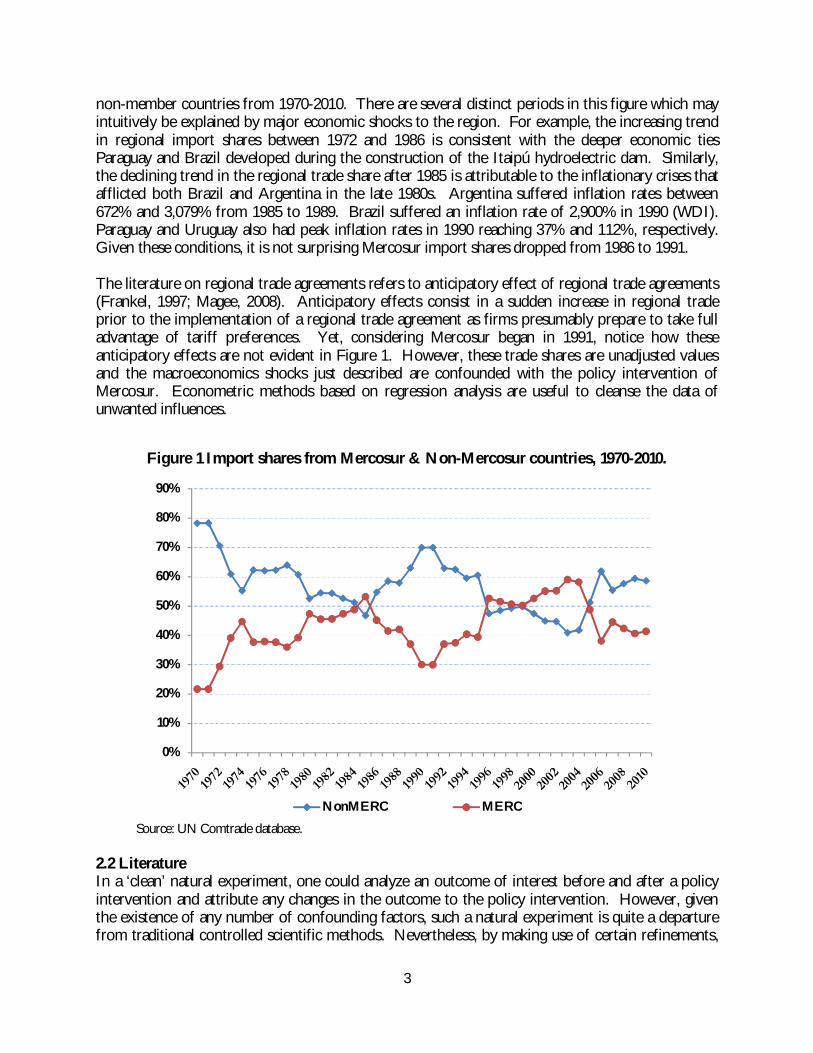
non-member countries from 1970-2010. There are several distinct periods in this figure which may intuitively be explained by major economic shocks to the region. For example, the increasing trend in regional import shares between 1972 and 1986 is consistent with the deeper economic ties Paraguay and Brazil developed during the construction of the Itaipú hydroelectric dam. Similarly, the declining trend in the regional trade share after 1985 is attributable to the inflationary crises that afflicted both Brazil and Argentina in the late 1980s. Argentina suffered inflation rates between 672% and 3,079% from 1985 to 1989. Brazil suffered an inflation rate of 2,900% in 1990 (WDI). Paraguay and Uruguay also had peak inflation rates in 1990 reaching 37% and 112%, respectively. Given these conditions, it is not surprising Mercosur import shares dropped from 1986 to 1991. The literature on regional trade agreements refers to anticipatory effect of regional trade agreements (Frankel, 1997; Magee, 2008). Anticipatory effects consist in a sudden increase in regional trade prior to the implementation of a regional trade agreement as firms presumably prepare to take full advantage of tariff preferences. Yet, considering Mercosur began in 1991, notice how these anticipatory effects are not evident in Figure 1. However, these trade shares are unadjusted values and the macroeconomics shocks just described are confounded with the policy intervention of Mercosur. Econometric methods based on regression analysis are useful to cleanse the data of unwanted influences.

Figure 1 Import shares from Mercosur & Non-Mercosur countries, 1970-2010.

Source: UN Comtrade database. 2.2 Literature In a ‘clean’ natural experiment, one could analyze an outcome of interest before and after a policy intervention and attribute any changes in the outcome to the policy intervention. However, given the existence of any number of confounding factors, such a natural experiment is quite a departure from traditional controlled scientific methods. Nevertheless, by making use of certain refinements,

0%

10%

20%

30%

40%

50%

60%

70%

80%

90%

NonMERC MERC

4

unadjusted trade shares may be cleansed of unwanted influences. In studies where a regional trade agreement is the policy intervention, confounding factors include expansions in regional trade due to anticipation by regional firms as well as macroeconomic shocks. Nevertheless, numerous studies have attempted to evaluate the impact of such policy interventions using the gravity model of international trade. These studies fall into two general categories, those simultaneously analyzing multiple trade agreements, and those analyzing the impact of single trade agreement, the former generally outnumbering the latter. The studies in the first group can be further distinguished by whether they incorporated the time dimension to the analysis. Frankel (1997), which has been the basis of this research, reported regression results of yearly cross-sections at five year intervals. He also pooled several years of data available to him and treated RTAs as fixed over time. This treatment of RTAs does not necessarily capture trade created since the policy intervention but it does give an indication of whether regional trade was disproportionately high prior to the implementation of an RTA. Similarly, Soloaga and Winters (2001) also evaluated multiple regional trade agreements in a re-parameterized gravity model. They treated zero trade flows as a data censoring problem and implemented their empirical strategy using a Tobit model. They also estimated their model on single and pooled three year cross-sectional data and studied the parameters of RTAs over time to identify any major expansions or contractions of trade flow before and after the policy intervention. These types of studies are not only used to analyze individual regional trade flows but also to address the broader question of whether RTAs are undermining the multilateral trade liberalization process3. Bayoumi & Eichengreen (1997) and Magee (2008) also analyzed multiple trade agreements simultaneously. Both incorporated interactions of RTA with time dummy variables though in Magee’s case this interaction was embedded in the model specification. Bayoumi & Eichengreen (1997) observed several European RTAs over a forty year period and found that the strongest evidence of trade creation was during the 1960s. They also found evidence of a reduction in European trade with the rest of the world. Magee (2008) accounted for zero trade flows in one of the three specifications in his study. The model accounting for the zero trade flows was estimated using a fixed effects Poisson Pseudo Maximum Likelihood estimator. Moreover, he captured yearly changes in the level of regional trade before and after the creation of RTAs by using the dummy variable interaction mentioned previously. However, including year fixed effects precluded variables capturing trade flows with non-member countries due to collinearity issues. Studies that focus on a single trade agreement using the gravity model have focused on US trading relations and the effects of NAFTA on trade flows. Clausing (2001) addressed the Canada – United States Free Trade Agreement and its effects on Canadian exports to the US. The time span of her study was from 1989 to 1994 and she used detailed tariff rates to identify the impact of the RTA on trade flows. She did not find evidence of trade diversion considering Canada’s growth in exports to the US was not at the expense of third countries that did not obtain the same preferences as Canada. Fukao, Okubo, & Stern (2003) focused on the effects of NAFTA on US imports from 1992 to 1998. Their principal specification was a panel country and year fixed effects model with a dummy variable for NAFTA countries since its creation. They did not take into account zero trade flows in their

3 Regionalism is said to undermine multilateral trade liberalization or act as a ‘stumbling block’ if RTAs hinder trade liberalization with non-member countries. Frankel (1997) finds that by his research countries entering liberal trade agreements also tend to open up with non-member trading partners, suggesting RTAs support multilateral trade liberalization or act as ‘building blocks’ for international free trade (p. 227).

5

estimation, but used a very detailed data set at the four digit level of commodity disaggregation. Additionally, rather than using trade values as the dependent variable they used shares of imports, indexed by commodity, country, and year. Similar to Magee (2008), their specification did not permit an analysis of import flows from non-member countries. They found evidence of trade diversion in the US in certain commodity categories. Finally, another group of studies analyzed changes in trade share before and after the implementation of a RTA. Krueger (1999) performed such an analysis of NAFTA while Yeats (1998) did so for Mercosur. Krueger’s (1999) study was based on a ‘shift in share’ analysis. Although she found an increase in Mexican imports, seemingly at the expense of East Asian import shares, Krueger argued that Mexican exports had gained shares in other international markets as well and therefore was not evidence of trade diversion. Yeats (1998) analyzed several trade indices from 1988 to 1994. These indices revealed that products experiencing the greatest growth in regional trade shares were not competitive in international markets. The implication being that Mercosur’s trade expansion reflected a pattern of trade diversion. One of his explanations for this finding was that Mercosur’s tariff rates were four to six times higher than those of in European RTAs. 3. Theory of Trade Creation and Trade Diversion One of the often cited gains from trade is that countries can achieve higher levels of economic welfare through trading than under autarky. Simply put, this is because countries can export goods that are more valuable in world markets abroad, and import goods which are relatively costly to produce domestically, from the rest of the world. All countries are better off in such a relationship because they achieve higher levels of consumption than would otherwise be possible. This is the argument for multilateral trade liberalization and it is also the argument that was initially used to promote preferential or regional trade liberalization. Policy-makers believed countries in regional trade agreements could obtain the gains from trade previously discussed. Viner (1950) was one of the first to argue and demonstrate that under certain conditions, regional trade agreement generated losses rather than gains. He used the example of a customs union to demonstrate how countries might actually be worse off. Viner synthesized the benefits and losses of custom unions into the concepts of trade creation and trade diversion. In the Vinerian sense, trade creation occurs when it is more efficient to import a good from a partner in a trade agreement than to produce it domestically. This is a welfare increasing consequence of an RTA because it improves the importing country’s terms of trade by expanding its consumption capacity. Trade diversion takes place when imports from efficient sources are shifted to inefficient sources that are benefitting from tariff preferences associated with membership to an RTA. This is a welfare-reducing consequence of regional trade agreements since the terms of trade of the importing country decrease by the amount of tariff revenue forgone in shifting imports to an RTA partner.

6

Figure 2

The theory of trade diversion and trade creation is based on a partial-equilibrium analysis of trade. Bhagwati and Panagariya (1996) extend Viner’s model to highlight the effects on partner countries and the rest of the world, rather than focusing exclusively on the importing country. Assume there are three countries A, B, and C. C represents the rest of the world while A and B are potential union partners. Figure 2 models import demand of a given product in country A. A’s import demand curve is represented by DD. The rest of the world’s supply (C) is assumed to be perfectly elastic and represented by the horizontal supply curve SC, while B’s supply curve is upward sloping (SB). Country B’s upward sloping supply curve will permit an analysis of welfare change in the exporting country, a feature that is absent in the original work of Viner (1950). The model below permits the analysis of various scenarios, including the gains from trade under nondiscriminatory tariffs and free trade between A and B. Subsequently, I will present the extension of this analysis for the case of Paraguay, which is a member of the customs union Mercosur. In a scenario of non-discriminatory tariffs the equilibrium price is PC+T and A imports OQ3 in total. Country B supplies OQ1, and Q1Q3 is imported from C. The gains from trade for A are given by the area under the demand curve and above the international price-line free of tariff (KHNI). This area is made up of the consumer surplus (KGI) and tariff revenue (GHNI). The gains to B are represented by the area over the supply curve SB and under the international price-line, PC, represented by triangle HWU. Suppose A enters a free trade agreement with B. That is, A discriminates imports from C by waiving tariffs on products from B only. Just as in the case of non-discriminatory tariffs, the equilibrium price is given by PC+T and total import quantities are OQ3. However, imports from B increase to OQ2, while imports from C decrease to Q2Q3. Country A’s consumer surplus is

7

unchanged, but tariff revenues fall from GHNI to FLNI. Hence, A’s welfare has decreased by GHLF. Country A has worsened its regional terms of trade by the amount of tariff revenue forgone. The quantity Q1Q2 is the extent of trade that is diverted to B. On the other hand, B obtains gains from trade that partially offset A’s losses. B’s producer surplus increases from HWU to GWF. Notice that Country B’s gain (GHUF) is smaller than Country A’s loss (GHLF). The excess loss of A is represented by the area FUL. This is an example of an overall welfare-reducing free trade agreement where the burden of the welfare loss falls completely on A. Based on this analysis, Bhagwati and Panagariya (1996) also cast doubt on the ‘natural trading partner’ hypothesis. Briefly, the natural trading partner hypothesis claims that to the extent partners in a regional trading agreement trade disproportionately with each other before the creation of a bloc, trade diversion is less likely. However, as demonstrated in the explanation above, the greater the initial imports from the preferential trading partner the greater the loss to the importing country due to forgone tariff revenues. Mercosur: The Case of Paraguay It is possible to extend the analysis above to that of a country entering a customs union and converging up to the common external tariff, as I argue is occurring in Paraguay. Figure 2 adds an additional price-line, PC+CET, which is drawn higher than PC+T to reflect the idea of a country converging up to a common external tariff.

Figure 3

Under these conditions, country A reduces its total import demand from OQ3 to OQ3’. Additionally, imports from country B increase from OQ2, in the case of a free trade agreement, to OQ2’ reflecting an increase in the extent of trade diversion in this new environment. A’s position is unequivocally worse by the amounts of the shaded areas in Figure 3. Area EMNI reflects welfare

8

loss in country A associated with reducing total imports from OQ3 to OQ3’. It holds consumer surplus and government tariff revenue losses. Area AFLJ reflects overall welfare losses in the regional trade agreement due to the fact that country B gains to not completely offset country A’s losses. As in the previous example, the burden of these welfare losses is completely absorbed by country A. In many respects, the model above is a reflection of what has theoretically occurred with Paraguay entrance to Mercosur. A small open economy entered an agreement with the obligation of converging up to a common external tariff. Paraguay’s reluctance to converge is evident by the numerous postponements to applying the Mercosur common external tariff rates on numerous commodities, especially high technology products. However, the model does not fairly reflect the benefits to partner countries considering the minute scale of the Paraguayan economy compared to Brazil and Argentina. The model prompts the empirical question of identifying how the flows of trade into Paraguay have been affected by Mercosur. Additionally, if evidence of trade diversion is discovered, the objective will be to quantify this measure in the aggregate and individual sectors. 4. Data and Methodology

4.1 Data The data collected to estimate this model are trade values, US CPI, real GDP, real GDP per capita, distance, common language, land area, and religion. Trade values at the one digit level of disaggregation were retrieved from the UN Comtrade database. The selected commodity classification system was the SITC Rev.1 which has data available for years even before 1970. Import trade values were deflated using the US CPI. Geographic variables were collected from the CEPII (Centre d’Etudes Prospectives et d’Informations Internationales) and GDP related variables were collected from the USDA Economic Research Service. Finally, information on religion was collected from the CIA World Factbook. The data collected on religion was used to create a religion index4. 4.2 The Gravity Model The most basic form of the gravity model defines trade between two countries as a function of the product of their GDPs, populations (or GDPs per capita), and the distance between them. Other variables that are also sometimes included control for cultural affinity and land area. Land area supplements economic size variables since it incorporates information about natural resources to the model (Frankel, 1997). The dependent variable varies across studies. Some studies use the sum of import and export flows as the dependent variable (Frankel, 1997; Bayoumi and Eichengreen, 1997) while others focus on a single trade flow, usually import flows, when the objective is to analyze trade diversion and trade creation (Soloaga & Winters, 2001; Fukao et al., 2003; Clausing, 2001; Magee, 2008). In this paper I also use import flows as the dependent variable and following Frankel (1997), the basic specification, for cross-sectional data, takes the following form:

4 The religion was calculated following Helpman et al (2008): (% Protestants in Paraguay X % Protestants in country j + % Catholics in Paraguay X % Catholics in country j). No other religions outside Christianity are reported in Paraguay.

9

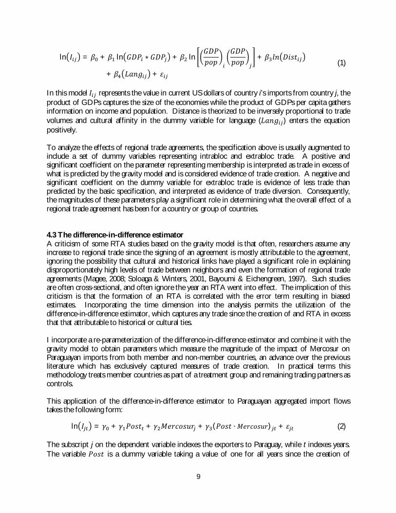
ln 퐼 = 훽 + 훽 ln 퐺퐷푃 ∗ 퐺퐷푃 + 훽 ln퐺퐷푃푝표푝

퐺퐷푃푝표푝 + 훽 푙푛 퐷푖푠푡

+ 훽 퐿푎푛푔 + 휀 (1)

In this model 퐼 represents the value in current US dollars of country i’s imports from country j, the product of GDPs captures the size of the economies while the product of GDPs per capita gathers information on income and population. Distance is theorized to be inversely proportional to trade volumes and cultural affinity in the dummy variable for language (퐿푎푛푔 ) enters the equation positively. To analyze the effects of regional trade agreements, the specification above is usually augmented to include a set of dummy variables representing intrabloc and extrabloc trade. A positive and significant coefficient on the parameter representing membership is interpreted as trade in excess of what is predicted by the gravity model and is considered evidence of trade creation. A negative and significant coefficient on the dummy variable for extrabloc trade is evidence of less trade than predicted by the basic specification, and interpreted as evidence of trade diversion. Consequently, the magnitudes of these parameters play a significant role in determining what the overall effect of a regional trade agreement has been for a country or group of countries. 4.3 The difference-in-difference estimator A criticism of some RTA studies based on the gravity model is that often, researchers assume any increase to regional trade since the signing of an agreement is mostly attributable to the agreement, ignoring the possibility that cultural and historical links have played a significant role in explaining disproportionately high levels of trade between neighbors and even the formation of regional trade agreements (Magee, 2008; Soloaga & Winters, 2001, Bayoumi & Eichengreen, 1997). Such studies are often cross-sectional, and often ignore the year an RTA went into effect. The implication of this criticism is that the formation of an RTA is correlated with the error term resulting in biased estimates. Incorporating the time dimension into the analysis permits the utilization of the difference-in-difference estimator, which captures any trade since the creation of and RTA in excess that that attributable to historical or cultural ties. I incorporate a re-parameterization of the difference-in-difference estimator and combine it with the gravity model to obtain parameters which measure the magnitude of the impact of Mercosur on Paraguayan imports from both member and non-member countries, an advance over the previous literature which has exclusively captured measures of trade creation. In practical terms this methodology treats member countries as part of a treatment group and remaining trading partners as controls. This application of the difference-in-difference estimator to Paraguayan aggregated import flows takes the following form:

ln 퐼 = 훾 + 훾 푃표푠푡 + 훾 푀푒푟푐표푠푢푟 + 훾 (푃표푠푡 ∙푀푒푟푐표푠푢푟) + 휀 (2) The subscript j on the dependent variable indexes the exporters to Paraguay, while t indexes years. The variable 푃표푠푡 is a dummy variable taking a value of one for all years since the creation of

10

Mercosur. The variable 푀푒푟푐표푠푢푟 (푀) takes a value of one for all Mercosur member countries for all years. Finally, 푃표푠푡 ∙푀푒푟푐표푠푢푟 (푃푀) is the interaction of these two dummy variables and consequently, 훾 is the average treatment effect of the Mercosur policy variable. The variable PM takes on a value of one for all Mercosur countries since the creation of Mercosur. That is, the variable PM represents membership to Mercosur, so I will use Members and PM interchangeably from here on. After exponentiating5 PM, it represents the average percent change in imports from non-member countries subtracted from the average percent change in imports from member countries for two given periods. More formally,

훾 = ln(퐼 ) − ln(퐼 ) − ln(퐼 ) − ln(퐼 ) (3) where the subscript M refers to Mercosur countries and NM to non-Mercosur countries, while the subscripts 1 and 2 refer to the years before and after the creation of Mercosur, respectively. The concepts of trade creation and trade diversion are implicit in 훾 of the expression above. To make these concepts explicit I reparameterized the difference-in-difference specification in (2) as follows:

ln 퐼 = 훾 + 훾 푀 + 훾 (푃푀) + 훾 (푃푁푀) + 휀푗푡 (4) where M and PM have been previously defined and PNM (푃표푠푡 ∙ 푁표푛푀푒푟푐표푠푢푟 ) takes on a value of one for Non-member countries since Mercosur’s creation. This is justified given the previously defined dummy variable Post is a linear combination of PM and PNM

푃표푠푡 = (푃푀)푗푡 + (푃푁푀) . (5) This decomposition of the dummy variable 푃표푠푡 will facilitate the identification of the average percent change in import flows from member and non-member countries since Mercosur’s creation. The sum of variables 푃푀 and 푃푁푀 capture aggregate factors that would affect trade flows even if Mercosur had not been created (Wooldridge, 2002). Hence, in the reparameterized form (4), the coefficients have the following interpretation:

훾 = ln(퐼 ) − ln(퐼 ) (6)

훾 = ln(퐼 ) − ln(퐼 ) (7) The benefit of this methodology is that difference-in-difference estimators control for unobserved factors determining high or low levels of bilateral trade among members of an RTA. It is an inflexible control for the passage of time, because as specified, 푃푀 and 푃푁푀 pool several years together. In sum, 훾 and 훾 capture changes in the levels of trade net of any historical or cultural link. I estimate a benchmark pooled cross-sectional Ordinary Least Squares (OLS) model taking the following form:

5 The exact percent change in the predicted value of 퐼 when 푃표푠푡 ∙ 푀푒푟푐표푠푢푟=1 versus when 푃표푠푡 ∙ 푀푒푟푐표푠푢푟=0 is given by 100(푒 − 1).

11

ln (퐼 ) = 훽 + 훽 푡 + 훽 ln 퐺퐷푃 ∙ 퐺퐷푃 + 훽 ln퐺퐷푃푝표푝

퐺퐷푃푝표푝

+ 훽 푙푛 퐷푖푠푡 + 훽 퐴푟푒푎 + 훽 퐿푎푛푔 + 훾 푀 + 훾 푃푀+ 훾 푃푁푀 + 휀

(8)

Recall the data are at the one digit level of commodity disaggregation. Hence, the additional subscript k is introduced to index commodities6. Considering only imports into Paraguay are analyzed, the subscript j indexes exporting countries and Py reflects Paraguayan values. Parameter 훽 − 훽 reflect the gravity and additional variables used to predict ‘natural’ flows of trade from the rest of the world to Paraguay. The last three parameters in (8), 훾 − 훾 , reflect the re-parameterization of the difference-in-difference estimator used to capture measures of trade creation and trade diversion. I use 1995 as the beginning year of Mercosur considering it was the year regional trade was originally planned to be liberated, as well as when convergence to the common external tariff began. An additional parameter in (8) is 훽 , the linear time trend coefficient. It is included in the specification to capture trending factors such as global inflation and growth. The usual method to do this is by including year fixed effects. However, in order to keep the difference estimators 훾 and 훾 in equation (8), it is not possible to include year dummy variables because the year fixed effects starting in 1995 form a linear combination with the dummy variables 푃푀 and 푃푁푀 . All models are estimated using robust standard errors in order to correct for serial correlation and heteroskedasticity in the error terms (Wooldridge, 2002). 4.4 Zero trade flow in trade data This data set is made of import flows from the rest of the world to Paraguay from 1970-2010. There are a total of 155 countries that export to Paraguay in at least one year and one commodity during this time. Consequently, after imputing the ‘missing’ observations into the data as zero trade flows, these represent 79% of the observations. As Frankel (1997) explains, missing values in a data set are attributable to little expected trade between countries because of size of the economies and remoteness from each other. Considering Paraguay is a small landlocked country and the trade values are at the one-digit level of detail, it is highly likely many countries will not export to Paraguay in all commodity codes in all years. I follow the traditional method of treating missing trade flows as the absence of trade between countries and treat these observations as zero trade flows. Econometrically, zero flows of trade represent a methodological challenge since the natural logarithm of zero is undefined. The literature describes several methods of dealing with zero trade flows. A very common approach is to ignore these missing observations. Frankel (1997), Fukao et al. (2003) explain this is what they have done in their study and it is likely Clausing (2001) also followed this approach considering the data in her study was rich in detail. Other techniques include substituting arbitrary small numbers for the zeroes, such as $1,000, or in constructing the dependent variable taking the natural log of the value of imports plus one. A third approach in dealing with this problem is using a Tobit model given trade values are bounded from below by zero. This is the approach followed by Soloaga & Winters (2001). However, the appropriateness of using the Tobit model has been questioned by Linders & de Groot (2006) on the basis the Tobit model would be

6 There are ten commodity codes ranging from 0 to 9.

12

justified if the censored data reflected negative trade values, or if the dependent variable existed but was unobservable. Frankel (1997) justifies the omission of the zero trade flows arguing the final results are not very sensitive to insertion of zero flows of trade. Soloaga & Winters (2001) make the same argument, claiming their results are robust to either the Tobit approach or the more traditional OLS methods omitting the zero flows of trade. The main concern with ignoring the zero trade flows is that results based on this approach may be biased. More recently, two widely cited approaches have been developed to handle the problem of zero trade flows. One solution is estimating the model using the import values measured in levels and implementing a Poisson maximum-likelihood estimator, traditionally used in estimating count regression models (Silvia and Tenreyro, 2006). This is the approach followed in some of the models in Magee (2008). The second approach treats the existence of zero trade flows as a sample selection problem and relies on the implementation of the Heckman two-step procedure for sample selection correction (Helpman et al. 2008; Linders & de Groot, 2006). I follow the second approach in this paper for a couple of reasons. First, considering Paraguay’s geographic location, landlocked condition, and developing country status are likely to limit Paraguay’s trading capacity, the Heckman model incorporates the probability of trading events to be realized conditioned on country characteristics. 4.4.1 Heckman Sample Selection Model in a gravity application Traditionally, data sets hold information on positive bilateral trade only. Occurrences of missing trade are discarded which is consistent with a sample selection problem. In this application, countries self-select into the sample by deciding to trade. Helpman et al. (2008) explains that by disregarding the missing or the inexistent flows of trade between countries, important information is ignored resulting in biased estimates. The Heckman two-step estimator is used to include the zero trade flows in this analysis and correct the sample selection problem. As its name suggests, this approach follows two steps. In the first stage or selection equation, the existence of a trading relationship is modeled using a probit model. Hence, the positive-valued trade observations take a value of one and all missing or zero-valued observations are censored at zero in the probit model. The predicted values of this model are used to construct the inverse Mills ratio, which is augmented to the outcome equation in the second stage, the gravity model in this application. The second stage or outcome equation is estimated on the uncensored observations only. This approach has several advantages. First, it adds flexibility to the comparable Tobit model, which restricts the censoring mechanism to be part of the outcome equation, the gravity model in this application. The two-step procedure models the processes separately. Using an OLS estimator in the second stage rather than maximum-likelihood methods permits the adoption of weaker distributional assumptions of the joint distribution of the error terms of both models (Cameron and Travedi, 2005). A priori, any potential correlation between the error terms of the first and second stages can be verified and corrected by this procedure. A lack of correlation between the error terms Cov(휀 , 푢 )=0, is indicative of no sample selection bias. Notice 휀 refers to the error term of the model prior to the implementation of the correction procedure.

13

Consequently, I estimate the following model:

Selection Equation:

푇 = 훽 + 훽 푡 + 훽 log 퐺퐷푃 ∙ 퐺퐷푃 + 훽 log퐺퐷푃푝표푝

퐺퐷푃푝표푝

+ 훽 푙표푔 퐷푖푠푡 + 훽 퐴푟푒푎 + 훽 퐿푎푛푔 + 훽 푅푒푙 + 훾 푀+ 훾 푃푀 + 훾 푃푁푀 + 푢

푇 = 1 푇푟푎푑푒 푉표푙푢푚푒 > 00 푇푟푎푑푒 푉표푙푢푚푒 = 0

Outcome Equation:

ln (퐼 ) = 훽 + 훽 푡 + 훽 log 퐺퐷푃 ∙ 퐺퐷푃 + 훽 log퐺퐷푃푝표푝

퐺퐷푃푝표푝

+ 훽 푙표푔 퐷푖푠푡 + 훽 퐴푟푒푎 + 훽 퐿푎푛푔 + 훾 푀 + 훾 푃푀+ 훾 푃푁푀 + 휆(푇 ) + 휃

(9)

All of the variables in (9) have been discussed except 푅푒푙 in the selection equation. This variable represents an index for religious similarity between trading partners. The higher the index the more similar the trading partners. It is included in the selection equation to meet the exclusion restriction recommended for two-part Heckman models such as (9)7. The exclusion restriction requires a variable to be correlated with inclusion in the sample (dependent variable in the selection equation), but uncorrelated with the error term in the outcome equation. That is, to meet the exclusion restriction requirements ‘religion’ should be positively related with the probability of countries trading with each other, but it should be uncorrelated with volume of trade in the outcome equation. This is also the variable suggested and used as an exclusion restriction in Helpman et al. (2008), which is by the author’s account, mostly a methodological paper developing an estimation procedure that corrects for potential biases in standard gravity equations. Additionally, the outcome equation includes the inverse Mills ratio 휆 푇 . This is the variable included in the gravity model to correct for sample selection bias. A statistically significant coefficient on this variable is consistent with evidence of sample selection bias. 4.4.1 Bias from time invariant unobserved country specific factors The significance of controlling for unobserved factors which may contribute to explain why a pair of countries might have a high or low levels of bilateral trade was discussed to be one of the benefits of using the difference-in-difference estimator in the gravity model environment. Although the 7 Both Cameron & Travedi (2005) and Wooldridge (2002) explain that both stages may be run using the same regressors omitting the exclusion restriction, but doing so risks the identification of the model and multicollinearity issues in the outcome equation due to an approximately linear inverse Mills ratio term over a wide range of arguments. However, this problem is attenuated by greater variation in the participation model. In this application the estimates are insensitive to whether an excluded variable is incorporated or not. Interestingly, Linders & de Groot (2006) apply a two-step Heckman selection model with maximum likelihood on the same set of regressors for each stage.

14

difference-in-difference estimator controls for these unobserved factors of member countries it does not control for unobserved factors explaining excess or limited trade with non-member countries. Introducing country fixed effects to the model will removes country-level heterogeneity bias associated with time invariant unobserved factors affecting the flows with all countries. The Heckman model now takes the following form:

Selection Equation:

푇 = 훽 + 훽 푡 + 훽 log 퐺퐷푃 ∙ 퐺퐷푃 + 훽 log + 훾 푃푀 +

훾 푃푁푀 + 퐶 + ⋯+ 퐶 + 푢 for 푗 = 1, … ,푁

푇 = 1 푇푟푎푑푒 푉표푙푢푚푒 > 00 푇푟푎푑푒 푉표푙푢푚푒 = 0

Outcome Equation:

ln (퐼 ) = 훽 + 훽 푡 + 훽 log 퐺퐷푃 ∙ 퐺퐷푃 + 훽 log +

훾 푃푀 + 훾 푃푁푀 + 휆 푇 + 퐶 + ⋯+ 퐶 + 휃 for 푗 = 1, … ,푁

(10)

The country fixed effects are reflected in the 퐶 dummy variables for N countries. This methodology significantly changes the original proposed specification considering time invariant variables can no longer be included in the model. In addition to controlling for time invariant factors affecting trade, including these fixed effects reduces the possibility that the researcher’s prior beliefs influence the specification of the gravity model Magee (2008). Several references recommend this technique for gravity model estimation (Matyas, 1997; Anderson & Van Wincoop, 2003; Baldwin et al., 2006; Helpman et al., 2008). As before, a pooled OLS country fixed effects model is included in the table of results. 5. Results Before reporting the main regression results I provide a glance at the structure of Paraguayan import values from 1970-2010. Table 1 reports the value and share of zero valued trade flows included in the data set. Clearly, the group of observations that may be categorized as manufactured merchandise has the highest number of positive trade value frequencies with respect to the potential number of observations8. ‘S1-6 Manufactured goods classified chiefly by material’, ‘S1-7 Machinery and transport equipment’, and ‘S1-8 Miscellaneous manufactured articles’ all have ratios of censored observations or zero trade flows below 70%. By no coincidence, they are also the categories of greatest import values only clearly surpassed by ‘S1-3 Mineral fuels’. This data is consistent with the structure of the Paraguayan economy being an exporter of mainly agricultural products. 8 The total number of potential observations for each commodity category is given by the number of countries by the number of years (41X155)=6355.

15

Table 1 Total value of Paraguayan imports by commodity in constant 2005 $US, 1970-2010.

Category Code Commodity Description

Censored

Share Imports

(millions) S1-0 Food and live animals 81% 4,432 S1-1 Beverages and tobacco 82% 6,477 S1-2 Crude materials, inedible, except fuels 81% 1,140 S1-3 Mineral fuels, lubricants and related materials 87% 14,185 S1-4 Animal and vegetable oils and fats 94% 112 S1-5 Chemicals 71% 11,794 S1-6 Manufactured goods classified chiefly by material 69% 11,584 S1-7 Machinery and transport equipment 68% 33,355 S1-8 Miscellaneous manufactured articles 67% 10,160 S1-9 Commod. & transacts. Not class. Accord. To kind 91% 128

Source: UN Comtrade database.

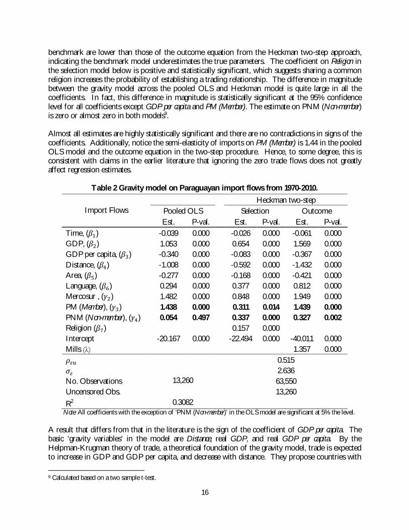
In the following section two sets of results are reported. The first set omits country fixed effects while the second set includes them, controlling for country-level heterogeneity. Each set holds pooled OLS and Heckman sample selection specification. The Heckman procedure and country fixed effects each correct a specific kind of bias, sample selection and heterogeneity, respectively. The results suggest the impact of Mercosur on Paraguayan imports flows is less sensitive to sample selection than heterogeneity bias. The estimates of the average percent increase in imports from members since the creation of Mercosur is consistently 322% in the first set of models that account for selection bias but ignore country-level heterogeneity (Table 2). Once heterogeneity is also accounted for, this figure is reduced to 267%. Consequently, omitting country fixed effects from the Heckman model overestimates member imports. Interestingly, it also underestimates non-member imports. Finally, I find evidence of trade creation in Beverages and Tobacco and Animal and vegetable oils & fat. Contrary to theory, we find no clear evidence of trade diversion. 5.1 Two Step Heckman Procedure The first set of results presented is a comparison of specifications (7) and (8) described in the previous section. This comparison will quantify the extent of bias attributable to sample selection. The results are presented in Table 2 below. As discussed earlier, any correlation between the error terms of the selection and outcome equation prior to correction, suggests estimates ignoring sample selection will be biased. The output suggests the error terms between the selection and outcome equations are positively correlated, Cov(휀 ,푢 )=0.515. Similarly, a standard t-test on the coefficient of the of the inverse Mills ratio (λ), is a valid test of the null hypothesis of no selection bias (Wooldridge, 2002). Given the coefficient is statistically significant at the 99% confidence level, this hypothesis is rejected. Inspecting the coefficient estimates on the outcome model and the benchmark, standard gravity model based on pooled OLS regression reveals that the magnitude of all coefficients of the

16

benchmark are lower than those of the outcome equation from the Heckman two-step approach, indicating the benchmark model underestimates the true parameters. The coefficient on Religion in the selection model below is positive and statistically significant, which suggests sharing a common religion increases the probability of establishing a trading relationship. The difference in magnitude between the gravity model across the pooled OLS and Heckman model is quite large in all the coefficients. In fact, this difference in magnitude is statistically significant at the 95% confidence level for all coefficients except GDP per capita and PM (Member). The estimate on PNM (Non-member) is zero or almost zero in both models9. Almost all estimates are highly statistically significant and there are no contradictions in signs of the coefficients. Additionally, notice the semi-elasticity of imports on PM (Member) is 1.44 in the pooled OLS model and the outcome equation in the two-step procedure. Hence, to some degree, this is consistent with claims in the earlier literature that ignoring the zero trade flows does not greatly affect regression estimates.

Table 2 Gravity model on Paraguayan import flows from 1970-2010.

Import Flows Heckman two-step

Pooled OLS Selection Outcome Est. P-val. Est. P-val. Est. P-val.

Time, (훽 ) -0.039 0.000 -0.026 0.000 -0.061 0.000 GDP, (훽 ) 1.053 0.000 0.654 0.000 1.569 0.000 GDP per capita, (훽 ) -0.340 0.000 -0.083 0.000 -0.367 0.000 Distance, (훽 ) -1.008 0.000 -0.592 0.000 -1.432 0.000 Area, (훽 ) -0.277 0.000 -0.168 0.000 -0.421 0.000 Language, (훽 ) 0.294 0.000 0.377 0.000 0.812 0.000 Mercosur , (훾 ) 1.482 0.000 0.848 0.000 1.949 0.000 PM (Member), (훾 ) 1.438 0.000 0.311 0.014 1.439 0.000 PNM (Non-member), (훾 ) 0.054 0.497 0.337 0.000 0.327 0.002 Religion (훽 ) 0.157 0.000 Intercept -20.167 0.000 -22.494 0.000 -40.011 0.000 Mills (λ) 1.357 0.000 휌 0.515 휎 2.636 No. Observations 13,260 63,550 Uncensored Obs. 13,260 R2 0.3082

Note: All coefficients with the exception of ‘PNM (Non-member)’ in the OLS model are significant at 5% the level. A result that differs from that in the literature is the sign of the coefficient of GDP per capita. The basic ‘gravity variables’ in the model are Distance, real GDP, and real GDP per capita. By the Helpman-Krugman theory of trade, a theoretical foundation of the gravity model, trade is expected to increase in GDP and GDP per capita, and decrease with distance. They propose countries with 9 Calculated based on a two sample t-test.

17

similar levels of productivity, as measured by GDP per capita, will trade more than countries with dissimilar levels (Frankel, 1997). Hence, developed countries with high GDPs per capita are more likely to trade with each other, which is usually reflected in a positive coefficient on GDP per capita. However, Paraguay’s context is entirely different. A negative and statistically significant coefficient on GDP per capita is consistent with the derivation of the gravity model based on the Heckscher-Ohlin theory of trade (Frankel, 2007). By this theory, countries export resource-abundant products while they import resource-scarce varieties. Merchandise trade can be described to be made up of capital, land, and labor-intensive products. Similarly, countries with high capital endowments are likely to have higher wages due to the higher labor productivity levels. Higher wages are reflected in higher GDP per capita levels and taking GDP per capita as a price signal, imports are expected to fall in GDP per capita, as they do in this application. This coefficient may be thought of as a price-elasticity of import demand. The coefficient on GDP per capita, -0.367 in the outcome equation, is consistent with an income inelasticity of import demand. The underestimation of the benchmark model is most evident on the coefficient for real GDP in Table 2. The GDP estimate in the outcome equation is greater than the benchmark by 0.51%. Land area, a proxy for resource endowment, has the expected negative sign. Its estimate in the outcome equation suggests imports decrease by 0.42% for every percent increase in land area. The negative sign is expected because larger countries are less dependent on international trade. A series of binary variables follow in the specification including the difference-in-different related parameters. First, I estimate that having a common language increases trade in the outcome equation by 125%10. Next, the difference-in-difference related coefficients are informative on how the creation of Mercosur has affected import flows to Paraguay since the initial year regional trade was planned to be liberalized, 1995. The Mercosur variable captures historical time invariant factors affecting regional imports which are likely to make regional imports disproportionately high. This estimate is 1.949 in the outcome equation of the Heckman model, quite greater than the estimate on the benchmark 1.482. The estimate on this coefficient in the outcome model implies regional factors increase trade by an average of 602% than predicted by the basic gravity variables. This gives an idea of how disproportionate significance of Mercosur countries in Paraguay’s import market. Interestingly, magnitudes of the difference estimators across the Heckman and the pooled OLS model are very similar, implying these estimates are quite insensitive to sample selection bias. The estimate on Members is interpreted as the average percent increase in imports from Mercosur countries since 1995. Hence, by the Heckman model imports from Mercosur countries have increased by a factor of 1.438 or 322% since 1995. Over the same period of time, imports from the rest of the world increased by 39%, as calculated from the estimate on Non-Members. The estimate on Non-Members in the benchmark model is lower (5.6%) and not statistically significant. The intercept in the difference-in-difference model is interpreted as the mean value of the dependent variable for the base group. In this case, the base group is made up of non-member countries in the years prior to Mercosur. However, considering the difference-in-difference estimator is estimated along with the gravity model, its interpretation is not as clear. Bayoumi and Eichengreen (1997) give an explanation of the intercept in the gravity model as representing greater

10 100 *(푒 . − 1).

18

than proportional growth in trade with respect to GDP if the constant is negative, as it is in this model.

Although the estimates on the Members and Non-Member across the models are qualitatively different, considering the coefficient on Non-Member is not statistically significant in the benchmark OLS model, they do not contradict each other. By these results, there is evidence of trade creation in Paraguay as a result of Mercosur. Regional trade has categorically increased since 1995 and the results do not suggest this increased regional trade has come at the expense of imports from the rest of the world. Imports from the rest of the world have also increased by the results in the Heckman model, and they are at least unchanged according to the benchmark model. The coefficients on Non-Member would have to be negative and statistically significant to support an argument for trade diversion in Paraguay.

Similarly, in a separate set of unreported estimation results, I calculated the proper difference-in-difference estimator or average treatment effect of Mercosur for both sets of models presented in Table 2. This estimate corresponds to 훾 in equation (2). Its values are in line with the findings thus far. The estimates in both models are statistically significant at the 95% confidence levels. Their values are 1.38 and 1.11 in the OLS and Heckman outcome equation, respectively. A two sample t-test yields the difference in these coefficients is not statistically significant. This result is also taken as evidence of trade creation since the magnitude of the coefficients indicates imports from regional partners have not been realized at the expense of imports from non-member. 5.2 Sensitivity Analysis using Country Fixed Effects A shortcoming of the difference-in-difference methodology reported previously is that unobserved time invariant factors that may affect levels of trade of non-member countries are not controlled for. These unobserved factors may also introduce bias in the estimates and a common approach used to address this issue is by estimating the model using country fixed effects. Unobserved and observed time invariant variables are differenced out of the model in this approach and consequently, the list of explanatory variables is reduced to only the time-varying variables. However, the interpretation of the difference estimators Member and Non-Member remains unchanged. As in the previous exercise, I estimate a benchmark pooled OLS model with country fixed effects along with the Heckman two-step model, also with country fixed effects. Several variables are removed from the model due to their time invariance including Distance, Area, Language, and Mercosur. The variable Religion is also removed from the selection equation in the two-step procedure since the index for religion is also time-invariant. The results are reported in Table 3. First, these results are consistent with previous estimates in that once again there is evidence of sample selection bias. The estimate on the Inverse Mills ratio in the two-step procedure is significant at levels higher than the 95% confidence level, justifying the sample selection correction. As before, the correlation between the error terms of the selection and outcome equations in the two step procedure have a positive correlation of Cov(휀 , 푢 )=0.632. Moreover, as in the previous set of results, the estimates in the benchmark model are an underestimate of the outcome equation in the Heckman model. The estimates in the benchmark model and the outcome equation in the two-step procedure are significant at the 95% confidence level except the coefficient on Non-Member in the benchmark.

19

The first notable difference between the results reported in Table 2 and Table 3 is that the difference in magnitude of the coefficients for GDP and GDP per capita has decreased after accounting for country fixed effects. In 훽 , 훽 , and 훽 of Table 3, the magnitude of the coefficients is greater in the Heckman model, suggesting that ignoring the zero trade values underestimates their true value. Interestingly, this same pattern does not hold when analyzing the coefficient reflecting regional or member imports. However, these differences in coefficients are not statistically significant at the 95% confidence level indicating the fixed effects model is insensitive to the inclusion of the zero trade flows.

Table 3 Fixed effects estimation results, Paraguayan import flows from 1970-2010. Heckman two-step

Import Flows Pooled OLS Selection Outcome β P-val. β P-val. β P-val. Time (훽 ) -0.102*** 0.000 -0.002 0.514 -0.119*** 0.000 GDP (훽 ) 2.484*** 0.000 0.362*** 0.000 3.172*** 0.000 GDP per Cap. (훽 ) -1.272** 0.010 -0.093 0.165 -1.664*** 0.000 PM, Member (훾 ) 1.440*** 0.000 0.116 0.371 1.299*** 0.000 PNM, Non-member (훾 ) 0.159* 0.088 0.281*** 0.000 0.410*** 0.000 Intercept -85.202*** 0.000 -17.807 0.000 -114.53*** 0.000 Mills (λ) 1.624*** 0.000 Country Fixed Effects Yes Yes Yes 휌 0.632 휎 2.567 Observations 13,260 63,550 Uncensored Obs. 13,260 Overall R2 0.1529

Note: *, **, *** imply significance at the 10%, 5%, and 1% levels, respectively. Gravity models without country fixed effects have been suspected of overestimating the impact of regional trade agreements. The reason being, without country fixed effects the model does not control for historical unobserved factors which might explain unusually high levels of trade between neighboring countries. Although I argued the difference-in-difference approach discussed in the previous section controls for these unobserved member specific factors, including country fixed effects reduces the membership estimates from about 1.440 in both OLS models and the Heckman approach without fixed effects, to 1.299 in the two step procedure with country fixed effects. This figure represents a change in average increase of Mercosur imports from 322% in outcome equation of Table 2 to 266% in Table 3. Moreover, including country fixed effects reveals a higher magnitude of increase in average imports from non-member countries with respect to both, the pooled OLS model with country fixed effects and the two step procedure without country fixed effects. Hence, omitting controls for country-level heterogeneity underestimates imports from non-member trading partners. The outcome equation in Table 3 indicates imports from non-members have increased by 50.7%, rather the than 38.6% figure estimated in the Heckman model omitting country fixed effects. Regardless of this

20

change in magnitude, the original interpretation of these results stands. There is no empirical evidence in the model sustaining that the increase in imports from regional partners has been offset by a decrease in imports from the rest of the world. These empirical results support a finding of trade creation in Paraguay. The average percent changes in imports based on the estimates of our main parameters of interest, ‘PM - Member (γ3)’ and ‘PNM Non-Member (γ4)’, of all implemented specifications are summarized in Table 4.

Table 4 Percent change in imports from member and non-member countries with and without fixed effects and by estimator.

Parameters No Fixed Effects Fixed Effects OLS Heckman OLS Heckman

PM, Member (γ3) 321.2%*** 321.6%*** 322.1%*** 266.5%*** PNM, Non-Member (γ4) 5.6% 38.6% 17.3%* 50.7%***

Note: *, **, *** imply significance of estimates at the 10%, 5%, and 1% levels, respectively. Regarding the average treatment effect of Mercosur on Paraguay using the parameterization of the gravity model consistent with equation (2) and country fixed effects, the unreported difference-in-difference estimators are 1.28 and 0.89 in the pooled OLS and Heckman models, respectively. Although the difference in magnitude is not statistically significant at the 95% confidence level, it is once again evidence that the sample selection procedure attenuates the magnitude of the OLS difference-in-difference estimator. The interpretation of the Heckman model is that membership to Mercosur has increased imports from the region net of the increase in imports from non-members an average of 143% since 1995 (260% using pooled OLS with fixed effects). Although this estimate is smaller than the specifications omitting fixed effects, this result continues to be consistent with trade creation.

5.2 Sector analysis using the pooled OLS model with fixed effects To make use of the richness of the data, the Heckman model with country fixed effects has also been estimated for trade flows at the commodity level. Table 5 introduces the results of ten regressions, each at the commodity level of disaggregation. The columns reported under Member and Non-Member are the coefficient estimates of the specification described by (10). Columns (3) and (4) report the exact percentage interpretations of the coefficient estimates in (1) and (2). The number of countries exporting to Paraguay within each commodity category and the number of observations are also reported in columns (5) and (6), respectively. The share of censored data for each regression is also reported in column (6). As discussed in Table 1, Table 5 shows that most import observations take place in the following manufactured commodity categories: Chemicals, Manufactured goods classified by materials, Machinery & transport equipment and Miscellaneous manufactured articles. Not only is the number of observations the greatest in these categories, but so is the number of exporting countries, giving an indication of the significance manufactured goods in imports. Though the coefficient for Member is statistically significant at least at the 90% confidence level in all regressions except Mineral Fuels & Lubricants, the coefficients for Non-Member are statistically significant for fewer classifications. In addition to being not statistically significant in Mineral Fuels & Lubricants, Non-Member is not significant in Food and Live Animals and Animal and vegetable oils & fats.

21

The greatest import expansions are observed in Beverages and Tobacco, and Animal and vegetable oils & fats11. The average percent increases in imports in these categories are, 3,816% and 5,325%, respectively. Although these import expansions reflect examples great trade creation, they are also commodities in which the common external tariff (CET) is effective. This implies these merchandise categories may be benefitting from certain protection. For example, beginning in 2006 the CET on vegetable oils has been applied at 10%. Additionally, the CET on tobacco and beverages ranges from 14-20% (Chapter 22 HS-2006 – Mercosur Secretariat). Although the greatest expansion of imports is in commodities where the CET is effective, they are also categories in which Paraguay also has a production capacity.

Table 5 Impacts of Mercosur on Paraguayan imports at the one digit SITC Rev. 1 level.

(1) (2) (3) (4) (5) (6)

Merchandise Description

Member (p-value)

Non- Member (p-value)

Member % Change

Non-Member

% Change Countries

Obs. (Censored

Ratio) S1-0 Food and live animals

1.103*** 0.136 201% 15% 72 2,952 (59%) (0.000) (0.398)

S1-1 Beverages and tobacco

3.668*** 0.391** 3,816% 48% 73 2, 993 (61%) (0.000) (0.018)

S1-2 Crude materials, inedible, except fuels

0.69* 0.394** 99% 48% 89 3,649 (66%) (0.079) (0.037)

S1-3 Mineral fuels and lubricants

0.219 -0.392 25% -32% 62 2,543 (69%) (0.665) (0.235)

S1-4 Animal and vegetable oils & fats

3.994*** -0.279 5,325% -24% 34 1,394 (73%) (0.000) (0.484)

S1-5 Chemicals 1.565*** 0.473*** 378% 61% 104 4,264 (57%) (0.000) (0.000)

S1-6 Manuf. goods classified by material

1.100*** 0.517*** 200% 68% 110 4,510 (56%) (0.000) (0.000)

S1-7 Machinery & transport equipment

0.563* 0.481*** 76% 62% 125 5,125 (61%) (0.057) (0.000)

S1-8 Miscellaneous manuf. articles

1.345*** 0.471*** 284% 60% 126 5,166 (60%) 0.000 0.000

S1-9 Commod. & transacts. Not class.

4.050*** 3.115*** 5,641% 2,153% 64 2,624 (79%) (0.001) (0.006)

Note: ***, **, and * denote significance at the 1%, 5%, and 10% levels, respectively. Additionally all Mercosur countries are recognized producers of primary goods such as those included under Animal and vegetable oils & fats. Furthermore, the coefficient on Non-Member for Beverages and Tobacco, and Animal and vegetable oils & fats is positive and statistically significant for the former and negative but not statistically significant for the latter. These results attenuate the claim of trade diversion and actually support the argument of trade creation. A similar primary product

11 The category Commodities & transactions not classified according to kind. also encountered a great expansion but is not discussed due to the vague description of the merchandise included in this category.

22

category such as Food and Live Animals also exhibited increases in both regional and international imports by 201% and 15%, respectively, results which are also consistent with trade creation. Imports in manufactured goods have also expanded significantly, especially Chemicals and Miscellaneous manufactured articles. Imports in these products have increased by 378% and 284%, respectively. Imports from non-member countries have also increase by 61% and 68%, respectively. The same is true of Manufactured goods classified by material and Machinery & transportation equipment which have experienced statistically significant regional and extra-regional import expansions since 1995, denying any claim of overall trade diversion. Recall, it is in the manufactured good categories where there are numerous exemptions to the CET, especially in capital goods and information and communication technology equipment. 6. Conclusions In this paper I used the gravity model of international trade to analyze how the creation of Mercosur has affected import flows into Paraguay. In order to account for zero trade flows I compared a benchmark pooled OLS model to an application of the Heckman model with and without country fixed effects. The Heckman model corrected an underestimation of ‘gravity’ variables in the pooled OLS estimates attributed to sample selection bias. However, there was no noticeable difference in the impact of membership to Mercosur between these two models. Including country fixed effects in the model decreased this estimate (PM-Member) and increased the estimate for imports from the rest of the world (PNM - Non-member). This result highlights the significance of correcting for time invariant bilateral trading characteristic across all countries. That is, heterogeneity bias had a greater influence than selection bias in the policy variable in these results. Although I outlined a conceptual framework where I anticipated finding evidence of trade diversion in Paraguay, the empirical results did not support this claim in the aggregate or commodity level trade values. Quite the opposite, I found evidence of trade creation in all commodity categories. The only commodities where a decrease in imports from non-member countries is observed are Mineral fuels and lubricants and Animal and vegetable oils & fat, but these estimates are not statistically significant. The most disproportional increases in import levels from member countries were observed in Beverages and Tobacco and Animal and vegetable oils & fat. Considering the CET is in effect in these categories and is as high as 20% for some products (Mercosur-Secretariat), it is possible some trade diversion may have taken place. However, Paraguay has a production capacity in these categories and their import expansion attributable to Mercosur overwhelmingly outweighs the negligible losses attributable to trade diversion. Such developments are clearly beneficial. The expansion in imports of manufactured goods from Mercosur is less disproportionate and is possibly attenuated by the fact that many products in this sector are still exempt from the CET. Further research may illustrate how imports of non-exempt manufactured goods from the CET have been affected by Mercosur. Looking forward, it is likely Paraguay’s policy will be to continue supporting the benefits obtained in the agricultural sector, but to keep postponing the application of the CET on high technology manufactured goods.

23

7. Appendix

Table A.1 Exporting Countries to Paraguay 1970-2010 Afghanistan Denmark Kyrgyzstan Russian Federation Albania Dominica Lao People's Dem. Rep. Rwanda Algeria Dominican Rep. Latvia Saudi Arabia Angola Ecuador Lebanon Senegal Argentina Egypt Lesotho Serbia Australia El Salvador Liberia Sierra Leone Austria Equatorial Guinea Libya Singapore Bahamas Estonia Lithuania Slovakia Bahrain Ethiopia Luxembourg Slovenia Bangladesh Finland Madagascar South Africa Barbados France Malaysia Spain Belarus French Polynesia Malta Sri Lanka Belgium FS Micronesia Mauritania Sudan Belize Gabon Mauritius Suriname Bermuda Gambia Mexico Swaziland Bolivia Georgia Mongolia Sweden Bosnia Herzegovina Germany Morocco Switzerland Botswana Ghana Mozambique Syria Brazil Greece Myanmar Tajikistan Brunei Darussalam Grenada Namibia TFYR of Macedonia Bulgaria Guatemala Nepal Thailand Burundi Guinea Netherlands Togo Cambodia Guyana New Caledonia Trinidad and Tobago Cameroon Haiti New Zealand Tunisia Canada Honduras Nicaragua Turkey Central African Rep. Hungary Niger Turkmenistan Chile Iceland Nigeria Uganda China India Norway Ukraine China, Hong Kong Indonesia Occ. Palestinian Terr. United Arab Emirates China, Macao SAR Iran Oman United Kingdom Colombia Iraq Pakistan U. Rep. of Tanzania Congo Ireland Panama Uruguay Costa Rica Israel Peru USA Côte d'Ivoire Italy Philippines Uzbekistan Croatia Jamaica Poland Venezuela Cuba Japan Portugal Viet Nam Cyprus Jordan Rep. of Korea Yemen Czech Rep. Kenya Rep. Moldova Zimbabwe Dem. R. of Congo Kuwait Romania

24

8. References

Anderson, J., and E. van Wincoop. 2003. “Gravity with Gravitas: A Solution to the Border Puzzle.” Americkan Economic Review 93.

Baldwin, R. and D. Taglioni. 2006. “Gravity for Dummies and Dummies for Gravity.” NBER

working paper No. 23516, Cambridge, MA: National Bureau of Economic Research. Bayoumi, T., & Eichengreen, B. “Is regionalism simply a diversion? Evidence from the evolution of

the EC and EFTA.” Chapter 6, Regionalism versus Multilateral Trade Arrangements, Takatoshi Ito and Anne O. Krueger, editors. Chicago: University of Chicago Press, 1997

Berlinski Julio, Kume, Vaillant, Miranda, Ons, and Romero 2005, “Aranceles a las Importaciones en

el Mercosur: El Camino al Arancel Externo Comun” Departamento de Economia, Universidad de la Republica, Uruguay.

Bhagwati, Jadish. 1996. “Preferential Trading Areas and Multilateralism- Strangers, Friends, or

Foes?”. Chapter 2, Trading Blocs: Alternative Approaches to Analyzing Preferential Trade Agreements, Jadiwh Bhagwati, Pravin Krishna, and Arvind Panagariya, editors. Cambridge, MA” The MIT Press, 1999

Cameron, A. Colin and P. Travedi. 2005. Microeconometrics: Methods and Applications. New York, NY: Cambridge University Press.

Clausing, K. 2001. “Trade creation and trade diversion in the Canada – United States Free Trade

Agreement.” Canadian journal of Economics. 34(3). Deardorff, Alan. 1997. “Determinant of Bilateral Trade: Does Gravity Work in a Classical World?”

In The Regionalization of the World Economy, ed. by Jeffrey Frankel. Chicago: University of Chicago Press.

Frankel, Jeffrey A. 1997. Regional Trading Blocs in the World Economic System. Washington, DC: Institute

for International Economics. Fukao, Kyoji, Toshihiro Okubo, and Robert M. Stern. 2003. “An Econometric Analysis of Trade

Diversion under NAFTA.” North American Journal of Economics and Finance Vol. 14. Heckman J. 1979. “Sample Selection Bias as a Specification Error.” Econometrica. Vol. 47 (1). Helpman, E., Melitz, M., & Rubinstein Y. 2008. “Estimating Trade Flows: Trading Partners and

Trading Volumes.” The Quarterly Journal of Economics 123(2). Helpman, E. & Krugman P. 1985. “Politics and Trade Policy.” NBER Working Paper No. 5309.

Cambridge, MA: National Bureau of Economic Research. Krueger, Anne O. 1999. “Trade Creation and Trade Diversion under NAFTA.” National Bureau of

Economic Research, Working Paper 7429 (December).

25

Linders, Gert-Jan M. and Henri L.F. de Groot (2006). “Estimation of the Gravity Equation in the Presence of Zero Flows.” Tinbergen Institute Discussion Paper, 2006-072/3.

Magee, C. 2008. “New measures of trade creation and trade diversion.” Journal of International

Economics, 75 (2). Matyas, L. 1997. “Proper Econometric Specification of the Gravity Model.” The World Economy, 20. Santos Silva, J. M. C. and Tenreyro, S. (2006). “The Log of Gravity.” The Review of Economics and

Statistics, 88(4) Soloaga, Isidro and L. Alan Winters. 2001. “Regionalism in the Nineties: What Effect on Trade?”

North American Journal of Economics and Finance 12:1-29 Tinbergen,J. 1962. Shaping the World Economy: Suggestions for an international Economic Policy. The

Twentieth Century Fund, New York. Viner, Jacob. 1950. The Customs Union Issue. New York: Carnegie Endowment for International Peace Wooldridge, J. 2002. Econometric Analysis of Cross Section and Panel Data. Cambridge, MA: MIT Press. Yeats, Alexander J. 1998. “Does Mercosur’s Trade Performance Raise Concerns about the Effects

of Regional Trade Arrangements?” World Bank Economic Review Vol. 12, No.1