an econometric analysis of the role of financial ... · an econometric analysis of the role of...

This PDF is a selection from an out-of-print volume from the NationalBureau of Economic Research

Volume Title: Determinants of Investment Behavior

Volume Author/Editor: Robert Ferber, editor

Volume Publisher: NBER

Volume ISBN: 0-87014-309-3

Volume URL: http://www.nber.org/books/ferb67-1

Publication Date: 1967

Chapter Title: An Econometric Analysis of the Role of Financial Intermediaries in Postwar Residential Building Cycles

Chapter Author: Gordon Sparks

Chapter URL: http://www.nber.org/chapters/c1239

Chapter pages in book: (p. 301 - 331)

An Econometric Analysis of the Role

of Financial Intermediaries in

Postwar Residential Building Cycles

GORDON R. SPARKSUNIVERSITY OF MICHIGAN

The purpose of this paper is to develop a model of the residential con-struction sector of the U.S. economy, with particular emphasis on thefinancial factors that provide a link between construction activity and themonetary sector. The study was undertaken as part of a larger project toincorporate monetary policy variables into the econometric model con-structed by the Research Seminar in Quantitative Economics at theUniversity of Michigan.' As this is an annual model designed for short-run forecasting and policy analysis, the equations for the residentialconstruction sector have been estimated from postwar annual data.

Our model consists of a set of equations which determine the flowof funds through financial intermediaries and their influence on con-struction activity. The rate of accumulation of savings deposits isassumed to depend on interest rates and personal financial saving. Theinflow of deposits together with interest rates and other variables thendetermine the volume of commitments made by financial institutions

NOTE: This paper is based on a Ph.D. dissertation undertaken at the Universityof Michigan with financial support provided by a Ford Foundation fellowship.However, the conclusions, opinions, and other statements presented here are thoseof the author and not necessarily those of the Ford Foundation. I am indebted toDaniel B. Suits, James C. T. Mao, Harold T. Shapiro, Warren L. Smith, andRonald L. Teigen for their valuable comments.

1 For a description of this model, see [14] and [16]. Numbers in brackets refer toBibliography at end of paper.

302 Consumer Assets

to supply residential mortgage funds. The supply of mortgage commit-ments then affects housing starts and residential construction expendi-tures. Equations for housing starts and the supply of mortgage fundsare formulated in section I of the paper and the empirical results arepresented in section II. Equations for savings deposits are given in sec-tion III and the implications of the model for monetary policy are dis-cussed in section IV.

1. Housing Starts and the Mortgage MarketThe most striking feature of housing starts in the postwar period hasbeen the countercyclical behavior of this series. Building has typicallyrisen sharply during periods when the general level of economic activitywas approaching a cyclical trough. During the early stages of an upswing,housing starts have continued to increase but have reached a peak wellin advance of the peaks indicated by the National Bureau referencecycles.2 Most students of the housing market have considered the sup-ply of mortgage credit to be the major cause of this behavior. Forexample, Grebler3 gives the following characterization of postwar resi-dential building cycles: "Given long-run demand and supply forcesfavorable to residential building, short-run cycles in housing construc-tion were associated for the most part with changes in the supply ofmortgage funds and credit terms, which in turn were greatly influencedby the level of total economic activity. When that level was rising andhigh, the expanded demand for funds by business, which is relativelyinsensitive to increased cost of borrowing, tended to reduce the avail-ability of funds for housing, which is highly sensitive to changes in thecost of borrowing."

Among the proponents of this view, there has been some disagree-ment over the importance of the legal maximum interest rates on mort-gages insured by the Federal Housing Administration or guaranteed bythe Veterans Administration. Guttentag [6] argues that the effect of therate maxima has been greatly exaggerated. He emphasizes the demandside of the market for mortgage funds and argues that housing demandis more highly sensitive to changes in mortgage credit terms than tochanges in the flow of current income. A similar view is expressed byAlberts [1].

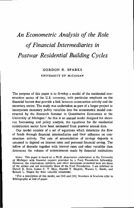
A graphical exposition of this theory is given in Figure 1. For pur-2 See [17], Chart 1A.

[5], p. 104.

Financial intermediaries in Building Cycles

FIGURE 1Allocation of Funds Between Mortgages and Bonds

303

ICorporate bonds

=

I

(1)

I I

I I

supplyI ..J

Mortgage funds

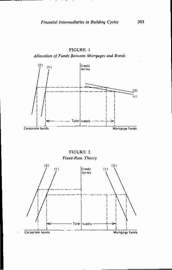
FIGURE 2Fixed-Rate Theory

Creditterms

supply

Corporate bonds Mortgage funds

Citterms

(2) (1)

Total —l

(2)(1)

(2)(1)

L Iota I

I I

—I•

I

I I I

304 Consumer Assets

poses of illustration, we assume a fixed supply of funds to be allocatedbetween corporate bonds and mortgages. The demand for mortgagefunds is assumed to be highly responsive to changes in credit termswhile the demand by corporations is assumed to be inelastic. A rise inincome causes both schedules to shift upward but has a greater effecton corporate demand, resulting in a shift of funds away from mortgages.4The fixed-rate theory, advanced by Warren Smith [15] and others, isifiustrated in Figure 2. According to this view, the spread between theceiling rates on insured and guaranteed mortgages and yields on othersecurities has an important influence on the supply of mortgage funds.Assuming that the interest rate is at the statutory maximum at the initialequilibrium, an upward shift in the schedules results in a reallocationof funds from mortgages to corporate bonds, leaving an excess demandin the mortgage market.

A rather different approach to the explanation of fluctuations in hous-ing starts is taken in a recent study by Maisel [12], who emphasizes theimportance of changes in vacancies and the inventory of houses underconstruction. According to his theory, the lag in the response of buildersto changes in demand and the lag between starts and completions leadto an inventory cycle. He includes among the determinants of housingstarts, vacancies at the beginning of the period, net household forma-tions, removals (from the housing stock), and the ratio of rents to con-struction costs as a measure of the income from building or owninghouses. As a measure of the cost and availability of credit, he uses alagged moving average of the Treasury bill rate. Maisel emphasizes thatthe impact of credit conditions is on the supply side of the housingmarket rather than on the demand side. He argues that there is littlerelationship between credit conditions and final demand as measured bynet household formations, but that changes in credit conditions influencethe willingness of builders to increase their inventories under construction.

We have attempted to combine Maisel's approach with a more detailedtreatment of the supply of mortgage funds. Housing starts (HS) areassumed to depend on the following variables.

1. Inventory of houses under construction plus vacancies at thebeginning of the period. In terms of first differences, the sum of thesetwo variables was represented by housing starts less net household forma-tions (HF), using the following identities and disregarding removals:

4 Denoting the credit elasticities of demand for corporate funds and mortgagesby ébc and emc, respectively, and the income elasticities by and emy, respectively,the condition for a shift of funds away from mortgages is ebc/emc < ebv/emv.

Financial Intermediaries in Building Cycles 305

(vacancies) equals completions minus net household formationsminus removals.

(inventories under construction) equals starts minus completions.2. Ratio of rents (R) to construction costs (C) at the beginning of

the period.3. Mortgage credit terms (Cr).4. Net household formations (HF). This variable was used with the

reservation that the available data supplied by the Bureau of the Censusis subject to considerable sampling variability [18]. As noted byMaisel [11], even the direction of change in net household formationsmay be in error.

5. Disposable income (Y). We have included an income variable asa determinant of the demand for owner-occupied as opposed to rentalunits. High income may stimulate the demand for home ownership andlead to an increase in single-unit starts. Total starts will be affected if,as is likely to be the case, there is a lag in the reaction to increasedvacancies of rental units. Assuming a linear relationship, our equationfor housing starts becomes

LiHS = ao — aj(HS — HF)_1 + —j.i — +

Since mortgage credit terms cannot be assumed to be exogenous tothe housing market, a model of the mortgage market is also required.The demand for residential mortgage funds comes from three sources:builders, investors in rental units, and individuals purchasing existing orcustom-built homes. The major sources of supply are the four main typesof financial intermediaries: savings and loan associations, mutual sav-ings banks, life insurance companies, and commercial banks—plus theFederal National Mortgage Association. An important institutional fea-ture of this market is the use of forward commitments under which aninvestor agrees to lend a specific amount of money at a given interestrate within a specified period of time. A residential builder generallyseeks a commitment for permanent mortgage financing from a financialinstitution before construction is begun. According to Klaman,5 com-mercial banks will usually make short-term loans to finance constructiononly after a builder has obtained such a commitment. Thus, the willing-ness of financial institutions to enter into forward commitments is likelyto have an important impact on housing starts. Accordingly, we haveformulated the demand for mortgage funds in terms of the demand for

[9], p. 168.

306 Consumer Assets

loans disbursed without prior commitment plus forward commitments.This variable, denoted by MC, is assumed to depend on the same factorsas housing starts. Thus, we have

= — — HF)_1 + — +

On the supply side of the mortgage market, our basic approach to theexplanation of the mortgage lending of financial intermediaries isexpressed by the following equation:

/= Yio + + — )....i —

SD1

+ l'5ACP?The volume of mortgage loans and commitments (MCi) made by the

lender is assumed to depend on the inflow of savings depositsand repayments on outstanding mortgages the ratio of mortgageholdings (Mi) to deposits at the beginning of the period, mortgagecredit terms (Cr), and a market rate of interest (r) which representsthe yield on alternative investments.

In order to avoid the problem of simultaneous-equation estimationbias, we solved the above model to obtain a reduced form equation forhousing starts, which did not contain the mortgage credit term variableexplicitly. This procedure has the additional advantage of eliminatingthe need for a quantitative measure of credit terms. The interest returnon mortgages is an inadequate indicator to the extent that changes incredit conditions are reflected in changes in loan-to-value ratios andmaturities.

Equating supply and demand in the mortgage market, we obtain

• +FNMA represents net purchases of mortgages by the

Federal National Mortgage Association. Substituting the supply anddemand functions, we obtain an equation from which an expression forthe variable can be derived as follows:

[l'jD + ± — ) — +\+

— — HF)_1 +'s—)

— + i34iXHF +\ C.__1


1 ( IR\= f3o — f31(HS — HF)_1 + 134 + +75483k \ Ci_1

/+ + — ) —\ SD1,'_1 /

where Substituting this expression in the housing startsequation we obtain

/R\a'o — — HF)_1 + + +C—i

( / M\+ [yio + + — J —\

+

where a, = a7 — ;j = 0, 1, 2, 4, 5; and a =75+133 75+133

Because of the limited number of degrees of freedom provided bypostwar annual data, the coefficients in the above equation were esti-mated in two stages. First the were estimated from regressions usingthe as the dependent variables.6 The a1 were then estimatedfrom a regression of housing starts on the estimated changes in the totalsupply of mortgage funds (MC + FNMA) along with the other inde-pendent variables appearing in the reduced form equation.7 The resultsof these regressions are reported in the next section.

8 These regressions do not represent the true reduced forms which would beobtained by substituting the expression derived above for in the equations forthe supply of mortgage funds. Since the expressions resulting from this substitutionwould contain all the exogenous variables in the model, a source of bias is intro-duced to the extent that the omitted exogenous variables are correlated with thoseincluded.

A reviewer of this paper has objected to the use of sixteen observations toestimate the more than sixteen parameters appearing in the above equation. Wehave simply followed the usual method of estimating the reduced form coefficientsin a simultaneous system and gained degrees of freedom by first obtaining directestimates of the structural coefficients Our procedure differs from a straight-forward application of two-stage least squares in that we have used the supply offunds in the first stage regressions rather than the credit term variable that appearsin the structural equations. Because of this modification we have not attempted toadjust the standard errors in the second-stage regression to take account of errorsin the estimates of the first-stage coefficients so that the former are likely to bebiased downward.

308 Consumer Assets

ii. Empirical ResultsSAVINGS AND LOAN ASSOCiATIONS

The regression results for mortgage lending of savings and loan asso-ciations are shown in Table 1. The values of the dependent variable MC1were computed as the sum of mortgage loans made (ML1) plus thechange in outstanding commitments during the year. Since no data onoutstanding commitments were available for the earlier years, the equa-tions were fitted to the period 1957—64.

As a measure of the rate of return on alternative investments, thelong-term U.S. rate was used since the nonmortgage security holdings ofsavings and loan associations consist mainly of U.S. government securi-ties.8 This variable did not obtain a significant coefficient as might beexpected from the institutional considerations. According to Klaman,9"Compared with other major financial institutions in the mortgagemarket, savings and loan associations are singularly limited by law andtradition to the specialized role of home mortgage lenders. In homemortgage markets they specialize, also, in providing conventional loansdirectly to individual borrowers in local markets and thus are less flexiblethan other financial institutions in adjusting investment programs tochanges in capital market conditions."

Between 1949 and 1963 the ratio of mortgage holdings to savings andloan shares varied within a fairly narrow range of 93 to 99 per centwhile the average annual increase in shares has been about 15 per cent,indiáating that the inflow of savings capital has been the major influenceon mortgage lending. In addition, at the end of 1963, conventional asopposed to government-insured or guaranteed mortgages made up 87 percent of total mortgage holdings. Thus, the ceiling rates have been oflittle importance.

The third equation in Table 1 was fitted with the coefficient on repay-ments constrained to be unity. The unconstrained coefficient obtainedseems unreasonable and is likely to be biased upward. During periodswhen the level of mortgage lending and construction is high, advancepayoffs of loans rise due to the sale of existing properties. Thus repay-ments are not exogenously determined but are influenced to some extentby the volume of mortgage loans made.

8 Federal associations are restricted by law from holding state and local govern-ment or private securities, and state-chartered institutions are subject to similarlimitations [4].

[9], p. 18.

TAB

LE 1

Mor

tgag

e Le

ndin

g of

Sav

ings

and

Loa

n A

ssoc

iatio

ns

-4.

Perio

d

Dep

ende

ntV

aria

ble

A2S

D1

(bill

. $)

(bill

. $)

/A

RE

P1

(bill

. $)

\S

D1)

1(p

er c

ent)

Con

stan

tTe

rmR

2df

1957

-64

AM

C1

1.10

61.

482

—44

.601

—.2

197

—.1

551

.969

3(.1

16)

(.141

)(1

1.06

7)(.5

789)

1957

-64

AM

C1

1.12

41.

487

—42

.840

—.2

028

.976

4(.0

94)

(.124

)(8

.908

)19

57-6

4A

MC

11.

090

1.00

0—

37.7

60.3

117

.905

5(.1

85)

(17.

342)

1949

-64

AM

L1.9

159

1.00

0—

27.9

14.2

633

.848

13(.1

836)

(9.1

91)

TAB

LE 2

Mor

tgag

e Lo

ans a

ndC

omm

itmen

ts o

f Mut

ual

Savi

ngs B

anks

,19

52 -6

4

A2S

D2

(bill

. $)

L\R

EP2

(A(b

ill.

$)\

SD

2/.1

ArC

b(p

erce

nt)

A(r

m-r

cb)

(per

cent

)C

onst

ant

Term

R2

df

1.22

6—

J086

—21

.215

—1.

338

.988

0.8

228

(.273

)(.7

686)

(11.

641)

(.762

)1.

230

—20

.787

—1.

331

.953

3.8

429

(.256

)(1

0.60

9)(.7

18)

1.33

1.6

203

—15

.076

•

1.63

6.5

374

.858

8(.2

05)

(.735

0)(1

1.16

9)(.6

74)

1.34

5—

19.

038

1.43

0.7

593

.863

9(.2

01)

(9.9

71)

(.618

)

g 0

310 Consumer Assets

Using a one-sided t-test with five degrees of freedom, both coefficientsin the constrained regression are significant at the 5 per cent level andthe coefficient on is significant at the 1 per cent level. Becauseof limited amount of data available on outstanding commitments, theequation was fitted to the period 1949—64, using as the dependentvariable. In this case, both coefficients are significant at the 1 per centlevel.

MUTUAL SAVINGS BANKS

In contrast to savings and loan associations, the portfolio regulationsand policies of mutual savings banks permit them to take advantage ofchanging yield differentials. The laws of the seventeeen states in whichmutual savings banks operate generally permit investment in bonds ofstate and local governments and corporations. Their portfolio choicesare likely to be responsive to the level of the ceiling rates on government-insured and guaranteed mortgages since a relatively high percentage oftheir mortgage holdings are FHA and VA loans and they have generallybeen reluctant to resort to discounting.'°

The equations were fitted to the period 1952—64 for which commit-ments data were available and the results are shown in Table 2. Thecorporate bond rate (rCb) was used to represent the rate on competingassets. Slightly better results were obtained using the differential betweenthe average of the FHA and VA ceiling rates (rm) and the corporatebond rate. In both cases, the repayments variable was not significant.

LIFE INSURANCE COMPANIES

Like mutual savings banks, life insurance companies have a wide degreeof flexibility in their choice of assets, but their responsiveness to short-run changes in available funds and yield differentials is limited by thepractice of planning ahead a year or more." They make extensive useof forward commitments which typically cover a time period from aboutthree months on existing homes to six to twelve months for new con-struction and up to two and a half years for apartment houses.'2

The regression results obtained for the period 1954—64 are shown inTable 3. The equations were fitted using the corporate bond rate andthe differential between the average of the FHA and VA ceiling ratesand the corporate bond rate. In contrast to the mutual savings bank

10 [4], p. 175.ii [9], Chapter 6.12 [10], p. 186.

TAB

LE3

Mor

tgag

e Lo

ans

and

Com

mitm

ents

of L

ife In

sura

nce

Com

pani

es, 1

954

-64

SD3

(bill

. $)

(bill

. s)

\S

D3/

-1

(per

cent

)A

(rm

—rc

b)(p

erce

nt)

Con

stan

tT

erm

R2

df

.660

6(.8

900)

—.1

708

(1.3

48)

—25

.178

(24.

008)

—2.

689

(.986

)1.

0313

.640

6

.596

6(.3

565)

-.2.8

39(.6

19)

.768

7.6

818

.1050

(.8848)

.1.428

(1.155)

—9.801

(28.496)

2.233

(1.018)

.2101

.553

6

1.102

(.445)

.2.

973

(.818

).4

834

.562

8

'I..

312 Consumer Assets

results, somewhat better equations were obtained using the former van-In both cases, neither repayments nor the ratio of mortgages to

deposits13 was significant.

COMMERCIAL BANKS

Although commercial banks hold a considerable volume of mortgageloans, we decided to exclude them from our model because of the lackof available data comparable to those used for the other financial institu-tions. No data are published on outstanding commitments or mortgageloans made, except for the mortgage recordings series which covers onlyloans of $20,000 or less. In addition, the available figures on mortgageholdings include short-term credits in the form of construction loans orinterim financing provided to builders and other real estate mortgagelenders, as well as long-term permanent loans.'4

Regression equations relating changes in mortgage holdings to inflowsof time deposits and market rates of interest yielded unsatisfactoryresults. For example, using the state and local bond yield (r81) as therate on competing assets, the following was obtained for the period1949—63:

/ M4\= —.0908 — 28.870 I I — .8733 + .3340.\ SD4!_,

(.0711) (7.825) (.5518)

= .522.

The coefficient on the state and local bond yield is significant at the10 per cent level, but time deposits enter insignfficantly and with anegative sign. We also tried the long-term U.S. rate and the Treasurybill rate but obtained insignificant coefficients in both cases.

Since most of the explanatory power in the above equation comesfrom the lagged ratio of mortgage holdings to time deposits, we reranthe regression using lagged time deposits and the state and local bondyield. The following equation was obtained:

= .2856 — .9283 — .0883.(.0600) (.4498)

R2 = .648.

This result suggests that there is a lag of one year before a change inthe rate of inflow of time deposits induces a change in the rate of

13 Deposits in the case of life insurance companies were defined as reserves plusdividend accumulations less policy loans. See section III below.

[81, p. 205.


accumulation of mortgages. However, to the extent that the significantcoefficient on the lagged inflow of time deposits reflects the lag betweencommitments and the acquisition of mortgage loans, the equation isunsatisfactory for our purposes. Some estimate of the volume of commit-ments made by commercial banks would be required to incorporatetheir mortgage lending into our model.

HOUSING STARTS

On the basis of goodness of fit and signfficance of individual regres-sion coefficients, the following equations were chosen to estimate mort-gage lending of savings and loan associations, mutual savings banks,and life insurance companies, respectively:

/ M1\= 1.090 &SD, + 1.000 37.760 I + .3117,\

(.185) (17.342)

/ M2\= 1.345 iVSD2 — 19.038 1 + 1.430A(rm— rCb)+ .7593,

SD2/_1(.201) (9.971) (.618)

= .5966 &SD3 — 2.839 + .7687.(.3565) (.6 19)

The estimated values from these equations plus net purchases of mort-gages by the Federal National Mortgage Association were added togetherto obtain estimated changes in the total supply of mortgage funds, whichwere then used to estimate the housing starts equation.15 Using the vari-ables introduced in section I, the following regression was obtained fromdata for the period 1949—64:

= — .2372 (HS — HF)_1 + 2.5 19 + .3256c/_i(.0624) (.578) (.0868)

+ .696 1 + 3.159 + FNMA) — 3.3902.

(.2672) (.859)R2 — 904

It should be noted that no adjustment was made to take account of changesin the average amount loaned per dwelling unit. This will depend on such factorsas the average price per dwelling unit, the loan-to-value ratios, and the mix betweensingle- and multiple-unit starts.

314

Change in housing starts(thousands per month)40

30

20

10

0

-10

-20

-30

-40

Consumer Assets

FIGURE 3Housing Starts, 1949-64

The variables are defined as follows: HS is housing starts (thousandsper month); HF is net household formations (thousands per month);R/C is the ratio of the rent component of the Consumer Price Index tothe Boeckh Index of residential construction costs for the month ofDecember (1957—59 = 100); Y is personal disposable income (billions of1954 dollars); and MC + FNMA is the supply of mortgage funds (billionsof dollars). All the coefficients are more than three times their standarderrors with the exception of the coefficient on disposable income, whichis 2.6 times its standard error. The actual and estimated values of theannual changes in housing starts are plotted in Figure 3. The estimatedvalues are generally very close to the actual, but the relatively largeerrors in 1961 and 1963 are somewhat disturbing.

III. Savings DepositsIn order to measure the indirect effects of changes in interest rates onthe supply of mortgage funds via changes in the flows of deposits intofinancial intermediaries, equations for these inflows were also estimated.Our basic approach was to relate the net increase in deposits

1949 '52 '54 '56 '58 '60 '62 '64


in the ii" institution to the following variables: (1) personal financialsaving (FS); (2) stock of financial assets except corporate stock16 heldby households at the beginning of the year (FA_1); (3) rate of interestpaid on the deposits (re); (4) rate of interest paid on commercial banktime deposits (rtd); and (5) yield on short-term government securities(r89). Consumer credit outstanding at the beginning of the period (CC1)was also tried, but was significant only in the case of life insurancereserves. The regressions were fitted to first differences of the abovevariables and the results are shown in Table 4.

SAVINGS AND LOAN SHARES

The results obtained for savings and loan shares indicate a high degreeof responsiveness to changes in yields on alternative financial assets.The significant coefficient on the commercial bank time-deposit ratereflects the shifts that occurred in 1957 and 1962 in response to theincreases in the time-deposit rate, which resulted from raising the maxi-mum allowable rate under Regulation Q. Similarly, the coefficient on theyield on short-term government securities reflects shifting into market-able securities during periods of high interest rates as a result of theshort-run stickiness of the rate paid on savings and loan shares. Theunwfflingness of these institutions to raise their rates in periods of tightcredit conditions arises from the nature of their role as intermediaries.A rise in market rates of interest increases the yield obtainable on newlyacquired securities but does not affect the outstanding portfolio, whilean increase in the rate paid on deposits must be extended to allaccounts.17

This sensitivity of savings and loan shares to interest rate differentialsmay be questioned on the ground that savings and loan associationscater to small unsophisticated investors. However, survey data publishedby the United States Savings and Loan League indicates that this maynot be the case.18 For each of the three associations surveyed, over 50per cent of the accounts contained less than $1,000, but over 60 percent of the deposits were in accounts of $5,000 or more.

Because of the insignificant and implausible coefficient obtained onthe savings and loan rate, the equation was rerun with this coefficientconstrained to be equal in magnitude but opposite in sign to the coeffi-cient on the time-deposit rate. This regression is shown in the secondrow of Table 4.

16 Corporate stock was excluded because of the large year-to-year changes inmarket value which tend to dominate the changes in total financial assets.

17 [7], pp. 112—113.18 [19], pp. 18-49.

TAB

LE 4

Savi

ngs D

epos

its, 1

949-

63

Dep

ende

ntV

aria

ble

AFS

(bill

. $)

AFA

1(b

ill. $

)A

CC

1(b

ill. $

)A

r1(p

erce

nt)

Ar5

g(p

er c

ent)

Arf

d(p

erce

nt)

ArS

d(p

erce

nt)

Con

stan

tTe

rmR

2

A2S

D1

(sav

ings

and

loan

shar

es)

.036

2(.0

340)

.035

1(.0

102)

—.5

271

(1.6

07)

—.3

412

(.111

7)—

1.61

9(.7

16)

.125

5.6

099

A2S

01 (s

avin

gsan

d lo

an sh

ares

).0

614

(.030

8).0

259

(.008

4)1.

569

—.3

862

(.113

3)—

1.56

9(.7

54)

.051

3.5

6510

A2S

D2

(mut

ual

savi

ngs b

ank

depo

sits

)

.046

6(.0

303)

—.0

071

(.009

3)2.

355

(.935

)—

.512

6

(.114

9).4

610

(.682

4)—

.146

0.6

839

A2S

D2

(mut

ual

savi

ngs b

ank

depo

sits

)

.044

0(.0

280)

2.36

0(.8

29)

— .5

043

(.105

2)—

.236

3.7

2111

A2S

D3

(life

in-

sura

nce

rese

rves

).0

685

(.027

6).0

073

.007

7—

.091

2(.0

446)

—.0

426

(.087

5)—

1.62

0(.9

38)

.429

9.6

309

A2S

D3

(life

in-

sura

nce

rese

rves

).0

710

(.023

7)—

.072

8(.0

391)

—1.

190

(.747

).4

592

.659

11


MUTUAL SAViNGS BANK DEPOSITS

Mutual savings bank deposits also appear to be quite sensitive tointerest rates. Significant coefficients were obtained on the rate paid onthe deposits and the short-term government security rate. Since the rateon commercial bank time deposits and the stock of financial assets didnot enter significantly, the regression was rerun omitting these variables.

LIFE INSURANCE RESERVES

As a measure of the savings of policyholders held by life insurancecompanies, we used reserves plus the accumulated value of dividends lefton deposit less policy loans outstanding. Policy reserves are amountsset aside according to legal requirements to meet future obligations, netof future premium payments and interest earnings, prescribed undercurrently outstanding insurance contracts. Unlike deposits in otherfinancial institutions, they are accumulated according to an agreedschedule of premium payments, only part of which represent additionsto reserves, the remainder being the cost of insurance provided. How-ever, a policyholder may at any time terminate his contract and with-draw his reserve, or he may use his reserve as collateral for a loan fromthe company.1° Thus, life insurance reserves should be included amongthe financial assets of households, but they are undoubtedly vieweddifferently from other savings deposits.

In contrast to savings and loan shares and mutual savings bankdeposits, the regression results obtained for life insurance reserves didnot indicate a significant relationship to market rates of interest. How-ever, significant coefficients were obtained on financial saving and con-sumer credit outstanding at the beginning of the period. A weightedaverage of the interest rates paid on savings and loan shares, mutualsavings bank deposits, and commercial bank time deposits (rsd) wasalso included in the regressions. The coefficient obtained was significantat the 10 per cent level and may reflect a shift toward low-reserveinsurance plans in response to increases in the rates of interest paid byother financial institutions.

19 In practice, the cash value of a policy is not exactly equal to the reservebecause the calculation of the reserve makes no allowance for administrativeexpenses incurred by the company.

318 Consumer Assets

IV. Conclusions and Policy implicationsANALYSIS OF THE SAMPLE PERIOD

The effects of changes in interest rates and other exogenous variablescan now be analyzed by substituting the equations for mortgage lendingand savings deposits into the housing starts equation. Lumping togetherthe exogenous factors affecting the supply of funds other than marketrates of interest into a single term denoted by E, we obtain the follow-ing relationship:

LXHS = —.2372(HS — HF)_1 + 2.519( Es—) + .3256\ Ci_1

+ 3.159 — 3.473 — 13.486 + E — 3.3902 + ii,where u represents the unexplained residual variation. The contributionsof each of these variables to the explanation of housing starts are givenin Table 5. The figures shown were computed by multiplying the regres-sion coefficients by the observations for each year expressed as deviationsfrom their means. The /3-coefficient for each column was computed asthe ratio of the standard deviation of the numbers in the column to thestandard deviation of the dependent variable, the sign being determinedby the sign of the regression coefficient.2° This statistic provides a sum-mary measure of the relative importance of each factor.

As can be seen from the table, the supply-of-funds hypothesis is con-firmed by the behavior of housing starts in the recession years of 1954and 1958. In both of these cases, the low rate of increase of finaldemand, as measured by the household formations and disposableincome terms, was offset by the effect of a sharp decline in interestrates. However, it should be noted that this process was reversed in therecovery years of 1955 and 1959 when the rise in interest rates wasoffset by the upturn in final demand. Furthermore, during the milddownturn of 1960, the decline in interest rates did not compensate forthe sharp fall in demand which occurred, resulting in a considerabledecline in housing starts from the 1959 level.

20 This formula yields the usual p-coefficient for those columns which involve asingle independent variable. If y, and x, denote the observed values of the depend-ent variable and a particular independent variable, expressed as deviations frommeans, and b is the regression coefficient, we have

/3=

TAB

LE 5

Con

tribu

tions

of E

xoge

nous

Var

iabl

es to

Exp

lana

tion

of C

hang

es in

Hou

sing

Sta

rts(th

ousa

nd u

nits

per

mon

th; d

evia

tions

from

mea

ns)

I

Fina

l

Var

iabl

eA

HS

(Hs—

HF)

.1cJ

1D

eman

d,A

HF

& L

\YA

FNM

AIn

tere

stR

ates

Eu

13-c

oeff

icie

nt—

.410

.479

.419

.135

—.3

39.2

97

Con

tribu

tion

1949

5.3

17.7

— 2

.5—

5.8

1.4

4.1

—7.

0—

2.6

1950

34.1

14.8

19.7

— 5

.7—

.22.

0—

1.9

5.4

1951

—35

.4—

2.5

—19

.6—

7.2

0—

3.0

—7.

84.

719

522.

71.

32.

3—

2.7

— .3

.33.

5—

1.7

1953

— 2

.3—

1.0

4.1

- 3.

5—

.5—

2.2

1.4

— .6

1954

11.2

— 5

.110

.6.6

— .7

9.9

—3.

5—

.6

1955

•8.6

— 4

.63.

811

.9.8

— 3

.63.

2—

2.9

1956

—23

.8—

2.6

7.0

— 2

.5.8

— 5

.4—

5.2

—1.

8

1957

—13

.9—

2.0

— 3

.0—

.21.

5—

7.7

—2.

60

1958

10.1

1.4

.8—

2.7

—3.

08.

22.

33.

fJ

1959

12.4

—.5

— 1

.013

.65.

6—

13.1

4.7

3.1

1960

—24

.32.

8—

4.5

—13

.2—

3.2

3.4

—6.

3—

3.5

1961

2.4

—.9

2.8

1.9

—1.

94.

94.

7—

9.2

1962

10.6

— 1

.60

— 1

.1—

.11.

88.

73.

019

639.

7—

9.0

— 2

.27.

0—

3.4

1.9

6.9

8.4

1964

— 7

.6—

8.3

— 4

.59.

53.

2—

1.7

—1.

3—

4.6

320 Consumer Assets

As indicated by the /3-coefficient, the level of inventories of unitsunder construction and vacancies, and the relationship between rentsand construction costs also make an important contribution to theexplanation of housing starts. Increases in construction costs duringperiods of rapid increase in building and decreases during periods ofdeclining activity have had a considerable impact on the subsequentvolume of starts. The contribution of the inventory variable indicates thepresence of a backlog of demand relative to available housing in theyears 1949 and 1950 and an accumulation of inventories resulting in adownward pressure on new starts during the periods 1953—57 and1961—64.

The column in the table headed by the symbol E includes all thevariables in the equations for mortgage lending and savings depositsexcept rates of interest on marketable securities. The significant positiveinfluence indicated in the expansionary years of 1955, 1959, 1961, and1962 reflects the effect on personal financial saving of the sharpincreases in disposable income that occurred. The figures also suggestthat the substantial increase in the rate of accumulation of savingsdeposits by households during the recent period of 1961—63 has playeda key role in maintaining the high volume of housing starts that tookplace. This increase in the flow of funds through financial intermediariesoccurred as a result of the rapid increase in household holdings offinancial assets in general, rather than as a result of shifting out ofmarketable securities in response to a decline in interest rates, as was thecase in earlier periods of increasing building activity such as 1954 and1958.

COMPARISON WITH MALSEL'S MODEL

In a recent study of the residential construction sector [12], Maiselobtained the following regression equation using quarterly data for theperiod 1950—62:

4

St0 = —172.9 — 20.25 (—> — .1441 v_i + .3177 St_1(6.73) (.0367) (.1420)

— .2357 St3 + 2.673 + 2.456 Rem0 + .5908\ C /

(.0780) (.905) (1.500) (.3330)

R2 = .85.


The variables were defined as follows: St is housing starts; i is theTreasury bill rate on new issues; V is the deviation of vacancies from astraight trend at the start of the quarter; R is the rent component of theConsumer Price Index; C is the residential cost component of the GNPimplicit price index; Rem is an estimate of net removals; and L\HH isnet household formation in the quarter.

This model differs from our own in several important respects. First,the large role played by demand in our equation conflicts with thestatistical results obtained by Maisel, who argues that final demand isrelatively stable in the short run and thus is not an important factor incyclical fluctuations. He uses net household formations and net removalsfrom the stock of houses to represent final demand, while we haveincluded an income variable as a determinant of the demand for owner-occupied as opposed to rental housing. In addition, we have used theseries on household formations published by the Bureau of the Census,which indicates much greater year-to-year variation than the series usedby Maisel.

The inventory variable is also treated somewhat differently in ourmodel. We assume that housing starts depend on the inventory of unitsunder construction and vacancies at the beginning of the period, whilein Maisel's model housing starts are assumed to be a function of vacan-cies and the change in inventories under construction during the previousquarter, the latter being represented by starts lagged one and threequarters. Furthermore, in the regression equations presented, startslagged one quarter enter with a positive sign implying that a buildup ofinventories has a stimulating rather than depressing influence on newstarts. This result is not surprising because of the presence of serial cor-relation in the quarterly data but constitutes a serious weakness inMaisel's statistical model.

The effect of credit conditions is represented in Maisel's model by alagged moving average of the Treasury bill rate. He experimented withmortgage yields and the spread between mortgage yields and bond yieldsbut obtained better results using a short-term rate. He argues that thelatter variable provides a better measure of the cost and availability ofcredit. In our model, the short-term rate affects the availability of creditthrough its influence on the flow of deposits into financial intermediaries.Our results also indicate that long-term rates have an important influencein a model which takes account of other factors affecting the supplyof funds.

322 Consumer Assets

INTEREST RATE MULTIPLIERS

In order to calculate the effect of changes in interest rates on expendi-tures, we estimated residential construction expenditures (H), measuredin billion 1954 dollars, as a linear function of housing starts during thecurrent year (HS), and housing starts during the last six months of theprevious year (HS*1). Using annual first differences for the period1949—64, the following regression equation was obtained:

= .0930 + .0343 + .3368. = .925.(.0079) (.0077)

Using this equation and an estimate of 1.629 billion 1954 dollars for theadditional expenditures induced by an exogenous change of $1 billionin construction expenditures, we obtained the multipliers shown inTable 6. This figure was obtained from the inverse of the most recentversion of the University of Michigan econometric model of the U.S.economy. It indicates the magnitude of the income effects of the increasein construction expenditures but does not take account of the feedbackto the housing sector through interest rates, disposable income, or finan-cial saving.

In the last column of Table 6, we have shown the effect on GNP of adecrease of one percentage point in the short-term rate accompanied by

TABLE 6

Interest Rate Multipliers

Short - TermGovernment

Security RateCorporateBond Rate Arsg = —1.00

(i.\r8g=—1.0O) .23

Housing starts(thousands per month) 3.473 13.486 6.574

Residential constructionexpenditures .

1.254(billion 1954 dollars) .3230 .6114GNP (billion 1954 dollars) .5262 2.043 .9960GNP (billion 1964 dollars)8 .6351 2.466 1.202

Calculated from the constant dollar figures by multiplying by 1.207, the GNPdeflator for 1964 obtained from the Survey of Current Business, February 1965.


a decrease of .23 in the corporate bond rate. This relationship betweenthe two interest rates represents the historical average which was derivedfrom a regression of changes in the corporate bond rate on changes inthe short-term rate. As can be seen from the table, a decrease in theshort-term interest rate of 1 percentage point (e.g., from 4 to 3 percent) will lead to an increase in GNP of about a half billion 1954dollars, assuming no change in the corporate bond rate, and an increaseof about one billion 1954 dollars, assuming an induced change of .23 inthe corporate bond rate. Similarly, the multiplier for a 1 percentagepoint decrease in the corporate bond rate is about two billion 1954dollars. These figures indicate that monetary policy has a substantialimpact on the residential construction sector, but that the resultingchanges in GNP will be small relative to the cyclical fluctuations experi-enced in the postwar period. For example, the largest year-to-yearchange in interest rates occurred in 1959 when the short-term rate roseby 2.02 per cent and the corporate bond rate by .59. According to theabove multipliers, this rise in interest rates reduced the growth of GNPby 2.3 billion 1954 dollars from $29.6 billion to the observed increaseof $27.3 billion. Thus the residential construction sector exerts somestabilizing influence but does not provide a mechanism by which mone-tary policy alone can be expected to achieve short-run stabilization.

Statistical AppendixFinancial flows are in billion dollars and interest rates are in per centper annum. The source of the data is the Federal Reserve Bulletin,unless otherwise noted.

RESIDENTIAL CONSTRUCTION DATA

1. Nonfarm residential construction expenditures, billions of 1954dollars (H). Source: Survey of Current Business.

2. Nonfarm private housing starts (HS) and housing starts duringthe last six months of the year (HS*), thousands per month. Source:Housing and Home Finance Agency, Housing Statistics, January 1965,and Historical Supplement, October 1961. Data for 1947—58 multipliedby the following factors, derived from those given in [12]: 1947—56-—1.200; 1957—1—1.188; 1957-41—1.175; 1958—1—1.163; 1958—Il—1.150.

3. Net household formations, thousands per month (HF). Source:U.S. Bureau of the Census, Current Population Reports, Series P-20,No. 130. Calendar year changes in the number of households were

324 Consumer Assets

obtained by interpolation. The figure for March 1961 was adjustedupward by 1 per cent to make it comparable with succeeding years.

4. Ratio of the rent component of the Consumer Price Index to theBoeckh Index of residential construction costs for the month of Decem-ber, 1957—59 = 100 (R/C). Source: Housing Statistics.

5. Personal disposable income, billions of 1954 dollars (Y). Source:Survey of Current Business.

6. Estimated mortgage funds supplied by financial intermediaries(MC). Source: regression equations for mortgage lending of savings andloan associations, mutual savings banks and life insurance companies.

7. Net purchases of mortgages by the Federal National MortgageAssociation (FNMA).

SAVINGS AND LOAN ASSOCIATIONS

1. Mortgage loans made (ML1).2. Mortgage loan commitments outstanding at the end of the year

(COS1).3. Mortgage holdings at the end of the year (M1).4. Mortgage repayments (REP1). Source: computed as the differ-

ence between mortgage loans made and the change in mortgage holdingsduring the year.

5. Savings and loan shares (SD1).

MUTUAL SAVINGS BANKS

1. Mortgage loans made (ML2). Source: 1948—60: [13], P. 169;1961—64: estimated from changes in mortgage holdings by assumingrepayments to be 10 per cent of total mortgage holdings at the begin-ning of the year.

2. Mortgage loan commitments outstanding at the end of the year(COS2). Source: 195 1—58: interpolated from data given in [13],p. 229; 1959—64: Federal Reserve Bulletin. Total commitments wereestimated from data for New York state by multiplying by 1.7.

3. Residential mortgage holdings at the end of the year (M2).4. Mortgage repayments (REP2). Source: 1951—60: computed as

the difference between mortgage loans made and the change in mortgageholdings during the year; 1961—64: assumed to be 10 per cent of totalmortgage holdings at the beginning of the year.

5. Mutual savings bank deposits (SD2). Source: Federal ReserveBulletin; Supplement to Banking and Monetary Statistics, Section 1,Banks and the Monetary System, 1962.


LIFE INSURANCE COMPANIES

1. Nonfarm mortgage loans made (ML3).2. Mortgage loan commitments outstanding at the end of the year

(COS3). Source: Life Insurance Association of America. Total com-mitments were estimated from the available data by multiplying by 1.5.

3. Nonfarm mortgage holdings at the end of the year (M3). Source:Federal Reserve Bulletin; Institute of Life Insurance, Life InsuranceFact Book, 1964.

4. Mortgage repayments (REP3). Source: computed as the differ-ence between mortgage loans made and the change in mortgage hold-ings during the year.

5. Life insurance reserves plus dividend accumulations less policyloans (SD3). Source: Federal Reserve Bulletin; Life Insurance FactBook. Dividend accumulations for 1948—52 were estimated from divi-dends paid.

COMMERCIAL BANKS

1. Residential mortgage holdings at the end of the year (M4).2. Time deposits adjusted at commercial banks at the end of the

year (SD4). Source: Federal Reserve Bulletin; Supplement to Bankingand Monetary Statistics.

INTEREST RATES

1. Long-term U.S. government bond rate2. Aaa corporate bond rate (rOb).3. Average of FHA and VA ceiling rates (rm). Source: Federal

Register.4. Standard and Poor's state and local bond yield (r81). Source:

Survey of Current Business,' Business Statistics.S. Rate on nine- to twelve-month U.S. government notes and bonds

6. Rate paid on savings and loan shares (r1). Source: [19]. Ratespaid 1948—1957 were estimated from dividends paid.

7. Rate paid on mutual savings bank deposits (r2). Source: 1948—60:[13], p. 87; 1961—63: [19].

8. Rate paid on commercial bank time deposits (rtd). Source: [19].9. Weighted average rate on savings and loan shares, mutual savings

bank deposits and commercial bank time deposits

TAB

LE 7

Res

iden

tial C

onst

ruct

ion

Dat

a

Yea

rA

HH

SA

HS

AH

S*H

Ft%

HF'

MR

/C)

AY

AM

CA

FNM

A

1948

91.4

— 9

.913

2.8

— .9

1949

— .2

98.9

7.5

24.0

127.

9—

4.9

7.9

2.3

1.43

6.4

5419

504.

313

5.2

36.3

18.7

91.4

—36

.5—

7.7

17.2

2.42

2—

.077

1951

—2.

610

2.0

—33

.2—

32.9

74.2

—17

.21.

06.

0—

1.05

0—

.009

1952

— .1

106.

94.

911

.269

.5—

4.7

1.7

6.6

3.57

1—

.084

1953

.810

6.8

—.1

— 6

.452

.2—

17.3

4.3

11.4

2.11

1—

.161

1954

1.8

120.

213

.425

.667

.615

.41.

61.

94.

410

— .2

3219

552.

813

1.0

10.8

— 3

.786

.619

.0—

2.7

16.5

2.24

4.2

6019

56—

2.0

109.

4—

21.6

—20

.167

.7—

18.9

—1.

113

.5—

.975

.255

1957

— .9

97.7

—11

.7—

5.4

70.2

2.5

.46.

9—

.894

.489

1958

.911

0.0

12.3

23.9

74.4

4.2

— .3

2.5

5.72

1—

.952

1959

3.3

124.

614

.6—

1.9

103.

328

.9—

1.7

14.4

— .2

811.

761

1960

—1.

310

2.5

—22

.1—

21.6

65.5

—37

.81.

27.

11.

479

—1.

011

1961

0.0

107.

14.

612

.867

.01.

5.1

10.4

5.42

8—

.617

1962

1.9

119.

912

.89.

948

.8—

18.2

— .8

15.2

5.68

0—

.032

1963

1.1

131.

811

.912

.463

.514

.7—

1.7

11.5

5.18

5—

1.06

619

64.1

— 5

.42.

320

.91.

451

1.00

3

C'


TABLE 8

Financial Intermediaries

Part A: Savings and Loan Associations

Year A2COS1 A2SD1 AREP1 A(M1/SD1)

1948 .0321949 .029 .297 .167 —.0091950 1.601 .012 .871 .0451951 .013 .595 .147 —.0101952 1.367 .973 .442 —.0081953 1.150 .563 .416 .0031954 1.202 .837 .536 —.0031955 2.286 .370 1.251 .0191956 — .930 .098 .069 —.0151957 — .165 .009 — .192 — .175 —.0071958 2.022 .594 1.300 .680 —.0041959 2.969 —.803 .543 1.075 .0231960 — .847 .264 .952 — .262 —.0071961 3.060 .475 1.184 1.225 .0041962 3.390 —.227 .608 2.218 .0111963 3.980 .061 1.618 1.837 .0141964 — .151 —.296 —2.174 1.777

Part B: Mutual Savings Banks

Year L\!'ilL2 L\2C0S2 A(M2/s02)

1951 .0591952 — .052 .942 .822 .140 .0261953 .217 .207 .071 .116 .028

1954 .711 .587 .184 .211 .036

1955 .825 — .675 — .133 .439 .051

1956 — .128 — .665 .017 .034 .037

1957 — .977 .194 — .182 —.113 .011

1958 .899 1.304 .682 .229 .0151959 .081 —1.823 —1.402 .446 .0281960 • .002 .891 .427 —.212 .026

1961 .467 .721 .764 .200 .0151962 1.186 .748 .910 .221 .019

1963 1.046 —1.518 — .059 .317 .0321964 .743 .765 1.409 .390

(continued)

328 Consumer Assets

TABLE 8 (concluded)

Part Life Insurance Companies

Year A2SD3 AREP3 A(M3/sD3)

1953 .0091954 1.006 1.118 .115 .404 .0161955 1.177 —1.680 .309 .425 .0231956 .093 — .003 — .122 .001 .0221957 —1.378 .160 — .176 —.186 .0061958 .016 .875 .238 .417 .0001959 .633 — .588 .731 .401 —.0011960 .150 — .035 —1.047 —.294 .0081961 .611 .162 .464 .786 .0041962 .626 .639 .315 .401 .0051963 1.447 — .045 .507 .666 .0091964 1.044 — .139 .075 .590

Part D: Commercial Banks

Year A2M A2SD4 tt(M4/SD4)

1948 — .886 .028

1949 — .523 — .213 .015

1950 1.145 — .174 .0471951 — .916 1.377 .011

1952 .079 1.262 .002

1953 — .181 .186 —.004

1954 .490 .192 .006

1955 .509 —1.670 .027

1956 — .620 .703 .0071957 — .973 3.344 —.031

1958 1.301 1.465 —.011

1959 .285 —4.309 .014

1960 —1.687 2.778 —.023

1961 .821 5.269 —.027

1962 1.394 4.530 —.017

1963 .737. —1.941

TAB

LE 9

Inte

rest

Rat

es

\0

—l

Yea

rA

rCb

A(r

m—

rcb)

Ara

iA

rsg

Ar1

Ar2

Arid

1949

.13

—.16

.16

—.19

.00

.08

.16

.00

.09

1950

.01

—.0

4—

.04

—.2

3.12

.00

.08

.00

.04

1951

.25

.24

—.2

8.02

.47

.06

.06

.20

.16

1952

.11

.10

—.10

.19

.08

.12

.35

.00

.15

1953

.26

.24

.01

.53

.26

.12

.09

.00

.08

1954

.39

—.30

.42

—.35

—1.15

.08

.10

.20

.17

1955

.29

.16

—.16

.16

.97

.05

.14

.10

.12

1956

.24

.30

--.28

.40

.94

.11

.13

.20

.18

1957

.39

.53

—.25

.67

.70

.22

.17

.50

.33

1958

.04

—.10

.27

—.04

—1.44

.10

.13

.11

.12

1959

.64

.59

—.37

.39

2.02

.16

.12

.15

.15

1960

.06

.03

.28

—.22

— .5

6.31

.33

.20

.27

1961

.11

—.06

—.12

—.27

— .6

4.06

.22

.15

.13

1962

.05

—.02

—.05

—.28

.11

.23

.33

.47

.34

1963

.05

—.07

.07

.05

.26

.06

.05

.13

.08

1964

.15

.14

—.14

—.01

t-. i

330 Consumer Assets

TABLE 10

Household Financial Variables

Year L\FA ACC

1948 7.2 2.8281949 —1.852 7.4 2.9071950 4.644 11.0 4.0901951 2.121 14,1 1.2221952 5.176 20.0 4.7841953 .344 20.3 3.9921954 —2.918 21.6 1.0711955 3.759 27.7 6.3431956 2.187 26.4 3.5271957 — .895 25.6 2.6361958 .172 29.8 .1591959 • 4.921 38.0 6.4131960 —4.596 24.7 4.4861961 4.996 38.6 1.6501962 5.174 42.7 5.4861963 3.157

HOUSEHOLD FINANCIAL ASSETS AND LIABILITIES

1. Personal financial saving (FS). Computed from the formula FSequals (personal saving plus imputed depreciation) minus (purchasesof houses for owner-occupancy plus alterations and repairs minus netincrease in mortgage debt) plus (increase in consumer, credit). Source:personal saving and imputations: Survey of Current Business; othervariables: Federal Reserve Bulletin and Flow of Funds Supplement,1963.

2. Stock of financial assets except corporate stock at the end of theyear (FA).

3. Consumer credit outstanding at the end of the year (CC).

BIBLIOGRAPHY1. Alberts, William W., "Business Cycles, Residential Construction Cycles,

and the Mortgage Market," Journal of Political Economy, June 1962,pp. 263—28 1.

2. Benavie, Arthur, "The Impact on the Strength of Monetary Controls ofAsset Shifts Involving Intermediary Claims," unpublished Ph.D. disser-tation, University of Michigan, 1962.


3. Feige, Edgar L., The Demand for Liquid Assets. A Temporal Cross-Section Analysis, Englewood Cliffs, 1964.

4. Gies, Thomas G., Mayer, Thomas, and Ettin, Edward C., "PortfolioRegulations and Policies of Financial Intermediaries," in Private Finan-cial Institutions, Englewood Cliffs, 1963, pp. 157—263.

5. Grebler, Leo, Housing Issues in Economic Stabilization Policy, NewYork, National Bureau of Economic Research, Occasional Paper 72,1960.

6. Guttentag, J. M., "The Short Cycle in Residential Construction," Ameri-can Economic Review, June 1961, pp. 275—298.

7. Kendall, Leon T., The Savings and Loan Business: Its Purposes, Func-tions and Economic Justification, Englewood Cliffs, 1962.

8. Kiaman, Saul B., "The Availability of Residential Mortgage Credit,"Study of Mortgage Credit, U.S. Senate Committee on Banking and Cur-rency, Subcommittee on Housing, 85th Congress, 2nd Session, Wash-ington, 1958.

9. ,The Postwar Residential Mortgage Market, Princeton for NBER,1959.

10. Life Insurance Association of America, Life Insurance Companies asFinancial Institutions, Englewood Cliffs, 1962.

11. Maisel, S. J., "Changes in the Rate and Components of Household For-mation," Journal of the American Statistical Association, June 1960,pp. 268—283.

12. , "A Theory of Fluctuations in Residential Construction Starts,"American Economic Review, June 1963, pp. 359—383.

13. National Association of Mutual Savings Banks, Mutual Savings Banking:Basic Characteristics and Role in the National Economy, EnglewoodCliffs, 1962.

14. Research Seminar in Quantitative Economics, Econometric Model of theU.S. Economy, University of Michigan, 1964 (mimeographed).

15. Smith, W. L., "The Impact of Monetary Policy on Residential Construc-tion, 1948—1958," Study of Mortgage Credit, U.S. Senate Committee onBanking and Currency, Subcommittee on Housing, 85th Congress, 2ndSession, Washington, 1958.

16. Suits, Daniel B., "Forecasting and Analysis with an Econometric Model,"American Economic Review, March 1962, pp. 104—132.

17. U.S. Bureau of the Census, Business Cycle Developments.18. , Current Population Reports, Series P-20, No. 125.19. U.S. Savings and Loan League, Savings and Loan Fact Book, 1964.

an econometric analysis of the role of financial ... · an econometric analysis of the role of...

Documents