Turk J Math

(2018) 42: 373 – 394

c⃝ TUBITAK

doi:10.3906/mat-1609-69

Turkish Journal of Mathematics

http :// journa l s . tub i tak .gov . t r/math/

Research Article

An effective application of differential quadrature method based on modified

cubic B-splines to numerical solutions of the KdV equation

Ali BASHAN∗

Department of Mathematics, Faculty of Science and Arts, Bulent Ecevit University, Zonguldak, Turkey

Received: 23.09.2016 • Accepted/Published Online: 01.04.2017 • Final Version: 22.01.2018

Abstract: In this study, numerical solutions of the third-order nonlinear Korteweg–de Vries (KdV) equation are obtained

via differential quadrature method based on modified cubic B-splines. Five different problems are solved. To show the

accuracy of the proposed method, L2 and L∞ error norms of the problem, which has an analytical solution, and three

lowest invariants are calculated and reported. The obtained solutions are compared with some earlier works. Stability

analysis of the present method is also given.

Key words: KdV equation, differential quadrature method, modified cubic B-splines, partial differential equation,

stability

1. Introduction

The present manuscript examines the KdV equation, described as

Ut + εUUx + µUxxx = 0, (1)

where subscripts t and x denote partial derivatives with respect to time and space, respectively, and ε and µ

are constant parameters.

In the natural world, the Korteweg–de Vries (KdV) equation has been widely used to model a variety

of nonlinear phenomena such as ion acoustic waves in plasmas, and shallow water waves. In the equation, the

derivative Ut characterizes the time evolution of the wave propagating in one direction, the nonlinear term

UUx describes the steepening of the wave, and the linear term Uxxx stands for the spreading or dispersion of

the wave. The KdV equation was derived by Korteweg and de Vries to describe shallow water waves of long

wavelength and small amplitude. The KdV equation is a nonlinear evolution equation modeling a diversity of

important finite amplitude dispersive wave phenomena. The equation has been the simplest nonlinear equation

describing two important effects: nonlinearity, which is represented by UUx , and linear dispersion, which is

represented by Uxxx. Nonlinearity of UUx tends to localize the wave whereas dispersion spreads the wave

out. The stability of solitons is a result of the delicate equilibrium between the two effects of nonlinearity and

dispersion [1, 2, 13, 17].

The differential quadrature method (DQM) was first introduced by Bellman et al.[9] in 1972. The DQM

has widely become a preferable method in recent years due to its simplicity for application. Numerous researchers

have developed different types of DQMs by utilizing various test functions such as Legendre polynomials and

∗Correspondence: alibashan@gmail.com

2010 AMS Mathematics Subject Classification: 65D07, 65L20, 65M99, 65L06

373

BASHAN/Turk J Math

spline functions [9, 10], Lagrange interpolation polynomials [23, 29, 30], Hermite polynomials [14], radial basis

functions [32], harmonic functions [37], Sinc functions [12, 24], and B-spline functions [5–8, 20, 25, 26].

In the present manuscript, the modified cubic B-spline differential quadrature method (MCBC-DQM) is

applied to obtain approximate solutions of the KdV equation. Since modified cubic B-splines are third-order

functions, to obtain directly third-order weighting coefficients is impossible. To overcome this obstacle we used

the matrix multiplication approach.

2. Modified cubic B-spline DQM

We are going to consider Eq. (1) with the following boundary conditions:

U(a, t) = g1 (t) , U(b, t) = g2 (t) , t ≥ 0, (2)

and with the following initial condition:

U(x, 0) = f(x), a ≤ x ≤ b, (3)

where g1 (t) and g2 (t) are constants. The DQM can be defined as an approximation to a derivative of a given

function by using the linear summation of its values at specific discrete grid points over the solution domain of

a problem. Let us take the grid distribution a = x1 < x2 < · · · < xN = b of a finite interval [a, b] into

consideration. Provided that any given function U (x) is smooth enough over the solution domain, its derivatives

with respect to x at a grid point xi can be approximated by a linear summation of all the functional values in

the solution domain, namely,

U (r)x (xi) =

d(r)U

dx(r)|xi =

N∑j=1

w(r)ij U (xj) , i = 1, 2, ..., N, r = 1, 2, ..., N − 1, (4)

where r denotes the order of derivative, w(r)ij represents the weighting coefficients of the r− th order derivative

approximation, and N denotes the number of grid points in the solution domain. Here the index j represents

the fact that w(r)ij is the corresponding weighting coefficient of the functional value U (xj).

In this study, we are going to need the first- and third-order derivatives of the function U(x). However,

third-order derivatives of the cubic B-spline functions do not exist. Hence, we are going to find the value of the

equation (4) for the r = 1 and then by using first- and second-order weighting coefficients obtain third-order

weighting coefficients.

If we consider Eq. (4) carefully, we see that the fundamental process for approximating the derivatives

of any given function through the DQM is to find out the corresponding weighting coefficients w(r)ij . The main

idea behind DQM approximation is to find out the corresponding weighting coefficients w(r)ij by means of a set

of base functions spanning the problem domain. While determining the corresponding weighting coefficients, a

different basis may be used. In the present study, we are going to try to compute weighting coefficients with a

modified cubic B-spline basis.

Let Qm(x) be the cubic B-splines with knots at the points xi , where the uniformly distributed N grid

points are taken as a = x1 < x2 < · · · < xN = b on the ordinary real axis. Then the cubic B-splines {Q0,

374

BASHAN/Turk J Math

Q1, . . . , QN+1} form a basis for functions defined over [a, b] . The cubic B-splines Qm(x) are defined by the

relationships:

Qm (x) =1

h3

(x− xm−2)

3, x ∈ [xm−2, xm−1],(x− xm−2)

3 − 4(x− xm−1)3, x ∈ [xm−1, xm],

(xm+2 − x)3 − 4(xm+1 − x)3, x ∈ [xm, xm+1],(xm+2 − x)3 x ∈ [xm+1, xm+2],0, otherwise.

where h = xm − xm−1 for all m . [28] The values of cubic B-splines and its derivatives at the grid points are

given in Table 1.

Table 1. The value of cubic B-splines and derivatives functions at the grid points.

x xm−2 xm−1 xm xm+1 xm+2

Qm 0 1 4 1 0

Q′

m 0 3h 0 −3

h 0

Q′′

m 0 6h2

−12h2

6h2 0

Using the modified cubic B-splines results in a diagonally dominant matrix system of equations. This

structure has great importance for the stability analysis. Modification of cubic B-splines can be carried out

differently. Among others, Mittal and Jain [27] have introduced modified cubic B-splines at the grid points as

follows:

ϕ1 (x) = Q1 (x) + 2Q0 (x)

ϕ2 (x) = Q2 (x) − Q0 (x)

ϕk (x) = Qk (x) for k = 3, 4, ..., N − 2

ϕN−1 (x) = QN−1 (x) − QN+1 (x)

ϕN (x) = QN (x) + 2QN+1 (x) , (5)

where ϕk, (k = 1, 2, ..., N) forms a basis functions over the [a, b] domain. This modification provides

some advantages such as having a larger stability region and does not need any additional equations to obtain

weighting coefficients like the cubic-DQM [22].

2.1. Weighting coefficients of first-order derivatives

From Eq. (4) with value of r = 1, we have obtained

ϕ′

k (xi) =

N∑j=1

w(1)i,j ϕk (xj) for i = 1, 2, ..., N ; k = 1, 2, ..., N (6)

equation. For the first grid point x1 (6), we get the form

ϕ′

k (x1) =

N∑j=1

w(1)1,jϕk (xj) for k = 1, 2, ..., N (7)

375

BASHAN/Turk J Math

and by using the value of modified cubic basis functions

6 10 4 1

1 4 1. . .

. . .. . .

1 4 11 4 0

1 6

w(1)1,1

w(1)1,2

w(1)1,3...

w(1)1,N−1

w(1)1,N

=

−6/h6/h0...

00

(8)

equation system is obtained. Similarly, by using the value of modified cubic basis functions at the xi,

(2 ≤ i ≤ N − 1) grid points, respectively,

6 10 4 1

1 4 1. . .

. . .. . .

1 4 11 4 0

1 6

w(1)i,1...

w(1)i,i−1

w(1)i,i

w(1)i,i+1...

w(1)i,N

=

0...0

−3/h0

3/h0...0

(9)

equation system is obtained. For the last grid point xN

6 10 4 1

1 4 1. . .

. . .. . .

1 4 11 4 0

1 6

w(1)N,1

w(1)N,2...

w(1)N,N−2

w(1)N,N−1

w(1)N,N

=

00...

0−6/h6/h

(10)

equation system is obtained. Thus, weighting coefficients w(1)i,j , which are related to xi, (i = 1, 2, ..., N) are

found quite easily by solving (8), (9), and (10) equation systems with the Thomas algorithm.

2.2. Weighting coefficients of second-order derivatives

This method depends on the first-order weighting coefficients when obtaining weighting coefficients of the

second-order derivatives. By Shu’s recurrence formula, the second-order weighting coefficients are determined

for i = 1, 2, ..., N and j = 1, 2, ..., N as below [33]:

w(2)i,j = 2w

(1)i,j

(w

(1)i,i − 1

(xi − xj)

), for i = j (11)

w(2)i,i = −

N∑j=1, j =i

w(2)i,j (12)

376

BASHAN/Turk J Math

2.3. Weighting coefficients of third-order derivatives

This method depends on the first- and second-order weighting coefficients to obtain weighting coefficients of

the third-order derivatives. By the matrix multiplication approach, the third-order weighting coefficients are

determined as below [33]:

[A(m)

]=

[A(1)

] [A(m−1)

]=

[A(m−1)

] [A(1)

], m = 2, 3, ..., N − 1, (13)

where[A(m−1)

]and

[A(m)

]are the weighting coefficient matrices of the (m− 1) − th and m − th order

derivatives, respectively. Although equation (13) looks simple, it involves more arithmetic operations as

compared to (11) and (12). It is noted that the calculation of each weighting coefficient by Eq. (13) involves

N multiplications and (N − 1) additions, i.e. a total of (2N − 1) arithmetic operations. On the other hand,

Shu’s recurrence relationship (11) involves two multiplications, one division, and one subtraction, i.e. a total

of four arithmetic operations [33].

3. Numerical discretization

The KdV equation of the form

Ut + εUUx + µUxxx = 0, (14)

with the boundary conditions (2) and the initial condition (3) is rewritten as

Ut = − εUUx − µUxxx (15)

Then the differential quadrature derivative approximations of the first and the third orders have been

used in Eq. (15)

dU (xi)

dt= − εU (xi, t)

N∑j=1

w(1)i,j U (xj , t) − µ

N∑j=1

w(3)i,j U (xj , t) , i = 1, 2, ..., N (16)

and ordinary differential equation (16) is obtained. Then the ordinary differential equation given by (16) is

integrated in time by means of an appropriate method. Here we have preferred the strong stability-preserving

Runge–Kutta (SSP-RK43) method [36] due to its advantages such as accuracy, stability, and memory allocation

properties. By using different types time integration methods and obtaining second- and third-order weighting

coefficients by Shu’s recurrence relationship and matrix multiplication approach the numerical results will

change. Thus, we may say by using MCBC-DQM and SSP-RK43 together a hybrid method has been applied.

4. Numerical examples and stability

In this section, we have obtained the numerical solutions of the KdV equation by the MCBC-DQM. The accuracy

of the numerical method is checked by using the error norms L2 and L∞, respectively:

L2 =∥∥Uexact − UN

∥∥2

≃

√√√√h

N∑J=1

∣∣∣Uexactj − (UN )j

∣∣∣2,L∞ =

∥∥Uexact − UN

∥∥∞ ≃ max

j

∣∣∣Uexactj − (UN )j

∣∣∣ , j = 1, 2, ..., N − 1. (17)

377

BASHAN/Turk J Math

The following lowest three invariants corresponding to conservation of mass, momentum, and energy will be

computed:

I1 =∫ b

aUdx, I2 =

∫ b

aU2dx, I3 =

∫ b

a

[U3− 3µ

ε

(U

′)2

]dx. (18)

Relative changes in invariants are defined as Ij =Ifinalj −Iinitial

j

Iinitialj

, j = 1, 2, 3.

Stability analysis of a numerical method for a nonlinear differential equation requires the determination

of eigenvalues of coefficient matrices. With the numerical discretization of the partial differential equation KdV,

it turns into an ordinary differential equation.

The stability of a time-dependent problem:

∂U

∂t= l (U) , (19)

with the proper initial and boundary conditions, where l is a spatial differential operator. After discretization

with the DQM, Eq. (19) is reduced to a set of ordinary differential equations in time as follows:

d{u}dt

= [A] {u} + {b}, (20)

where {u} is an unknown vector of the functional values at the grid points except the left and right boundary

points, {b} is a vector containing the nonhomogeneous part and the boundary conditions and A is the coefficient

matrix. The stability of a numerical scheme for numerical integration of Eq. (20) depends on the stability of

the ordinary differential Eq. (20). If the ordinary differential Eq. (20) is not stable, numerical methods may

not generate converged solutions. The stability of Eq. (20) is related to the eigenvalues of the matrix A , since

its exact solution is directly determined by the eigenvalues of the matrix A . When all Re (λi) ≤ 0 for all i it

is enough to show the stability of the exact solution of {u} as t → ∞ , where Re (λi) denotes the real part of

the eigenvalues λi of the matrix A . The matrix A in Eq. (20) is determined as Aij = −εαiw(1)i,j − µw

(3)i,j ,

where αi = U(xi, t) [33]. The eigenvalues of matrix A should be in the stability region as shown in Figure 1

[21].

4.1. Single soliton

The initial condition:

U(x, 0) = 3C sech2 (Ax + D) , (21)

where A , C , and D are constants given by the boundary conditions U(0, t) = U(2, t) = 0 for all times.

For this condition, the KdV equation has an analytic solution given in the form of

U(x, t) = 3C sech2 (Ax − Bt + D) , (22)

provided that

A =1

2(εC/µ)

1/2and B =

1

2εC (εC/µ)

1/2, (23)

378

BASHAN/Turk J Math

Figure 1. Stability regions of fourth order SSPRK eigenvalues.

Figure 2. Single soliton solution for ∆t = 0.0005 and N = 201 and error(U - UN ) at time t = 3.

so that (22) yields a probable initial condition when A = 12 (ε/µ)

1/2and really simulates a single soliton that

moves toward the right having the velocity εC .

To be able to make a comparison with earlier studies, ε = 1, µ = 4.84× 10−4 , C = 0.3, D = −6, ∆t

= 0.0005, and N = 201 will be used. For the present case, the obtained solution is going to move toward

the right, having a speed of εC . Simulations of single soliton time up to t = 3 and the error value between

analytical and numerical solutions are given in Figure 2. If we plot the graphs of the numerical solution and

the exact solution, their curves will be indistinguishable. The agreement is very good. To make a comparison

quantitatively, we have also computed the error norms L2 and L∞ in Table 2 and Table 3. Moreover, the first

three invariants I1 , I2 , and I3 and relative changes in invariants are reported in Table 4 until t = 3.

In Table 2, the L2 norm is less than 4.7 × 10−5 while the L∞ norm is less than 1.3 × 10−4 at time

t = 3 and so they are small enough to be accepted. As it is straightforwardly seen from Table 2, the present

379

BASHAN/Turk J Math

Table 2. Comparison of L2 and L∞ error norms at various times .

TimeL2 × 106 error norms at various times ε µ × 104 N ∆t

1 2 3

MCBC-DQM (Present) 1 4.84 101 0.001 348.3 658.2 972.7

1 4.84 160 0.001 47.6 91.3 134.7

1 4.84 201 0.0005 17.5 31.2 46.0

Zabusky [39] 1 4.84 200 0.0005 28660.0

Galerkin [3] 1 4.84 200 0.0005 18720.0

Septic spline Coll.[34] 1 4.84 200 0.005 22100.0

Petrov-Galerkin [31] 1 4.84 200 0.005 13260.0

Mod. Petrov-Galerkin [31] 1 4.84 200 0.005 740.0

RBF Coll TPS [15] 1 4.84 200 0.005 4338.1 2606.0

RBF Coll IMQ [15] 1 4.84 200 0.005 2210.4 2751.0

RBF Coll IQ [15] 1 4.84 200 0.005 754.1 1013.0

RBF Coll MQ [15] 1 4.84 200 0.005 26.0 62.0

RBF Coll G [15] 1 4.84 200 0.005 26.7 46.0

Galerkin quad-spline [18] 1 4.84 200 0.005 60.0 86.0 107.0

Galerkin cubic-spline [19] 1 4.84 200 0.005 90.0 180.0 280.0

Subdomain [35] 1 4.84 200 0.001 22200.0

LPDQ [23] 1 4.84 100 0.001 1185.0 1290.0 1381.0

QBDQM [6] 1 4.84 101 0.001 227.1 354.5 485.2

TimeL∞ × 105 error norms at various times ε µ × 104 N ∆t

1 2 3

MCBC-DQM (Present) 1 4.84 101 0.001 106.9 187.7 268.0

1 4.84 160 0.001 14.2 26.7 38.2

1 4.84 201 0.0005 5.4 9.2 12.9

Zabusky [39] 1 4.84 200 0.0005 813.0

Galerkin [3] 1 4.84 200 0.0005 491.0

RBF Coll TPS [15] 1 4.84 200 0.005 634.5

RBF Coll IMQ [15] 1 4.84 200 0.005 501.8

RBF Coll IQ [15] 1 4.84 200 0.005 209.0

RBF Coll MQ [15] 1 4.84 200 0.005 13.3

RBF Coll G [15] 1 4.84 200 0.005 13.6

Petrov-Galerkin [31] 1 4.84 200 0.005 383.0

Mod. Petrov-Galerkin [31] 1 4.84 200 0.005 21.0

LPDQ [23] 1 4.84 100 0.001 274.5 224.0 242.2

QBDQM [6] 1 4.84 101 0.001 73.8 108.6 142.8

Local scheme [38] 6 10000 250 0.125 173.0

Global scheme [38] 6 10000 308 0.12 477.0

380

BASHAN/Turk J Math

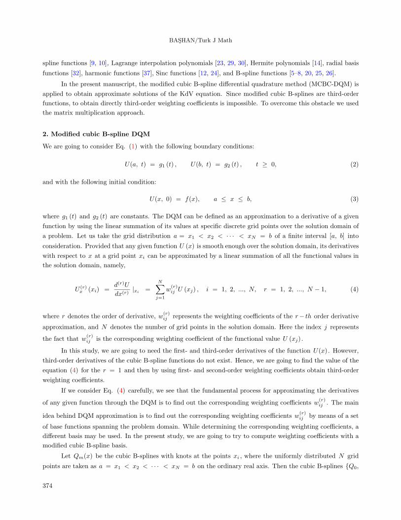
Table 3. Comparison of L2 and L∞ error norms at time t=3.0.

MCBC-DQM (Present) Cubic-DQM [22] Quartic-DQM[22]

ε µ × 104 N ∆t L2 × 106 L∞ × 105 L2 × 106 L∞ × 105 L2 × 106 L∞ × 105

1 4.84 81 10−6 2698.1 771.3 4560 854 2600 704

1 4.84 101 10−6 972.6 268.0 3320 544 1700 434

1 4.84 151 10−6 187.6 53.1 2010 382 850 328

1 4.84 201 10−6 45.8 12.8 - - - -

1 4.84 301 10−6 24.3 6.3 - - - -

Table 4. Invariants for single soliton: ∆t = 0.0005 and N = 201.

t I1 × 101 I2 × 102 I3 × 102 I1 I2 I3

0.0 1.44598000 8.67592500 4.68506900 - - -

1.0 1.44598000 8.67592400 4.68506800 0.0 × 10−9 -1.1 × 10−7 -2.1 × 10−7

2.0 1.44597900 8.67592500 4.68506600 -6.9 × 10−7 0.0 × 10−9 -6.4 × 10−7

3.0 1.44598100 8.67592600 4.68507000 6.9 × 10−7 1.1 × 10−7 2.1 × 10−7

results are in good agreement with those given in earlier works. To show the difference between the cubic-DQM

and MCBC-DQM a comparison of results with the same parameters is given in Table 3. It is obviously seen

from Table 3 that the present results are better than those of the cubic-DQM [22]. As it is straightforwardly

seen from Table 4, the absolute maximum relative changes of invariants are less than 7.0 × 10−7, 1.2 ×10−7, and 6.5 × 10−7 , respectively, during all simulations. We may say that the three invariants computed

are satisfactorily constant.

4.2. Double solitons

Our second test problem has the initial condition given in [15]

U(x, 0) = 3c1 sech2 (A1x + D1) + 3c2 sech

2 (A2x + D2) , (24)

and boundary conditions

U(0, t) = U(2, t) = 0, (25)

where ε = 1, µ = 4.84 × 10−4 , C1 = 0.3, C2 = 0.1, D1 = D2 = −6, ∆t = 0.0005 and N = 201 will

be considered in all simulations.

As seen noticeably in Figure 3 the greater soliton, which has 0.9 amplitude, is located at the left of

the smaller soliton initially. By the time the faster soliton has caught the slower one and at the end of the

simulation the double solitons have a reverse situation. The invariants I1 , I2 and I3 are recorded and reported

with relative changes in invariants in Table 5 for the present case. It is noticeably seen from Table 8 that the

maximum absolute values of relative changes in invariants are less than 2.6 × 10−5 , 5.6 × 10−6 and 2.1 ×10−5 , respectively, during the simulation and therefore they can be considered almost constant.

381

BASHAN/Turk J Math

Figure 3. Simulations for double solitons.

4.3. Triple solitons

Our third test problem is reproduction of three solitons from a single solitary wave initial condition is given by

[16]

U (x, 0) =2

3sech2

(x − 1√108µ

)

with values of ε = 1, µ = 0.0001, ∆t = 0.0001, and N = 751.

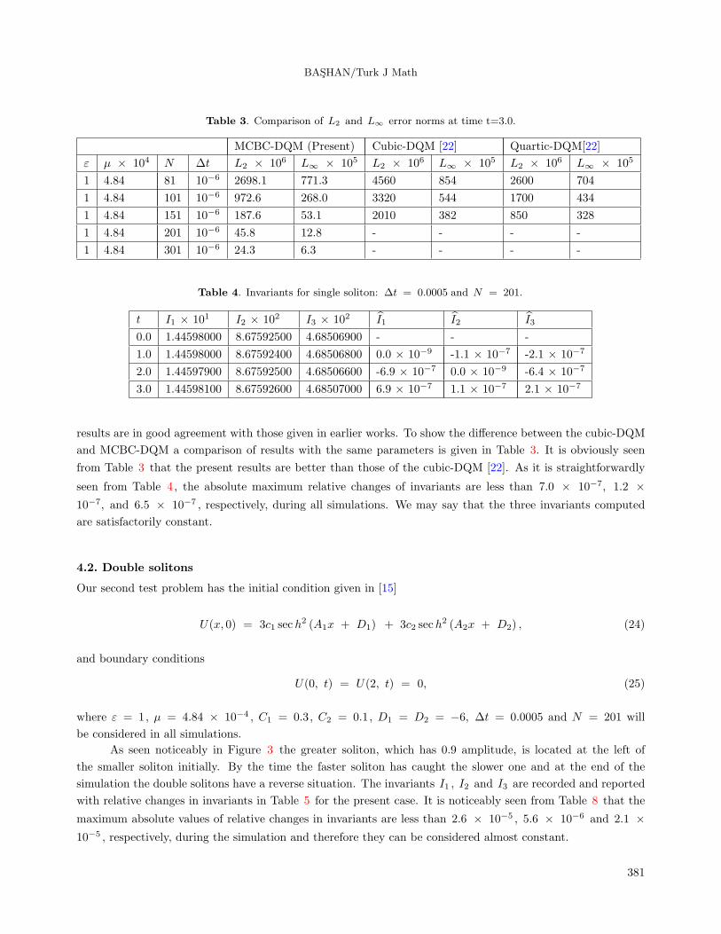
The simulation is run up to time t = 4 in the region [0, 3] . Reproduction of triple waves from single

solitary waves is shown in Figure 4. The three lowest invariants are computed and reported with comparison

of some earlier works given in Table 6. Relative changes in invariants are also added to Table 6. It is seen

noticeably from Table 6 that maximum absolute values of relative changes in invariants are less than 7.3 ×10−7 , 2.6 × 10−6 , and 9.9 × 10−6 , respectively, during the simulation and therefore they can be considered

almost constant again.

382

BASHAN/Turk J Math

Table 5. Invariants for double solitons: ∆t = 0.0005 and N = 201.

Method time I1 I2 I3 I1 I2 I3

Present 0.00 0.228082 0.107062 0.053317 - - -

0.75 0.228078 0.107062 0.053316 -1.4 × 10−5 -4.6 × 10−6 -2.1 × 10−5

1.50 0.228076 0.107062 0.053316 -2.5 × 10−5 -1.8 × 10−6 -1.4 × 10−5

3.00 0.228081 0.107063 0.053317 -8.7 × 10−7 5.6 × 10−6 3.0 × 10−6

MQ [15] 0.00 0.228080 0.107061 0.053318

0.75 0.228016 0.107055 0.053524

1.50 0.228032 0.107057 0.053453

3.00 0.227968 0.107061 0.053265

G [15] 0.00 0.228081 0.107062 0.053316

0.75 0.228135 0.107058 0.053312

1.50 0.228065 0.107059 0.053313

3.00 0.227734 0.107061 0.053316

IMQ [15] 0.00 0.228081 0.107062 0.053316

0.75 0.228964 0.107068 0.053307

1.50 0.228917 0.107072 0.053308

3.00 0.227399 0.107087 0.053307

IQ [15] 0.00 0.228081 0.107062 0.053316

0.75 0.228456 0.107060 0.053312

1.50 0.228386 0.107063 0.053314

3.00 0.227576 0.107069 0.053317

TPS [15] 0.00 0.228079 0.107062 0.053317

0.75 0.227689 0.107056 0.053468

1.50 0.227633 0.107059 0.053410

3.00 0.228071 0.107058 0.053274

4.4. Maxwellian initial condition

For the fourth test problem we have selected the Maxwellian initial condition given by [18]

U (x, 0) = exp(−x2

)with boundary conditions U (−15, t) = U (15, t) = 0 to observe propagation of a single solitary wave.

With the value of µ , the solutions will change. The critical value of µ was given as µc = 0.0625 in [11].

We have investigated solutions of the Maxwellian initial condition for µ = 0.0625, ∆t = 0.001, and N = 481

and we fix the value of ε = 1 to all solutions.

All of the simulations are run up to time t = 10 and shown in Figure 5. When the critical value of µ is

used in simulations as µc = 0.0625 the single solitary wave is observed with no oscillatory tail. This is the result

of balance between the nonlinear and dispersive effects [11]. By decreasing the value of µ to µ = 0.04 with

383

BASHAN/Turk J Math

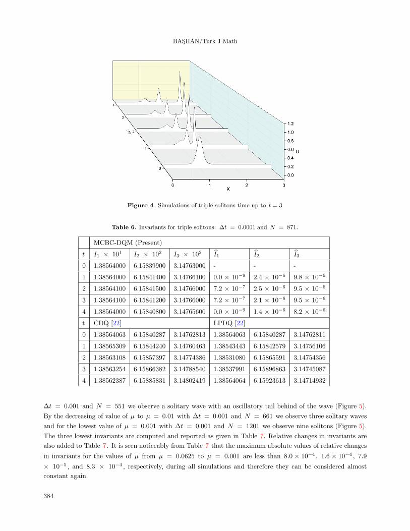
Figure 4. Simulations of triple solitons time up to t = 3

Table 6. Invariants for triple solitons: ∆t = 0.0001 and N = 871.

MCBC-DQM (Present)

t I1 × 101 I2 × 102 I3 × 102 I1 I2 I3

0 1.38564000 6.15839900 3.14763000 - - -

1 1.38564000 6.15841400 3.14766100 0.0 × 10−9 2.4 × 10−6 9.8 × 10−6

2 1.38564100 6.15841500 3.14766000 7.2 × 10−7 2.5 × 10−6 9.5 × 10−6

3 1.38564100 6.15841200 3.14766000 7.2 × 10−7 2.1 × 10−6 9.5 × 10−6

4 1.38564000 6.15840800 3.14765600 0.0 × 10−9 1.4 × 10−6 8.2 × 10−6

t CDQ [22] LPDQ [22]

0 1.38564063 6.15840287 3.14762813 1.38564063 6.15840287 3.14762811

1 1.38565309 6.15844240 3.14760463 1.38543443 6.15842579 3.14756106

2 1.38563108 6.15857397 3.14774386 1.38531080 6.15865591 3.14754356

3 1.38563254 6.15866382 3.14788540 1.38537991 6.15896863 3.14745087

4 1.38562387 6.15885831 3.14802419 1.38564064 6.15923613 3.14714932

∆t = 0.001 and N = 551 we observe a solitary wave with an oscillatory tail behind of the wave (Figure 5).

By the decreasing of value of µ to µ = 0.01 with ∆t = 0.001 and N = 661 we observe three solitary waves

and for the lowest value of µ = 0.001 with ∆t = 0.001 and N = 1201 we observe nine solitons (Figure 5).

The three lowest invariants are computed and reported as given in Table 7. Relative changes in invariants are

also added to Table 7. It is seen noticeably from Table 7 that the maximum absolute values of relative changes

in invariants for the values of µ from µ = 0.0625 to µ = 0.001 are less than 8.0 × 10−4 , 1.6 × 10−4 , 7.9

× 10−5 , and 8.3 × 10−4 , respectively, during all simulations and therefore they can be considered almost

constant again.

384

BASHAN/Turk J Math

Figure 5. Simulations for Maxwellian initial condition.

Figure 6. Simulations of train of ten solitons time up to t = 800.

385

BASHAN/Turk J Math

Table 7. Invariants for Maxwellian initial condition.

µ Time I1 I2 I3 × 101 I1 I2 I3

0.0625 0 1.772454 1.253314 7.883310 - - -

2 1.772455 1.253314 7.883322 5.6 × 10−7 0.0 × 10−9 1.5 × 10−6

4 1.772972 1.253310 7.883376 2.9 × 10−4 -3.1 × 10−6 8.3 × 10−6

6 1.772925 1.253329 7.883488 2.6 × 10−4 1.1 × 10−5 2.2 × 10−5

8 1.773667 1.253245 7.883575 6.8 × 10−4 -5.5 × 10−5 3.3 × 10−5

10 1.771050 1.253196 7.883694 -7.9 × 10−4 -9.4 × 10−5 4.8 × 10−5

0.04 0 1.772454 1.253314 8.729294 - - -

2 1.772460 1.253315 8.729322 3.3 × 10−6 7.9 × 10−7 3.2 × 10−6

4 1.772377 1.253314 8.729339 -4.3 × 10−5 0.0 × 10−9 5.1 × 10−6

6 1.772443 1.253315 8.729348 -6.2 × 10−6 7.9 × 10−7 6.1 × 10−6

8 1.772185 1.253315 8.729380 -1.5 × 10−4 7.9 × 10−7 9.8 × 10−6

10 1.772307 1.253325 8.729328 -8.2 × 10−5 8.7 × 10−6 3.8 × 10−6

0.01 0 1.772453 1.253314 9.857275 - - -

2 1.772453 1.253323 9.857627 0.0 × 10−9 7.1 × 10−6 3.5 × 10−5

4 1.772453 1.253331 9.857994 0.0 × 10−9 1.3 × 10−5 7.2 × 10−5

6 1.772451 1.253332 9.858038 -1.1 × 10−6 1.4 × 10−5 7.7 × 10−5

8 1.772451 1.253332 9.858042 -1.1 × 10−6 1.4 × 10−5 7.7 × 10−5

10 1.772443 1.253332 9.858044 -5.6 × 10−6 1.4 × 10−5 7.8 × 10−5

I1 I2 I3

0.001 0 1.772454 1.253314 1.019567 - - -

2 1.772452 1.253399 1.019973 -1.1 × 10−6 6.7 × 10−5 3.9 × 10−4

4 1.772437 1.253493 1.020409 -9.5 × 10−6 1.4 × 10−4 8.2 × 10−4

6 1.772429 1.253503 1.020408 -1.4 × 10−5 1.5 × 10−4 8.2 × 10−4

8 1.772435 1.253510 1.020383 -1.0 × 10−5 1.5 × 10−4 8.0 × 10−4

10 1.772494 1.253513 1.020388 2.2 × 10−5 1.5 × 10−4 8.0 × 10−4

4.5. Train of solitons

Our fifth and the last test problem has the initial condition given by [19]

U(x, 0) = 0.5

[1 − tanh

|x| − x0

d

], (26)

and boundary conditions

U(−50, t) = U(150, t) = 0, (27)

where −50 ≤ x ≤ 150, d = 5, and x0 = 25 will be considered in all simulations.

The solution vector after a very long run time t = 800 with ε = 0.2, µ = 0.1, ∆t = 0.02, and ∆x

= 0.2 has been shown in Figure 6. A train of 10 solitons has been formed at the end of the simulation. The

invariants I1 , I2 , and I3 are recorded and reported with relative changes in invariants in Table 8 for the present

case. It is noticeably seen from Table 8 that the maximum absolute values of relative changes in invariants are

less than 9.2 × 10−6 , 4.5 × 10−6, and 1.8 × 10−5 , respectively, during this very long run and therefore they

can be considered almost constant.

386

BASHAN/Turk J Math

Table 8. Invariants for train of solitons: ∆t = 0.02 and ∆x = 0.2.

MCBC-DQM (Present) CDQ [22]

t I1 I2 I3 I1 I2 I3 I1 I2 I3

0 50.00011 45.00043 42.30065 - - - 50.00010 45.00045 42.30068

200 50.00042 45.00053 42.30111 6.1 × 10−6 2.2 × 10−6 1.0 × 10−5 49.99671 45.00095 42.30104

400 49.99988 45.00053 42.30135 -4.5 × 10−6 2.2 × 10−6 1.6 × 10−5 50.01744 45.00457 42.30368

600 49.99966 45.00063 42.30138 -8.9 × 10−6 4.4 × 10−6 1.7 × 10−5 50.00556 45.00313 42.30273

800 50.00057 45.00059 42.30137 9.1 × 10−6 3.5 × 10−6 1.7 × 10−5 49.94377 45.01907 42.31425

t FEM [4] FEM [40] FEM [41]

0 50.00 45.000 42.301 50.00021 45.00055 42.30074 50.00000 45.00041 42.30065

200 50.01 45.014 42.110 50.00058 44.99962 42.30098 49.99166 45.00441 42.30647

400 50.00 45.028 42.033 50.00237 44.99921 42.30135 50.06452 45.00995 42.31197

600 49.98 45.042 42.049 49.97857 44.99820 42.29995 50.15105 45.01577 42.31489

800 50.02 45.056 42.064 49.96331 44.99803 42.29974 49.97169 45.02899 42.32111

4.6. Stability analysis

A matrix stability analysis is also investigated for the MCBC-DQM. We have used MATLAB to obtain the

eigenvalues of the coefficient matrix for all of the test problems. Eigenvalues of the suggested method for N

= 201, N = 301, N = 401, and N = 501 number of grids are presented in Figure 7− 11. The maximum

absolute values of eigenvalues for all of the test problems at various numbers of grid points are also tabulated

in Table 9. The eigenvalues have real and imaginary parts for all numbers of grid points. As the numbers of

grid points increase, eigenvalues get greater. This means that to get into the stability region time increments

must be decreased. All the eigenvalues are consistent with the stability criteria [21].

Table 9. Maximum absolute value of eigenvalues at various numbers of grid points.

Grid Number 201 301 401 501

Single Max| Re (λ) | 5.0620 × 103 1.7084 × 104 4.0496 × 104 7.9094 × 104

Max| Im (λ) | 1.5462 × 104 5.2275 × 104 1.2399 × 105 2.4223 × 105

Double Max| Re (λ) | 5.0620 × 103 1.7084 × 104 4.0441 × 104 7.9025 × 104

Max| Im (λ) | 1.5454 × 104 5.2262 × 104 1.2397 × 105 2.4220 × 105

Triple Max| Re (λ) | 1.0459 × 103 3.5298 × 103 4.0496 × 104 7.9094 × 104

Max| Im (λ) | 3.2013 × 103 1.0810 × 104 8.3670 × 103 1.6342 × 104

Maxw. Max| Re (λ) | 6.5367 × 105 2.2061 × 106 5.2294 × 106 1.0214 × 107

Max| Im (λ) | 2.0014 × 106 6.7575 × 106 1.6020 × 107 3.1291 × 107

Train Max| Re (λ) | 1.0459 × 106 3.5298 × 106 8.3670 × 106 1.6342 × 107

Max| Im (λ) | 3.2023 × 106 1.0812 × 107 2.5632 × 107 5.0065 × 107

387

BASHAN/Turk J Math

Figure 7. Eigenvalues for single soliton.

388

BASHAN/Turk J Math

Figure 8. Eigenvalues for double solitons.

389

BASHAN/Turk J Math

Figure 9. Eigenvalues for triple solitons.

390

BASHAN/Turk J Math

Figure 10. Eigenvalues for Maxwellian initial condition.

391

BASHAN/Turk J Math

Figure 11. Eigenvalues for train of solitons.

392

BASHAN/Turk J Math

5. Conclusion

In this work, we have implemented DQM based on modified cubic B-splines for numerical approximation of

KdV equation. Five different test problems have been solved. The performance and accuracy of the present

method have been shown by calculating and comparing the L2 and L∞ error norms with earlier works . As

it seen at Table 2, the present results are acceptable good when compared with some earlier works. As it

seen at Table 3, the present results are better than cubic-DQM[22]. Three lowest invariants are calculated and

reported for all of the test problems. The obtained invariants are acceptable good when compared with some

earlier works. Stability analysis have been done for all of the test problems and all of the eigenvalues are in

convenience with stability criteria [21]. So, MCBC-DQM may be useful to get the numerical solutions of other

important nonlinear problems.

References

[1] Ablowitz MJ, Clarkson PA. Solitons, Nonlinear Evolution Equations and Inverse Scattering. New York, NY, USA:

Cambridge, 1991.

[2] Ablowitz MJ, Segur H. Solitons and Inverse Scattering Transform. Philadelphia, PA, USA: Siam, 1981.

[3] Alexander ME, Morris JL. Galerkin methods for some models equations for nonlinear dispersive waves. J Comput

Phys 1979; 30: 428-451.

[4] Ali AHA, Gardner LRT, Gardner GA. Numerical study of the KdVB equation using B-spline finite elements. J

Math Phys Sci 1993; 27: 37-53.

[5] Bashan A. Numerical solutions of some partial differential equations with B-spline differential quadrature method.

PhD, Inonu University, Malatya, Turkey, 2015.

[6] Bashan A, Karakoc SBG, Geyikli T. Approximation of the KdVB equation by the quintic B-spline differential

quadrature method. Kuwait J Sci 2015; 42: 67-92.

[7] Bashan A, Karakoc SBG, Geyikli T. B-spline Differential Quadrature Method for the Modified Burgers’ Equation.

CUJSE 2015; 12: 001-013.

[8] Bashan A, Ucar Y, Yagmurlu NM, Esen A. Numerical solution of the complex modified Korteweg-de Vries equation

by DQM. Journal of Physics: Conference Series 2016; doi:10.1088/1742-6596/766/1/012028.

[9] Bellman R. Differential quadrature: a technique for the rapid solution of nonlinear differential equations. Journal

of Computational Physics 1972; 40-52.

[10] Bellman R, Kashef B, Lee ES, Vasudevan R. Differential Quadrature and Splines. Computers and Mathematics

with Applications 1976; 371-376.

[11] Berezin YuA, Karpman VA. Nonlinear evolution of disturbances in plasmas and other dispersive media. Sov Phys

JETP 1967; 24: 1049-1056.

[12] Bonzani I. Solution of non-linear evolution problems by parallelized collocation-interpolation methods. Computers

& Mathematics and Applications 1997; 34: 71-79.

[13] Bullough R, Caudrey P. Solitons vol 17 in ”Topics in Current Physics”. Berlin, Germany: Springer, 1980.

[14] Cheng J, Wang B, Du S. A theoretical analysis of piezoelectric/composite laminate with larger-amplitude deflection

effect, Part II: hermite differential quadrature method and application. International Journal of Solids and Structures

2005; 42: 6181-6201.

[15] Dag I, Dereli Y. Numerical solutions of KdV equation using radial basis functions. Appl Math Model 2008; 32:

535-546.

[16] Debussche A, Printems J. Numerical simulation of the stochastic Korteweg-de Vries equation. Physica D 1999; 134:

200-226.

[17] Drazin PG, Johnson RS. Solitons: an Introduction. New York, NY, USA: Cambridge, 1996.

393

BASHAN/Turk J Math

[18] Gardner GA, Ali AHA, Gardner LRT. Simulations of solitons using quadratic spline shape functions. UCNW Maths

1989; 89.03.

[19] Gardner LRT, Gardner GA, Ali AHA. A finite element solution for the Korteweg-de Vries equation using cubic

B-splines. UCNW Maths 1989; 89.01.

[20] Karakoc SBG, Bashan A, Geyikli T. Two different methods for numerical solution of the modified Burgers’ equation.

The Scientific World Journal 2014; http://dx.doi.org/10.1155/2014/780269.

[21] Ketcheson DI. Highly efficient strong stability preserving Runge-Kutta methods with low-storage implementations.

Siam J Sci Comput 2008; 30: 2113-2136.

[22] Korkmaz A. Numerical solutions of some one dimensional partial differential equations using B-spline differential

quadrature methods. PhD, Eskisehir Osmangazi University, Eskisehir, Turkey, 2010.

[23] Korkmaz A. Numerical algorithms for solutions of Korteweg-de Vries equation. Numer Methods Partial Differential

Eq 2010; 26: 1504-1521.

[24] Korkmaz A, Dag I. Shock wave simulations using Sinc Differential Quadrature Method. International Journal for

Computer-Aided Engineering and Software 2011; 28: 654-674.

[25] Korkmaz A, Dag I. Cubic B-spline differential quadrature methods for the advection-diffusion equation. International

Journal of Numerical Methods for Heat & Fluid Flow 2012; 22: 1021-1036.

[26] Korkmaz A, Dag I. Numerical simulations of boundary-forced RLW equation with cubic B-spline-based differential

quadrature methods. Arab J Sci Eng 2013; 38: 1151-1160.

[27] Mittal RC, Jain RK. Numerical solutions of nonlinear Burgers’ equation with modified cubic B-splines collocation

method. Appl Math Comp 2012; 218: 7839-7855.

[28] Prenter PM. Splines and Variational Methods. New York, NY, USA: John Wiley & Sons, 1975.

[29] Quan JR, Chang CT. New sightings in involving distributed system equations by the quadrature methods-I. Comput

Chem Eng 1989; 13: 779-788.

[30] Quan JR, Chang CT. New sightings in involving distributed system equations by the quadrature methods-II.

Comput Chem Eng 1989; 13: 1017-1024.

[31] Sanz Serna JM, Christie I. Petrov-Galerkin methods for nonlinear dispersive waves. J Comput Phys 1981; 39:

94-102.

[32] Shu C, Wu YL. Integrated radial basis functions-based differential quadrature method and its performance. Int J

Numer Meth Fluids 2007; 53: 969-984.

[33] Shu C. Differential Quadrature and Its Application in Engineering. London, UK: Springer-Verlag, 2000.

[34] Soliman AA. Collocation solution of the Korteweg-de Vries equation using septic splines. Int J Comput Maths 2004;

81: 325-331.

[35] Soliman AA, Ali AHA, Raslan KR. Numerical solution for the KdV equation based on similarity reductions. Applied

Mathematical Modelling 2009; 33: 1107-1115.

[36] Spiteri JR, Ruuth SJ. A new class of optimal high-order strong stability-preserving time-stepping schemes. Siam J

Numer Anal 2002; 40: 469-491.

[37] Striz AG, Wang X, Bert CW. Harmonic differential quadrature method and applications to analysis of structural

components. Acta Mechanica 1995; 111: 85-94.

[38] Taha TR, Ablowitz MJ. Analytical and numerical aspects of certain nonlinear evolution equations III. Numerical,

Korteweg-de Vries equation. J Comput Phys 1984; 55: 231-253.

[39] Zabusky NJ. A synergetic approach to problem of nonlinear dispersive wave propagation and interaction. Ames W,

editor. Proceedings Symposium on nonlinear partial differential equations. Academic Press, New York, NY, USA,

1967; pp. 223-258.

[40] Zaki SI. A quintic B-spline finite elements scheme for the KdVB equation. Comput Meth Appl Mech Engrg 2000;

188: 121-134.

[41] Zaki SI. Solitary waves of the Korteweg-de Vries-Burgers’ equation. Comput Phys Commun 2000; 126: 207-218.

394