an autoregressive integrated moving average (arima) model for ghana’s inflation
DESCRIPTION
ÂTRANSCRIPT
Mathematical Theory and Modeling www.iiste.org
ISSN 2224-5804 (Paper) ISSN 2225-0522 (Online)
Vol.3, No.3, 2013
10
An Autoregressive Integrated Moving Average (ARIMA) Model For
Ghana’s Inflation (1985 – 2011).
Buckman Akuffo1*
and Enock Mintah Ampaw2
1. School of Applied Science and Technology, P. O. Box KF 981, Koforidua - Koforidua Polytechnic, Ghana.
2. Department of Applied Mathematics, SAST, P. O. Box KF 981, Koforidua- Koforidua Polytechnic Ghana.
* E-mail of the corresponding author: [email protected]
Abstract
Inflation analysis is indispensable in a developing country like Ghana, which is struggling to achieve the Millennium
Development goals. A literature gap exists in appropriate statistical model on economic variables in Ghana, thus
motivating the authors to come up with a model that could be used to forecast inflation in Ghana. This paper presents
a model of Ghana’s monthly inflation from January 1985 to December 2011 and use the model to forecast twelve
(12) months inflation for Ghana. Using the Box – Jenkins (1976) framework, the autoregressive integrated moving
average (ARIMA) was employed to fit a best model of ARIMA. The seasonal ARIMA model, SARIMA (1, 1, 2) (1,
0, 1) was chosen as the best fitting from the ARIMA family of models with least Akaike Information Criteria (AIC)
of 1156.08 and Bayesian Information Criteria (BIC) of 1178.52. The selected model was used to forecast monthly
inflation for Ghana for twelve (12) months.
Keywords: Inflation, time series, autoregressive, moving average, differencing
1. Introduction
Inflationary analysis or modeling is one of the most important research areas in monetary planning. This is due to the
fact that a high and sustained economic growth in conjunction with low inflation is the central objective of
macroeconomic policy. Achieving and maintaining price stability will be more efficient and effective if the causes of
inflation and the dynamics of its evolution are well understood. It is a fact that monetary policy-makers and planners
worldwide are more interested in stabilizing or reducing inflation through monetary policies (price stability).
Inflation is usually defined as a sustained rise in a broadly based index of commodity prices over some period of
time, (Bomberger and Makinen, 1979). Major components of this definition are that the rise in prices takes place in a
variety of sectors dealing with goods and services; also this increase spans from a rather lengthy period of time rather
than two or more quarters. This means that when the price increases, each unit of currency buys fewer goods and
services and as a result, inflation is an erosion of the purchasing power, which results in loss in real value in the
medium and unit of account in the economy (Stokes, 2009).
Inflation dynamics and evolution can be studied using a stochastic modeling approach that captures the time
dependent structure embedded in time series inflation as a stochastic process. Autoregressive Integrative Moving
Average (ARIMA) models can be applied to describe the component structure of statistical time series especially to
financial/economic time series that show seasonal behaviour, random changes and trends (non-stationary) time
series. Unfortunately, the management of inflation in Ghana over the years has been ineffective. High inflation has
rendered the cost of loanable funds prohibitive. Subsequent high interest rates have in turn prevented productive
sectors of the economy from accessing finance for growth and development (FIAS, 2002). Additionally, in a recent
study by Catoa and Terrones (2003), Ghana was cited as one of the top 25 countries in the world with high inflation
levels. In most cases, economic theories were employed to analyze Ghana’s inflationary experience. A more
vigorous statistical analysis would be more informative and precise. The question that comes up here therefore is
“what is the best time series model and structural form of Ghana’s inflationary experience?” This paper among
others seeks to answer the following research questions:
What is the trend of Ghana’s inflation (1985 – 2011)?
What is the structural form of Ghana’s inflation?
What type of Time Series model can best be used to forecast Ghana’s inflation?
What is the estimated inflation in the next twelve (12) months?
As a matter of fact, Ghana’s inflation experience since independence has been one with a difficulty that policy
makers have being fighting with till today but with little success. From 1957 through 1962, inflation was relative
stable in Ghana and in the neighborhood of the much desired single digit bracket. After 1962, there was
Mathematical Theory and Modeling www.iiste.org
ISSN 2224-5804 (Paper) ISSN 2225-0522 (Online)
Vol.3, No.3, 2013
11
unprecedented macroeconomic instability and very high inflation particularly in the 1970s and early 1980s. For some
time now, Ghana has not had an occasion of sustained single-digit inflation; indeed, it has recorded annual average
inflation rates in excess of 25% in more than half of those years. It was not until 2007 when the new Patriotic Party
(NPP), the government of the day, declared single digit yearly inflation of around 9.64%. However, in just a period
of three (3) years, this figure had risen to 18.6%. Again in 2010 the National Democratic Congress (NDC),
government in the period declared a single digit yearly inflation of 9.56% with its attending problems. These
developments provide enough grounds to be able to model and forecast or predict inflation more accurately and
reliably.
2. Literature Review
The few available studies on inflation in Ghana were conducted in the early to middle 1990s (Sowa, 1996, 1994;
Sowa and Kwakye, 1991; Chhibber and Shaffik, 1991). Recent studies relating to inflation in Ghana have been
mostly part of multi-country efforts and have been broad and less focused (Catao and Terrones, 2003; Loungani and
Swagel, 2001; Braumann, 2000; Bawumiah and Abradu-Otto, 2003, Ocran 2007). Again, many of these studies have
focused on explaining historical nature of inflation and less on the predictive power of the models that were used.
Bawumiah and Atta-Mensah (2003), using a vector error correction forecasting (VECF) model, concluded that
inflation was a monetary phenomenon in Ghana. The authors did not explore the potential for real factors in price
determination however, in their studies.
Sims (1980) has criticized standard macro-econometric policy models for embodying ‘incredible restrictions’,
particularly in the light of the rational expectations hypothesis. The hypothesis suggests that agents use information
about the economy as a whole to generate expectations, which influence variables such as wages, prices or
consumption. In principle, this would imply that any one sectoral equation could embody variables from the system
as a whole. But standard macro-models use relatively restrictive specifications of sectoral equations. As an
alternative, Sims (1980) called for the use of Vector Autoregressive Models (VARs), now among the most widely-
used tools in academic and central bank macro-econometrics (e.g., for studying the transmission mechanism of
monetary policy.) However, there are substantial difficulties in interpreting and using VARs for policy and
forecasting, arising from omitted variables, omitted structural breaks and relevant lags, omitted non-linearities, and
the use of sometimes doubtful identifying restrictions to give economic interpretations to the variable(s).
Univariate time series modelling techniques are becoming an increasingly popular method of analyzing inflation
(Janine et al., 2004). These techniques include models such as Autoregressive (AR), Moving Average (MA), and
Autoregressive Integrated Moving Average (ARIMA). Aidan et al., (1998) considered autoregressive integrated
moving average (ARIMA) forecasting on South African inflationary data from 1990 to 2000. They concluded that
ARIMA models are theoretically justified and can be surprisingly robust with respect to alternative (multivariate)
modeling approaches. Indeed, Stockton and Glassman (1987) upon finding similar results for the United States
commented that it seems somewhat distressing that a simple ARIMA model of inflation should turn in such a
respectable forecast performance relative to the theoretically based specifications. The Box-Jenkins (1976) approach
in using ARIMA seeks to conduct identification, estimation, diagnostic checking, and forecasting a univariate time
series. ARMA models can be viewed as a special class of linear stochastic difference equations.
3.0 Methodology
3.1 Overview of the methodology
The conceptual framework adopted for this work is the Box – Jenkins forecasting also known as autoregressive
integrated moving average (ARIMA) model. The model outlines a three-stage procedure; model identification,
model fitting or estimation, model verification or diagnostics. It is important that any identified model be subjected
to a number of diagnostic checks (usually based on checking the residuals). If the diagnostic checks indicate
problems with the identified model one should return to the model identification stage. Once a model or selection of
models has been chosen; the stability of the estimated parameters should be tested with respect to time frame chosen.
Mathematical Theory and Modeling www.iiste.org
ISSN 2224-5804 (Paper) ISSN 2225-0522 (Online)
Vol.3, No.3, 2013
12
First of all, statistical properties as well as distribution of all time series will be tested by means of coefficient of
skewness and kurtosis, normal probability plots and Jarque-Bera test of normality, to check presence of typical
stylized facts.
Secondly, time series will then be tested for stationarity both graphically and with formal testing schemes by means
of autocorrelation function, partial autocorrelation function and using KPSS test of unit root. If the original or
differenced series comes out to be non-stationary some appropriate transformations will be made for achieving
stationarity, otherwise we will proceed to next phase.
In third phase, based on Box-Jenkins methodology, an appropriate model(s), which best describes the temporal
dependence in the inflation series, will be identified using Autocorrelation Function (ACF) and Partial
Autocorrelation Function (PACF) and estimated through Ordinary Least Square (OLS) method. Estimated model(s)
will be considered most appropriate if it typically simulates historical behaviour as well as constitute white-noise
innovations (Ferridum, 2007). The former will be tested by ACF and PACF of estimated series while the latter will
be tested by a battery of diagnostic tests based on estimated residuals as well as by over-fitting. The best fitting
model(s) will then undergo various residual and normality tests and only qualifying model(s) will be selected and
reserved for forecasting purpose.
Finally, Forecasting performance of the various types of ARIMA models would be compared by computing statistics
like Akaike Information Criteria (AIC), Schwarz Information Criteria (SIC), Thiele Inequality Coefficient (TIC),
Root Mean Square Error (RMSE), Root Mean Square Percent Error (RMSPE), Mean Absolute Error (MAE). On the
basis of these aforementioned selection and evaluation criteria concluding remarks have been drawn.
3.2 The Evolution of ARIMA Model
As stochastic process, time series models evolve from a simple process to a more sophisticated process depending on
the underlining structure.
3.2.1 Moving Average (MA)
Moving average model can be defined as a type of finite impulse response filter process used to analyze a set of data
points by creating a series of averages of different subsets of the full data set. A moving average process with order
p, some constants p ,,,, 3210 , written as MA (p) can be stated as:
ptpttttt ZZZZZX ...3322110 . (1)
Usually 10 and the process is said to be weakly stationary because the mean is constant and the covariance
does not depend on time, t. The mean and variance of the MA process is then given by
q
k
kZtt XVarandXE0
22)(0 (2)
Since the process is purely a combination of tZ, if the tZ are normal, then it implies that the moving average process
is then normal. Also in the MA process,
pktptptptttt ZZZZZCovXXCov ...,..., 0110 (3)
0
;,...,2,1,0
;0
0
2
kpifk
pkif
pkif
k ki
kp
i iZ
(4)
Is can be seen from the above relation that k does not depend on t and the mean is also a constant. This clearly
shows that the process satisfies second order stationarity for all values of the parameters, i . The autocorrelation
function (ACF) of the qMA process is given by
Mathematical Theory and Modeling www.iiste.org
ISSN 2224-5804 (Paper) ISSN 2225-0522 (Online)
Vol.3, No.3, 2013
13
0
0
,...,3,2,1
01
0
2
0
k
qk
qk
k
k
k
q
i
i
kq
i
kii
(5)
Here the autocorrelation cuts off at lag q, which is a special feature of MA processes, and in particular, the MA (1)
process has an autocorrelation function given by
otherwise
k
k
k
0
1
01
2
1
1
(6)
In order to ensure there is a unique MA process for a given ACF, there is an imposition of the condition of
invertibility. This ensures that when the process is written in series form, the series converges. For the MA (1)
process 1 ttt ZZX , the condition is 1 . For the general MA process, we introduce the backward shift
operator, B we have
jtt
j XXB (7)
The corresponding MA (q) process is given by
tt
q
pt ZBZBBBX ...2
210 (8)
The general condition for invertibility is that all the roots of the equation q (B) = 1 lie outside the unit circle (thus
have modulus less than one). Here we regard B as a complex variable and not as an operator.
3.2.2 Autoregressive (AR)
The autoregressive structure is a stochastic process that assumes that current data can be modeled as a weighted
summation of previous values plus a random term. The process tX is regressed on past values of itself and his
explains the prefix ‘auto’ in the regression process. Assume the random term, tZ is purely random that is the term
with mean zero and standard deviation z . Then the autoregressive process of order p or AR (p) process is given by
tptptttt ZXXXXX ...332211 . (9)
In particular, the first AR process, AR (1) can be stated as ttt ZXX 1 , which is sometimes called the Markov
first order property of the AR. Provided 1 , then the AR (1) may be written as an infinite moving average
process.
In effect 0tXE ACVF is given by

Mathematical Theory and Modeling www.iiste.org
ISSN 2224-5804 (Paper) ISSN 2225-0522 (Online)
Vol.3, No.3, 2013
14
.
12
2
2
0
2
y
k
k
ik
i
i
jkt
i
it
i
ktt ZZEXXEk
(10)
Since k does not depend on time, it can be shown that kk . This implies an AR process of order 1 is a
second-order stationary provided that 1 , and the ACF is then given by ...,3,2,1,0, kk k
In general AR (p) an autoregressive process with order p can be written as
tt
p
p ZX )...1( 3
3
2
21 (11)
or better still
tp
p
t
t ZfZ
X )()...1( 3
3
2
21
. (12)
This gives the AR an infinite series of MA with a mean of zero. Thus there is a link between an MA and AR process.
This can be easily shown by introducing the backward shift operator B, then we have
tt ZX )1( and tt
t ZZ
X ...1)1(
22
. (13)
Conditions needed to ensure that various series converge, and hence that the variance exists, and the auto covariance
can be defined are crucial in modelling autoregressive processes. Essentially these conditions are that the i become
small quickly enough, for large i. The i may not be able to be found. The alternative is to work with the i .The
auto covariance function (ACVF) is expressible in terms of the roots i for, i = 1, 2, 3, ...p of the auxiliary equation
0...1
1
p
pp yy . With the auto covariance function, the process can then be described.
3.2.3 Combination of AR and MA processes
ARMA models are formed by combining both the AR and MA structures to form a stochastic process. A model with
p AR terms and q MA terms is said to be an autoregressive moving average (ARMA) process of order qp, . This
combination is given by
qtqtttptpttt ZZZZXXXX ...... 22112211 (14)
Alternative expressions are possible using the backshift operator B as
tt ZX BB (15)
where
ptptttt XXXXX ...2211B (16a)
and
qtqtttt ZZZZZ ...2211B (16b)
Thus tXB and tZB are polynomials of order p and q respectively such that
p
pBBBB ...1 2
21 (17a)
and
q
qBBBB ...1 2
21 (17b)

Mathematical Theory and Modeling www.iiste.org
ISSN 2224-5804 (Paper) ISSN 2225-0522 (Online)
Vol.3, No.3, 2013
15
It must be noted that an ARMA model can be states as a pure AR or a pure MA process as and when the need arise.
Constraints required on the model parameters to render the processes stationary and invertible are the same as for a
pure AR or a pure MA processes. That is for stability to be guaranteed or to achieve causality, the values of i are
the roots of the polynomial 0B , should lie outside the unit circle. Similarly, the values i , of which
invertibility is guaranteed, are such that the roots of 0B lie outside the unit circle.
The ARMA model formulation is important because, stationary time series mat often be adequately modeled with
fewer parameters as oppose to a pure MA or a pure AR process. Thus the use of ARMA model leads to dealing with
fewer parameters which save time in computation and interpretation yet yields an adequate representation of the data
being studied.
3.2.4 Integrated ARMA (ARIMA) models
Autoregressive moving average (ARMA) models are formed by combining both the autoregressive (AR) and moving
average (MA) structures to form a stochastic process. A model with p AR terms and q MA terms is said to be an
autoregressive moving average (ARMA) process of order qp, .
It should be noted that an ARMA process can be purely AR terms with order p or purely MA process with order
p . In general, most time series are non – stationary. In order to fit and exploit the nice properties of a stationary
model, it is important to remove the non-stationarity sources of variation. This can be done by differencing the series
or taking appropriate transformation such as taking logarithms or root of the data etc (Chinomona, 2009).
For an autoregressive integrated moving average processes (ARIMA) processes, when differenced say d times, the
process is an ARMA process. Assume the differenced process is denoted by Wt. Then Wt is given by
t
d
t
d
t XXW B 1 (18)
Then the general form of the ARIMA model process is given by
qtqtttptpttt WWWW ...... 22112211 This general equation can be transformed in its polynomial for as
tt ZW BB
or
tt
dZX BBB 1
(19)
The model for tW describe the thd order difference of the process tX and is said to be an ARIMA process of order
qdp ,, . Practically, the first order differencing yields adequate results or produces stationarity, and so the value
of d is often set to one (1). For this reason, one often will see ARIMA process of order qp ,1, . In practice, a
random walk can be said to be an ARIMA (0, 1, 0).
It must also be noted that overdifferencing introduces autocorrelation and should be avoided. Box – Jenkins rule of
thumb states that the optimum order of differencing is the one with the smallest standard deviation.
Again, according to Slutsky, (1980) if you pass even a pure white noise through a high band filter, you may still get
peaks called pseudo-peaks, which are not real.
3.2.5 Seasonal ARIMA (SARIMA)
More often than not, practical time series contain a seasonal component which repeats itself periodically, for
instance, every s observation. The notation s denotes the seasonal period. For instance, with 12s in this case we
may expect the series, tx to depend on values at annual lags such as 12tx and 24tx and on more recent non –
seasonal values as 1x and 2x . A seasonal ARIMA model, SARIMA of order s
QDPqdp ,,,, , and D
order of seasonal differences, P order of seasonal AR process, Q order of seasonal MR process, s = the
seasonality may be defined as
Mathematical Theory and Modeling www.iiste.org
ISSN 2224-5804 (Paper) ISSN 2225-0522 (Online)
Vol.3, No.3, 2013
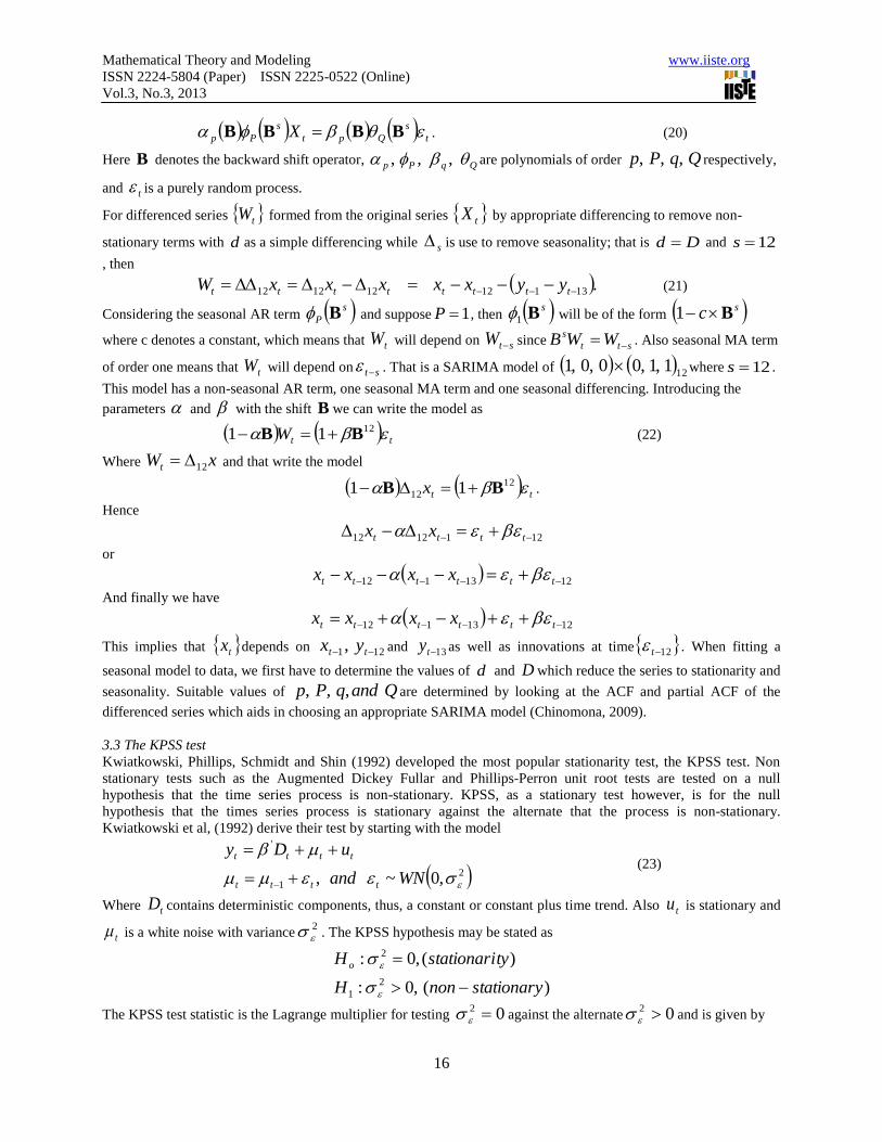
16
t
s
Qpt
s
Pp X BBBB . (20)
Here B denotes the backward shift operator, QqPp ,,, are polynomials of order QqPp ,,, respectively,
and t is a purely random process.
For differenced series tW formed from the original series tX by appropriate differencing to remove non-
stationary terms with d as a simple differencing while s is use to remove seasonality; that is Dd and 12s
, then
.13112121212 tttttttt yyxxxxxW (21)
Considering the seasonal AR term s
P B and suppose 1P , then sB1 will be of the form sc B1
where c denotes a constant, which means that tW will depend on stW since stt
s WWB . Also seasonal MA term
of order one means that tW will depend on st . That is a SARIMA model of 12
1,1,00,0,1 where 12s .
This model has a non-seasonal AR term, one seasonal MA term and one seasonal differencing. Introducing the
parameters and with the shift B we can write the model as
ttW 1211 BB (22)
Where xWt 12 and that write the model
ttx 12
12 11 BB .
Hence
1211212 tttt xx
or
1213112 tttttt xxxx
And finally we have
1213112 tttttt xxxx
This implies that tx depends on 121, tt yx and 13ty as well as innovations at time 12t . When fitting a
seasonal model to data, we first have to determine the values of d and D which reduce the series to stationarity and
seasonality. Suitable values of QandqPp ,,, are determined by looking at the ACF and partial ACF of the
differenced series which aids in choosing an appropriate SARIMA model (Chinomona, 2009).
3.3 The KPSS test
Kwiatkowski, Phillips, Schmidt and Shin (1992) developed the most popular stationarity test, the KPSS test. Non
stationary tests such as the Augmented Dickey Fullar and Phillips-Perron unit root tests are tested on a null
hypothesis that the time series process is non-stationary. KPSS, as a stationary test however, is for the null
hypothesis that the times series process is stationary against the alternate that the process is non-stationary.
Kwiatkowski et al, (1992) derive their test by starting with the model
2
1
'
,0~,
WNand
uDy
tttt
tttt
(23)
Where tD contains deterministic components, thus, a constant or constant plus time trend. Also tu is stationary and
t is a white noise with variance2
. The KPSS hypothesis may be stated as
)(,0:
)(,0:
2
1
2
stationarynonH
tystationariH o
The KPSS test statistic is the Lagrange multiplier for testing 02 against the alternate 02 and is given by

Mathematical Theory and Modeling www.iiste.org
ISSN 2224-5804 (Paper) ISSN 2225-0522 (Online)
Vol.3, No.3, 2013
17
2
1
22
ˆ
ˆ
T
t tSTKPSS (24)
Where
t
j jt uS1
2 ˆˆ and tu is the residual of a regression of ty on tD and 2 is a consistent estimate of the
long-run variance of tu using tu Kwiatkowski et al, (1992). The R software comes with the KPSS with its
associated critical values for interpretation just as other computer software.
4. Results
4.1 The trend of inflation in Ghana
To be able to examine the trend of inflation in Ghana, a time plot of the inflation data has to be examined. The data
and time plots of the data are discussed separately in the next session.
4.1.1 Preliminary Analysis
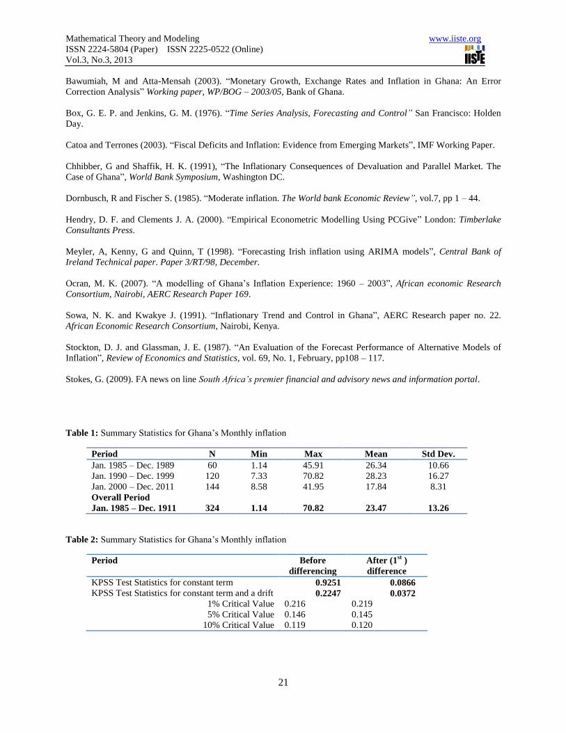
Table 1 shows the summary descriptive statistics of Ghana’s inflation from January 1985 – December 2010. The data
is divided into the various decades within the span of data for the study. From Table 1, it is evident that the period
January 1985 – December 1989 recorded the lowest level of inflation of 1.14 percent (%). Also, the period January
1990 – December 1999 recorded the highest inflation of 70.82%. Again, January 1990 – December 1999 recorded
highest average and standard deviation of 28.23% and 16.27 respectively. This high average and corresponding
standard deviation implies the period was the most volatile.
After this era, however, there was decrease in inflation to an average of 17.84 % with a deviation of 8.31. This
implies the period January 2000 to December 2011 recorded the most stable inflation levels compared to the past two
periods. This can be attributed to the targeting inflation policy pursed during this era (starting 2007) in pursuance of
the Millennium Development Goals (MDGs) and stable democratic governance within the period.
The non constant mean and standard deviation in the data suggest that Ghana’s inflation data may be non-stationary;
this however needs to be verified formally. This means inflation over the period has been very volatile.
4.1.2 Time Plot of Data
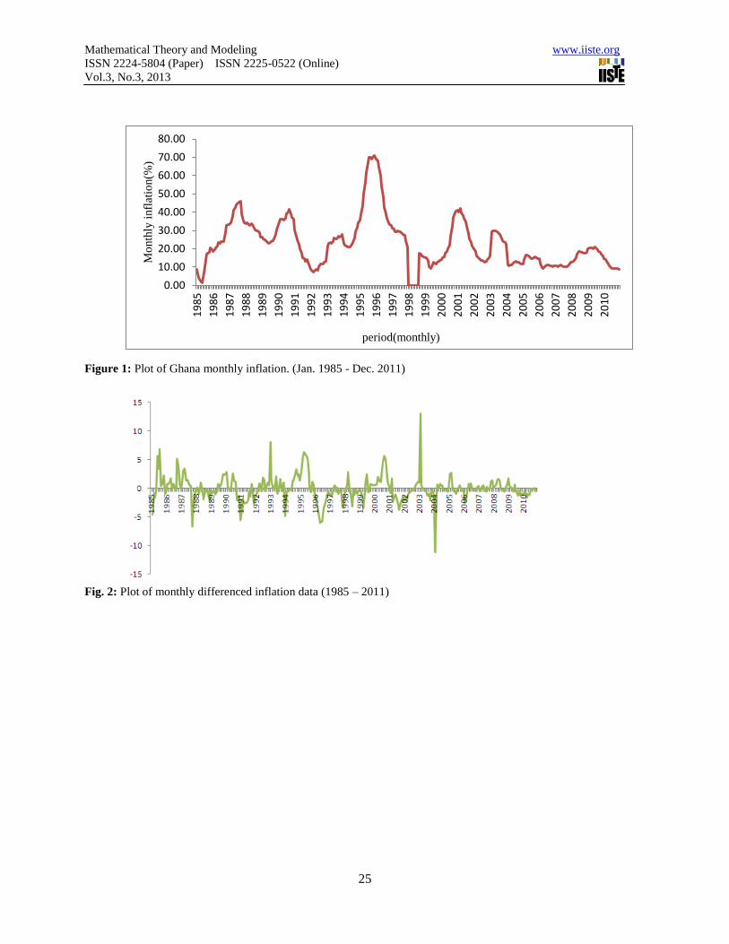
Plots of data actually reveal important features of a time series, such as trend, seasonal variation, outliers and
discontinuities, which can be seen.
From Figure 1, the plots of Ghana inflation do not reveal a clear trend, outlier or discontinuity but a slight seasonal
effect can be noticed. It can be seen that inflation in Ghana was soaring 1986 to the last quarter of 1994 where the
variation peaked; through to the end of 1996. The 2000s began with another moderate inflation episode with a period
average of 25.7% having come from inflationary experience where the three-year period average was 18.7%. Unlike
other countries that did not stay in moderate inflationary experience for long (Dornbusch and Fisher, 1993), Ghana
appears to have been saddled with persistent moderate inflation for far too long.
4.2 The structural form of Ghana’s inflationary data (1985:01 – 2011:12)
Evidence from the data statistics and the time plot suggest that the monthly inflation may not be stationary. To
formally test various variations identified, the KPSS test for stationarity is applied.
4.2.1 Test for Stationarity: KPSS Unit root test
The KPSS test for stationarity was conducted to check for stationarity at levels and the results is as presented in
Table 2. The hypothesis to test for stationarity in using the KPSS is stated as follows:
Mathematical Theory and Modeling www.iiste.org
ISSN 2224-5804 (Paper) ISSN 2225-0522 (Online)
Vol.3, No.3, 2013
18
)(,0:
)(,0:
2
1
2
stationarynonH
tystationariH o
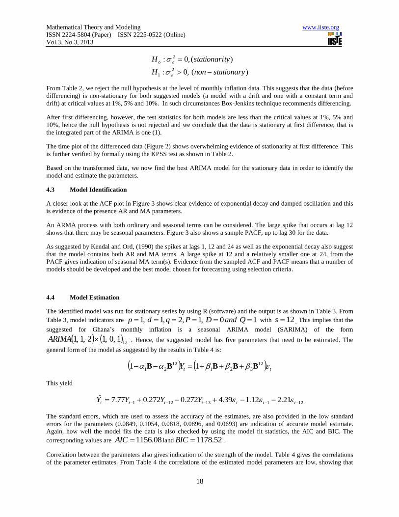
From Table 2, we reject the null hypothesis at the level of monthly inflation data. This suggests that the data (before
differencing) is non-stationary for both suggested models (a model with a drift and one with a constant term and
drift) at critical values at 1%, 5% and 10%. In such circumstances Box-Jenkins technique recommends differencing.
After first differencing, however, the test statistics for both models are less than the critical values at 1%, 5% and
10%, hence the null hypothesis is not rejected and we conclude that the data is stationary at first difference; that is
the integrated part of the ARIMA is one (1).
The time plot of the differenced data (Figure 2) shows overwhelming evidence of stationarity at first difference. This
is further verified by formally using the KPSS test as shown in Table 2.
Based on the transformed data, we now find the best ARIMA model for the stationary data in order to identify the
model and estimate the parameters.
4.3 Model Identification
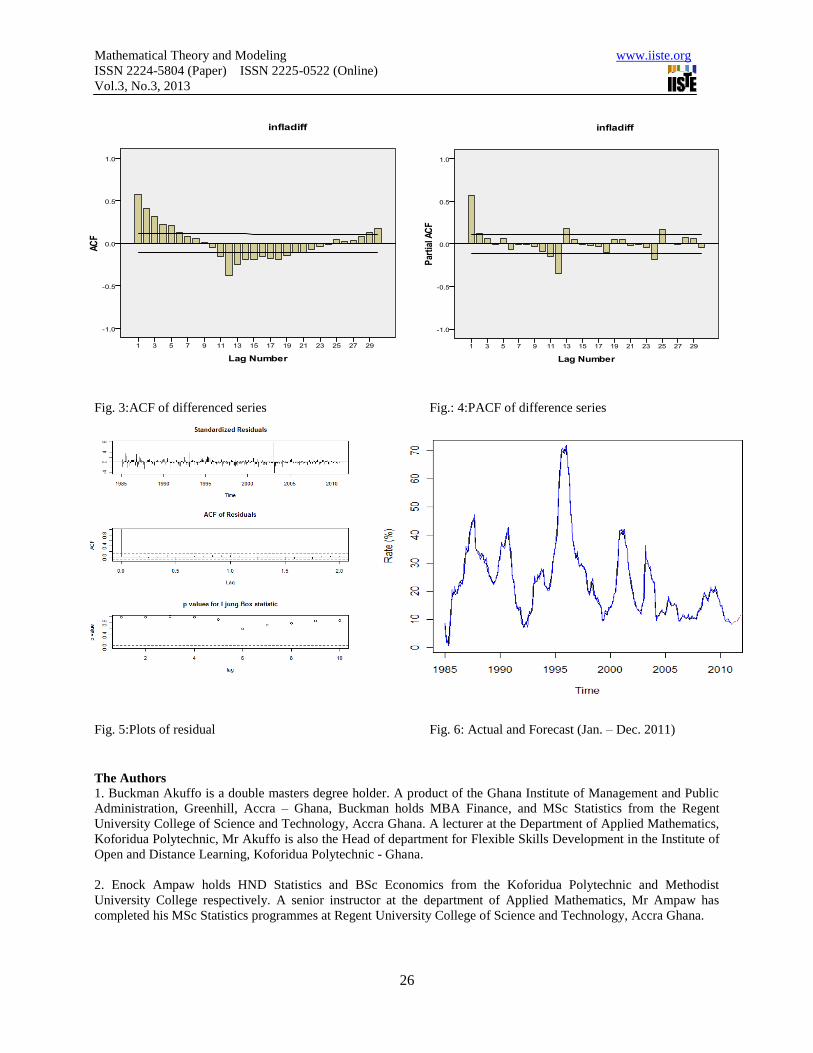
A closer look at the ACF plot in Figure 3 shows clear evidence of exponential decay and damped oscillation and this
is evidence of the presence AR and MA parameters.
An ARMA process with both ordinary and seasonal terms can be considered. The large spike that occurs at lag 12
shows that there may be seasonal parameters. Figure 3 also shows a sample PACF, up to lag 30 for the data.
As suggested by Kendal and Ord, (1990) the spikes at lags 1, 12 and 24 as well as the exponential decay also suggest
that the model contains both AR and MA terms. A large spike at 12 and a relatively smaller one at 24, from the
PACF gives indication of seasonal MA term(s). Evidence from the sampled ACF and PACF means that a number of
models should be developed and the best model chosen for forecasting using selection criteria.
4.4 Model Estimation
The identified model was run for stationary series by using R (software) and the output is as shown in Table 3. From
Table 3, model indicators are 10,1,2,1,1 QandDPqdp with 12s . This implies that the
suggested for Ghana’s monthly inflation is a seasonal ARIMA model (SARIMA) of the form
12
1,0,12,1,1 ARIMA . Hence, the suggested model has five parameters that need to be estimated. The
general form of the model as suggested by the results in Table 4 is:
ttY 12
321
12
21 11 BBBBB
This yield
12113121 21.212.139.4272.0272.077.7ˆ ttttttt YYYY
The standard errors, which are used to assess the accuracy of the estimates, are also provided in the low standard
errors for the parameters (0.0849, 0.1054, 0.0818, 0.0896, and 0.0693) are indication of accurate model estimate.
Again, how well the model fits the data is also checked by using the model fit statistics, the AIC and BIC. The
corresponding values are 08.1156AIC land 52.1178BIC .
Correlation between the parameters also gives indication of the strength of the model. Table 4 gives the correlations
of the parameter estimates. From Table 4 the correlations of the estimated model parameters are low, showing that

Mathematical Theory and Modeling www.iiste.org
ISSN 2224-5804 (Paper) ISSN 2225-0522 (Online)
Vol.3, No.3, 2013
19
they do not explain the same variations in the model. The parameter estimate for the model together with the
corresponding t – values are as presented in Table 5. From Table 5, all the parameters are significant and this also
confirms that the model best fits the data.
In an attempt to find a more parsimonious model (if it does exist), a number of models are run and their outcomes
compared with the model identified above.
The models included )2,1,1(ARIMA , 12
1,0,11,1,1SARIMA and 12
1,0,11,1,2SARIMA . In all
these models, the parameters of the estimated models were found not to be superior to that of the
12
1,0,12,1,1 ARIMA
The corresponding fit statistics for the ARIMA (1, 1, 2) are:
97.1231AIC and 77.1247BIC . Thus the ARIMA (1, 1, 2) has bigger AIC and BIC than the seasonal
12
1,0,12,1,1 ARIMA . It is worth mentioning also that though the ARIMA (1, 1, 2) has fewer parameters,
all the parameters are also not significant.
Another model tested was 12
1,0,11,1,2 ARIMA , which has the same number of parameters as
12
1,0,12,1,1 ARIMA . The Durbin-Watson statistics of 1.047 in the model suggests that
12
1,0,11,1,2 ARIMA exhibits heteroscedasticity. Its fit statistics are 11.1505AIC and
which are all greater than the fit statistics of the seasonal 12
1,0,12,1,1 ARIMA
Another candidate tested was more parsimonious model, a seasonal ARIMA (1, 1, 1) (1, 0, 1)12 with equal number of
AR and MA terms, 12
1,0,11,1,1 ARIMA and fewer parameters than the 12
1,0,12,1,1 ARIMA
which stands out as the best fit model so far.
The ARIMA (1, 1, 1) (1, 0, 1)12 results show that all the estimated parameters are significant with its Durbin-Watson
statistic of approximately 2, which shows evidence of no heteroscedasticity. However, the model fit statistics of AIC
= 1212.05 and BIC = 1385.99 are greater than that of ARIMA (1, 1, 2) (1, 0, 1)12.
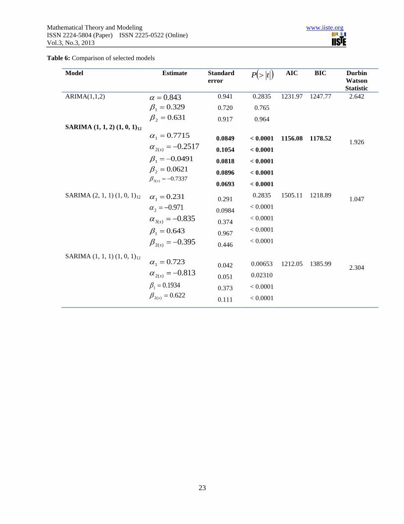
Table 6 shows the estimated models with the corresponding estimates, standard errors, significant probabilities, AIC
and BIC for each parameter.
Considering the significance of the estimated parameters for the various models, the number of parameters estimated
together with the least AIC and BIC fit statistics, it can be established that the best fit model for inflation from 1985
to 2010 in Ghana is the seasonal SARIMA (1, 1, 2) (1, 0, 1) given by
12113121 21.212.139.4272.0272.077.7ˆ ttttttt YYYY
This means holding all factors constant, this month inflation is a linear function of the previous month, the twelfth
month’s inflation, less the thirteenth month’s inflation and some innovation terms.
4.5 Diagnostics check of the identified model: SARIMA (1, 1, 2) (1, 0, 1)12
Residuals from a model that fits the data well should have zero mean, uncorrelated and show uniform random
variability over time, that is, it should be a white noise.
89.1218BIC
Mathematical Theory and Modeling www.iiste.org
ISSN 2224-5804 (Paper) ISSN 2225-0522 (Online)
Vol.3, No.3, 2013
20
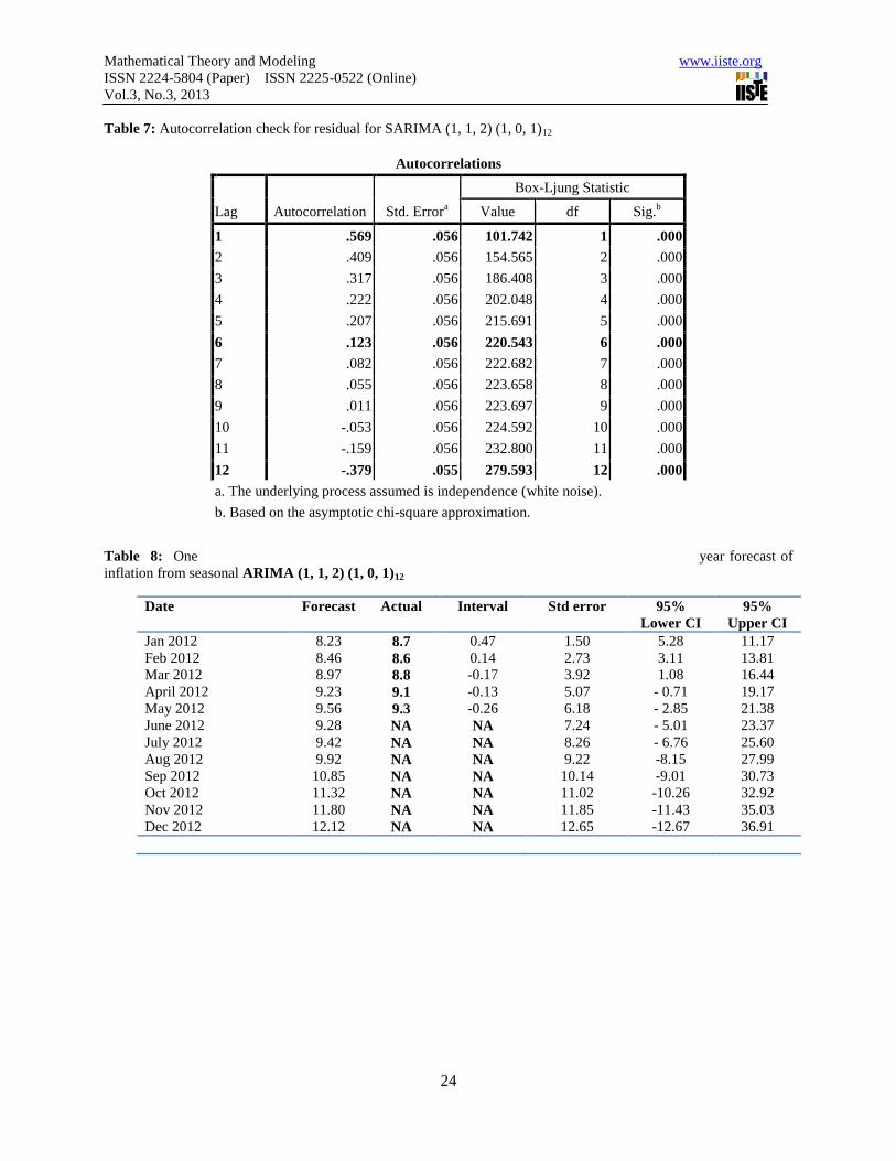
Table 7 shows the autocorrelations at some lags together with Q – statistics for the Box – Ljung test, based on the
asymptotic chi-square approximation. The results show that none of the Q – statistics is statistically significant,
meaning the absence of autocorrelation. The plot of standardized residuals, ACF of the residuals and the p – values
of the Box – Ljung statistics are presented in Figure 4.
The ACF of the residuals immediately die out from lag one (1), which means the residual are white noise. Any
significant autocorrelation gives an indication of misspecification. The pattern of the standard residuals, ACF and the
p – values for the Ljung – Box statistics show overwhelming evidence that the residuals are independent implying
the model fits the data well. Now that a best fit model has been fitted, the next step is to use the identified model
estimated to forecast future values of the series.
4.6 Forecasting
The principal objective of time series modelling and analysis is forecasting. The Holt-Winters forecasting procedure
was applied in forecasting inflation for the next twelve months. The seasonal ARIMA (1, 1, 2) (1, 0, 1)12 was used to
generate the forecast of inflation for the period January 2011 to December 2011. The forecast values, and the
standard deviation as well as a 95% confidence interval are presented in Table 8.
The forecast values are superimposed on the actual data values to aid visual inspection of the series. The output from
the R software is as shown in Figure 5.
From Table 8, the forecast values lie within the limits. Although the model fits the data well, the wider confidence
limit gives an indication of low forecasting power, which may be as a result of the time span of the data used.
5. Conclusion
The study was based on monthly inflation data, and has been used to estimate various possible ARIMA models
according to suggestions from ACF and PACF sequence plots. Among the estimated models, the best model for
inflation forecast for the period 1985:01 – 2011:12 have been obtained. The comparative performance of these
ARIMA models have been checked and verified by using the statistics; AIC, BIC and Durbin – Watson statistics.
The comparison indicated that the best ARIMA model was the seasonal ARIMA (1, 1, 2) (1, 0, 1)12. It has also been
observed that the plots of actual values and the forecasted values of inflation were very close. This means that the
selected model best fit the data and hence, appropriate for forecasting. The forecast error of less than 4% (forecast
error of 3.4%) also gave further evidence that the model selected has very strong predictive power. The proposed
model for Ghana’s inflationary data is
12113121 21.212.139.4272.0272.077.7ˆ ttttttt yyyY
This means holding all factors constant, this month inflation is a linear function of the previous month, the twelfth
month’s inflation, less the thirteenth month’s inflation and random terms from the previous and last twelfth month.
References
Akinboade, O. A, Niedermeier, E. W. and Siebrits, F. K. (2001). “Inflation Dynamics: Implication for Policy”,
Discussion paper, Department of Economics, University of South Africa.
Aaron, J and Muellbauer, J (2008). “Construction of CPIX Data for Forecasting and Modelling in South Africa”
Economic journal of South Africa, vol. 72 no 5, page 884 – 912.
Atta, J. K, Jefferies K. R. and Mannathoko I. (1996). “Small Countries Experience with Exchange Rate and Inflation:
the case of Botswana” Journal of African Economics, vol. 5(2), pp 293 – 326.
Mathematical Theory and Modeling www.iiste.org
ISSN 2224-5804 (Paper) ISSN 2225-0522 (Online)
Vol.3, No.3, 2013
21
Bawumiah, M and Atta-Mensah (2003). “Monetary Growth, Exchange Rates and Inflation in Ghana: An Error
Correction Analysis” Working paper, WP/BOG – 2003/05, Bank of Ghana.
Box, G. E. P. and Jenkins, G. M. (1976). “Time Series Analysis, Forecasting and Control” San Francisco: Holden
Day.
Catoa and Terrones (2003). “Fiscal Deficits and Inflation: Evidence from Emerging Markets”, IMF Working Paper.
Chhibber, G and Shaffik, H. K. (1991), “The Inflationary Consequences of Devaluation and Parallel Market. The
Case of Ghana”, World Bank Symposium, Washington DC.
Dornbusch, R and Fischer S. (1985). “Moderate inflation. The World bank Economic Review”, vol.7, pp 1 – 44.
Hendry, D. F. and Clements J. A. (2000). “Empirical Econometric Modelling Using PCGive” London: Timberlake
Consultants Press.
Meyler, A, Kenny, G and Quinn, T (1998). “Forecasting Irish inflation using ARIMA models”, Central Bank of
Ireland Technical paper. Paper 3/RT/98, December.
Ocran, M. K. (2007). “A modelling of Ghana’s Inflation Experience: 1960 – 2003”, African economic Research
Consortium, Nairobi, AERC Research Paper 169.
Sowa, N. K. and Kwakye J. (1991). “Inflationary Trend and Control in Ghana”, AERC Research paper no. 22.
African Economic Research Consortium, Nairobi, Kenya.
Stockton, D. J. and Glassman, J. E. (1987). “An Evaluation of the Forecast Performance of Alternative Models of
Inflation”, Review of Economics and Statistics, vol. 69, No. 1, February, pp108 – 117.
Stokes, G. (2009). FA news on line South Africa’s premier financial and advisory news and information portal.
Table 1: Summary Statistics for Ghana’s Monthly inflation
Period N Min Max Mean Std Dev.
Jan. 1985 – Dec. 1989
Jan. 1990 – Dec. 1999
Jan. 2000 – Dec. 2011
Overall Period
Jan. 1985 – Dec. 1911
60
120
144
324
1.14
7.33
8.58
1.14
45.91
70.82
41.95
70.82
26.34
28.23
17.84
23.47
10.66
16.27
8.31
13.26
Table 2: Summary Statistics for Ghana’s Monthly inflation
Period Before
differencing
After (1st )
difference
KPSS Test Statistics for constant term
KPSS Test Statistics for constant term and a drift
1% Critical Value
5% Critical Value
10% Critical Value
0.216
0.146
0.119
0.9251
0.2247
0.219
0.145
0.120
0.0866
0.0372

Mathematical Theory and Modeling www.iiste.org
ISSN 2224-5804 (Paper) ISSN 2225-0522 (Online)
Vol.3, No.3, 2013
22
Table 3: Estimated model for inflation: 12
1,0,12,1,1 ARIMA
Call: Arima(x = D, order = c(1, 1, 2), seasonal = list(order = c(1, 0, 1)))
Coefficient
Std error
Sigma^2 estimate
Log Likelihood
Durbin – Watson statics
AIC
BIC
AR1
0.7715
0.0849
2.255
-572.04
1.926
1156.08
1178.52
MA1 -0.2517
0.0818
MA2
-0.0491
0.0818
SAR1
0.0621
0.0896
SMA1
-0.7337
0.0693
Table 4: Correlation of parameter estimates:
12
1,0,12,1,1 ARIMA
Parameter AR(p =1) SAR(P =1) MA(q = 2) SMA(Q=1)
AR(p =1)
SAR(P =1)
MA(q = 2)
SMA(Q=1)
1
2
1
2
3
1
1
0.215
0.124
0.317
0.661
2
1
0.113
0.316
0.222
1
1
0.052
0.311
2
1
0.042
3
1
Table 5: Significance of the parameter estimates for SARIMA :( 1, 1, 2) (1, 0, 1)12
Parameter Estimate Standard error t - value tP
1
2
1
2
3
0.7715
-0.2517
-0.0491
0.0621
-0.7337
0.849
0.1054
0.0818
0.0896
0.0693
0.0628
0.0222
0.1240
0.0920
0.0101
< 0.0001
< 0.0001
< 0.0001
< 0.0001
< 0.0001
Mathematical Theory and Modeling www.iiste.org
ISSN 2224-5804 (Paper) ISSN 2225-0522 (Online)
Vol.3, No.3, 2013
23
Table 6: Comparison of selected models
Model Estimate Standard
error tP AIC BIC Durbin
Watson
Statistic
ARIMA(1,1,2)
SARIMA (1, 1, 2) (1, 0, 1)12
SARIMA (2, 1, 1) (1, 0, 1)12
SARIMA (1, 1, 1) (1, 0, 1)12
843.0
329.01
631.02
7715.01
2517.0)(2 s
0491.01
0621.02
7337.0)(3 s
231.01
971.02
835.0)(3 s
643.01
395.0)(2 s
723.01
813.0)(2 s
1934.01
622.0)(2 s
0.941
0.720
0.917
0.0849
0.1054
0.0818
0.0896
0.0693
0.291
0.0984
0.374
0.967
0.446
0.042
0.051
0.373
0.111
0.2835
0.765
0.964
< 0.0001
< 0.0001
< 0.0001
< 0.0001
< 0.0001
0.2835
< 0.0001
< 0.0001
< 0.0001
< 0.0001
0.00653
0.02310
< 0.0001
< 0.0001
1231.97
1156.08
1505.11
1212.05
1247.77
1178.52
1218.89
1385.99
2.642
1.926
1.047
2.304
Mathematical Theory and Modeling www.iiste.org
ISSN 2224-5804 (Paper) ISSN 2225-0522 (Online)
Vol.3, No.3, 2013
24
Table 7: Autocorrelation check for residual for SARIMA (1, 1, 2) (1, 0, 1)12
Table 8: One year forecast of
inflation from seasonal ARIMA (1, 1, 2) (1, 0, 1)12
Date Forecast Actual Interval Std error 95%
Lower CI
95%
Upper CI
Jan 2012 8.23 8.7 0.47 1.50 5.28 11.17
Feb 2012 8.46 8.6 0.14 2.73 3.11 13.81
Mar 2012 8.97 8.8 -0.17 3.92 1.08 16.44
April 2012 9.23 9.1 -0.13 5.07 - 0.71 19.17
May 2012 9.56 9.3 -0.26 6.18 - 2.85 21.38
June 2012 9.28 NA NA 7.24 - 5.01 23.37
July 2012 9.42 NA NA 8.26 - 6.76 25.60
Aug 2012 9.92 NA NA 9.22 -8.15 27.99
Sep 2012 10.85 NA NA 10.14 -9.01 30.73
Oct 2012 11.32 NA NA 11.02 -10.26 32.92
Nov 2012
Dec 2012
11.80
12.12 NA
NA
NA
NA
11.85
12.65
-11.43
-12.67
35.03
36.91
Autocorrelations
Lag Autocorrelation Std. Errora
Box-Ljung Statistic
Value df Sig.b
1 .569 .056 101.742 1 .000
2 .409 .056 154.565 2 .000
3 .317 .056 186.408 3 .000
4 .222 .056 202.048 4 .000
5 .207 .056 215.691 5 .000
6 .123 .056 220.543 6 .000
7 .082 .056 222.682 7 .000
8 .055 .056 223.658 8 .000
9 .011 .056 223.697 9 .000
10 -.053 .056 224.592 10 .000
11 -.159 .056 232.800 11 .000
12 -.379 .055 279.593 12 .000
a. The underlying process assumed is independence (white noise).
b. Based on the asymptotic chi-square approximation.
Mathematical Theory and Modeling www.iiste.org
ISSN 2224-5804 (Paper) ISSN 2225-0522 (Online)
Vol.3, No.3, 2013
25
Figure 1: Plot of Ghana monthly inflation. (Jan. 1985 - Dec. 2011)
Fig. 2: Plot of monthly differenced inflation data (1985 – 2011)
0.00
10.00
20.00
30.00
40.00
50.00
60.00
70.00
80.00
19
85
19
86
19
87
19
88
19
89
19
90
19
91
19
92
19
93
19
94
19
95
19
96
19
97
19
98
19
99
20
00
20
01
20
02
20
03
20
04
20
05
20
06
20
07
20
08
20
09
20
10
Mo
nth
ly i
nfl
atio
n(%
)
period(monthly)
Mathematical Theory and Modeling www.iiste.org
ISSN 2224-5804 (Paper) ISSN 2225-0522 (Online)
Vol.3, No.3, 2013
26
Fig. 3:ACF of differenced series Fig.: 4:PACF of difference series
Fig. 5:Plots of residual Fig. 6: Actual and Forecast (Jan. – Dec. 2011)
The Authors
1. Buckman Akuffo is a double masters degree holder. A product of the Ghana Institute of Management and Public
Administration, Greenhill, Accra – Ghana, Buckman holds MBA Finance, and MSc Statistics from the Regent
University College of Science and Technology, Accra Ghana. A lecturer at the Department of Applied Mathematics,
Koforidua Polytechnic, Mr Akuffo is also the Head of department for Flexible Skills Development in the Institute of
Open and Distance Learning, Koforidua Polytechnic - Ghana.
2. Enock Ampaw holds HND Statistics and BSc Economics from the Koforidua Polytechnic and Methodist
University College respectively. A senior instructor at the department of Applied Mathematics, Mr Ampaw has
completed his MSc Statistics programmes at Regent University College of Science and Technology, Accra Ghana.

This academic article was published by The International Institute for Science,
Technology and Education (IISTE). The IISTE is a pioneer in the Open Access
Publishing service based in the U.S. and Europe. The aim of the institute is
Accelerating Global Knowledge Sharing.
More information about the publisher can be found in the IISTE’s homepage:
http://www.iiste.org
CALL FOR PAPERS
The IISTE is currently hosting more than 30 peer-reviewed academic journals and
collaborating with academic institutions around the world. There’s no deadline for
submission. Prospective authors of IISTE journals can find the submission
instruction on the following page: http://www.iiste.org/Journals/
The IISTE editorial team promises to the review and publish all the qualified
submissions in a fast manner. All the journals articles are available online to the
readers all over the world without financial, legal, or technical barriers other than
those inseparable from gaining access to the internet itself. Printed version of the
journals is also available upon request of readers and authors.
IISTE Knowledge Sharing Partners
EBSCO, Index Copernicus, Ulrich's Periodicals Directory, JournalTOCS, PKP Open
Archives Harvester, Bielefeld Academic Search Engine, Elektronische
Zeitschriftenbibliothek EZB, Open J-Gate, OCLC WorldCat, Universe Digtial
Library , NewJour, Google Scholar