an automated optical liquid film thickness measurement method
TRANSCRIPT

An Automated Optical Liquid Film Thickness Measurement Method
ACRC TR-134
For additional information:
Air Conditioning and Refrigeration Center University of Illinois Mechanical & Industrial Engineering Dept. 1206 West Green Street Urbana,IL 61801
(217) 333-3115
T. A. Shedd and T. A. Newell
December 1997
Prepared as part of ACRC Project 77 Experimental Investigation of Refrigerant/Oil Flows
Using an Ambient Pressure, Flow Visualization Facility T. A. Newell, Principal Investigator

The Air Conditioning and Refrigeration Center was founded in 1988 with a grant from the estate of Richard W. Kritzer, the founder of Peerless of America Inc. A State of Illinois Technology Challenge Grant helped build the laboratory facilities. The ACRC receives continuing support from the Richard W. Kritzer Endowment and the National Science Foundation. The following organizations have also become sponsors of the Center.
Amana Refrigeration, Inc. Brazeway, Inc. Carrier Corporation Caterpillar, Inc. Copeland Corporation Dayton Thermal Products Delphi Harrison Thermal Systems Eaton Corporation Ford Motor Company Frigidaire Company General Electric Company Hydro Aluminum Adrian, Inc. Indiana Tube Corporation Lennox International, Inc. Modine Manufacturing Co. Peerless of America, Inc. Redwood Microsystems, Inc. The Trane Company Whirlpool Corporation York International, Inc.
For additional information:
Air Conditioning & Refrigeration Center Mechanical & Industrial Engineering Dept. University of Illinois 1206 West Green Street Urbana IL 61801
2173333115

AN AUTOMATED OPTICAL LIQUID FILM THICKNESS MEASUREMENT METHOD
Timothy Allen Shedd, MS Department of Mechanical and Industrial Engineering
University of Illinois at Urbana-Champaign Professor Ty A. Newell, Advisor
Abstract
The need to measure the thickness of thin liquid films is evident from the
number of methods that have been developed to do so. Many of these meth
ods have significant drawbacks, such as intrusive probes or the dependence
on a conductive liquid. A non-intrusive, automated, optical film thickness
measurement technique has been developed to be used with a wide range of
fluids and with virtually any flow configuration. In this method, light is re
flected from the surface of a liquid film flowing over a transparent wall. This
reflected light generates an image on the outside of the wall which is captured
and digitized using a CCD camera and framegrabber card in a desktop com
puter. The image is processed to determine the positions of the reflected light
rays, with which the film thickness and film slope are calculated. The entire
process is automated and can be performed in less than 9 seconds on a 486
PC, allowing many data points to be collected efficiently. Film thicknesses as
small as 0.03 mm can be determined using inexpensive components, with the
possibility of greater precision using more advanced imaging equipment. An
automated calibration procedure allows for the determination of the necessary
physical parameters automatically, so the index of refraction of the test fluid
or the test section wall need not be known a-priori. A prototype of the auto
mated system generates static liquid measurements that agree to within 3%
of measurements made using the needle-contact method. Film thickness data
are also presented for an air-water system in cylindrical, annular, two-phase
flow and compared with data from the literature.
111


Contents
List of Figures ...... .
List of Tables . . . . . . . .
Definitions of Symbols Used
1 Introduction.......
2 Survey of Film Thickness Measurement Methods
2.1 The Needle-Contact Method . . .
2.2 Electrical Conductance Methods .
2.3 Capacitance Methods . . . .
Page
VB
IX
X
1
3
3
4
6
2.4 Microwave Absorption . . . 7
2.5 Laser Induced Fluorescence 7
2.6 Light Absorption . . . . . . 8
2.7 Interferometry........ 10
2.8 External Reflection of Light 10
2.9 Total Internal Reflection of Light 11
3 Theory of measurement by total internal reflection 14
3.1 Total Internal Reflection . . . . . . . . . . . . 14
3.2 Determining Film Height. . . . . . . . . . . . 16
3.3 Determining the Height of a Film with a Sloping Surface 18
3.4 Finding the First Fully Reflected Ray . 24
3.5 The Experimental Setup . . . 27
3.6 Image Processing Algorithm . . . . . . 30
3.6.1 Odd and Even Images . . . . . 30
3.6.2
3.6.3
3.6.4
Brightness Contrast Enhancement .
Applying Filters to Image Data
Low-Pass Filtering ...
VI
33
34
35
3.6.5 The Gradient . . . . . . . . . . . .
3.7 Locating the point of Maximum Gradient .
3.8 Defining Physical Distances .. .
4 Calibration .............. .
4.1 Obtaining the Pixel Scale Factor.
4.2 Determining the Dry Wall Reference Values
4.3 Determining the Unknown Properties of the Test Section and
36
37
39
43
44
45
Liquid . . . . . . . . . . . . . . . . . . . . . . 45
4.4 Implementation of the Calibration Procedure.
5 Experimental Validation and Analysis
5.1 The Experimental System ...
5.2 Experimental Validation . . . .
5.2.1 Calibration Parameters.
5.3 Film Thickness Measurements .
5.3.1 Static Liquid Measurements
5.3.2 Flowing Film Measurements
5.4 Sensitivity Analysis .
6 Conclusions . . . . . . .
6.1 Summary .....
6.2 Other Applications
A The Angle at the Wall-Liquid Interface.
B Low Pass Filter Behavior of the Averaging Filter
C Sensitivity Analysis Data.
Bibliography ........ .
VB
48
50
50
53
53
55
55
58
61
62
62
63
65
67
69 73

List of Figures
Page
3.1 Relationships between light ray angles and the indices of refrac-
tion of two different media.. . . . . . . . . . . . . . . . . . .. 14
3.2 Simulation of total internal reflection when light rays travel
through glass (n =1.5) into water (n=1.33). 16
3.3 Calculating liquid film thickness . . . 17
3.4 Linear variation of Xl with tl. •••• 19
3.5 The effect of changing wall thickness. 19
3.6 Geometries of light rays with a sloping liquid surface. 21
3.7 Calculating surface slope and film thicknesses: One light source. 23
3.8 Calculating surface slope and film thicknesses: Two light sources 24
3.9 Simulation of light from a point source interacting with a glass-
water interface. . . . . . . . . . . . 25
3.10 Locating the first fully reflected ray . . . . . . . . . . . . . 26
3.11 Schematic of the components of the film thickness system. 27
3.12 Processing one row of an image. . . . . . . . . . . . . . . 31
3.13 An interlaced image of moving liquid. . . . . . . . . . . . 32
3.14 Splitting an interlaced image into odd and even images. . 33
3.15 Brightness profile of contrast enhanced pixel data. 34
3.16 Brightness profile of smoothed pixel data. 37
3.17 Brightness profile of the gradient operation. 38
3.18 Points of maximum gradient. . 38
3.19 Point of greatest slope. . . . . . . . . . . . 39
3.20 Processed light ring. ............ 40
3.21 Comparison of different reflection patterns. 40
Vlll

4.1 Images used in pixel scale calibration. . . . . . . . . . . . . .. 44
4.2 Light reflections when the liquid thickness is greater than ttl.
The reflection of light from a dry wall has been included for
reference. . ................. . 47
5.1 Important features of the camera assembly. . 51
5.2 Mounting the camera assembly to a cylindrical test section. . 52
5.3 Setup for static liquid film measurements. 56
5.4 Schematic of Horizontal air-water flow loop. 58
5.5 Measurement of film thickness distribution 60
6.1 Images of surface structure. ........ 64
A.l Angles of the light ray that will reflect from the liquid surface
at the critical angle . . . . . . . . . . . . . .
B.l The Fourier transform of the averaging filter
IX
66
68

List of Tables
Page
5.1 Verification of the pixel scale factor calibration procedure. .. 53
5.2 Using the calibration procedure to determine unknown material
properties. . . . . . . . . . . . . . . . . . . . . . . . .
5.3 Static liquid film thickness measurements-Thin wall.
5.4 Static liquid film thickness measurements-Thick wall.
55
57 57
C.1 Base data set for measurement sensitivity analysis. . 69
C.2 The effect of varying n, on liquid film measurements. 69
C.3 The effect of varying nw on liquid film measurements. 70
C.4 The effect of varying tw on liquid film measurements. 70
C.5 The effect of varying dsre on liquid film measurements. 70
C.6 The effect of varying Pseale on liquid film measurements. . 70
C.7 The effect of varying the reflection pixel locations on liquid film
measurements.. . . . . . . . . . . . . . . . . . . . . . . . . .. 70
C.B Base data set for calibration sensitivity analysis. . . . . . . .. 71
C.9 The effect of varying n, on the calculation of calibration values. 71
C.lO The effect of varying nw on the calculation of calibration values. 71
C.11 The effect of varying tw on the calculation of calibration values. 71
C.12 The effect of varying pseale on the calculation of calibration values. 72
C.13 The effect of varying dsre on the calculation of calibration values. 72
x


Definitions of Symbols Used
a,/3 Dummy angles
"'pix Pixel deviation coefficient
n Spatial frequency
¢> Slope angle of the film surface
(J" Standard deviation of pixels along processed reflected light ring edge
() Angle between incident ray and interface normal used in Fresnel relations
()1 Angle between ray approaching the interface and the normal to the interface
()2 Angle between ray leaving the interface and the normal to the interface
()c Critical angle
()c/ Critical angle of liquid-air interface
()cw Critical angle of wall-air interface
()cwl Critical angle of wall-liquid interface
()Il Angle of ray entering liquid
()12 Angle of ray leaving liquid
()lw Angle of ray entering the liquid from the wall
()wl Angle between ray approaching wall-liquid interface and the interface nor
mal
()w2 Angle between ray leaving wall-liquid interface and the interface normal
Xl

Owl Angle of ray entering the wall from the liquid
Owv Angle of ray entering the wall from the vapor
Ovw Angle of ray entering the vapor from the wall
C Confidence value
dare Distance between light sources
Di Dummy sum variable
Eo Electric field intensity of ray leaving interface
Ei Electric field intensity of ray incident to interface
F Discrete, two-dimensional filter
F(n) Fourier transform of F
g(i), h(i) Components of a separable filter
I An n x m section of the image
J( n) Fourier transform of I
i,j Convolution sum indices
k Discrete pixel index
rna Mass flow rate of air
rn, Mass flow rate of liquid
n, m Width and Height of a convolution mask
n Ratio of indices of refraction, n2/nl
nl Index of refraction of medium 1
n2 Index of refraction of medium 2
N Number of pixels in calculation of average
Xll

N Number of discrete points in convolution sum
PL Pixel location of reflected light ring from left source
PR Pixel location of reflected light ring from right source
P(x, y) Result of a 2-D convolution
p(n) Fourier transform of P
Po Power of ray leaving interface
Pi Power of ray incident to interface
Pscale Pixel scale factor
rTE Transverse electric Fresnel reflection coefficient, Eo/ Ei
rTM Transverse magnetic Fresnel reflection coefficient, Eo/ Ei
Rav9 Average reflectivity
tl Thickness of liquid film
t L Thickness of the film at reflection from left source
t R Thickness of the film at reflection from right source
ttl Liquid transition thickness: Thickness at which the light reflected from the
wall-liquid interface generates a light ring smaller than the ring of light
reflected from the liquid surface
tw Thickness of wall
TaV9 Average transmissivity
W Pixel width of image
x Total distance between the light source and the ring of light reflected from
the liquid surface
x Mean pixel location along processed reflected light ring edge
Xlll

Xo Location of the reflected light ring when no liquid is present
Xdry Linear distance traversed by the light ray as it travels through the wall
from the source to the liquid, then from the liquid interface to the wall
surface
X lid Total linear distance traversed by the light reflected from the wall-liquid
interface with a thick layer of liquid present
XI Linear distance traversed by the light ray as it travels through the liquid
layer
Xliq Total linear distance traversed by the light reflected from the liquid surface
Xpix Location of a given edge pixel
Xr Distance between surface reflection points
Xrel Location of the point at which the first fully reflected ray returns to the
outer wall surface, as determined by weighted averages
Xwl Linear distance traversed by ray from source to liquid interface
Xw2 Linear distance traversed by ray from the liquid interface to the outer wall
surface
XIV

Chapter 1
Introd uction
Thin liquid films occur very often in engineering applications with thicknesses
that may range from below 10 microns (I0-6rri) to about 5 mm. For instance,
during the operation of a fuel delivery system for an internal combustion en
gine, a thin film of fuel forms along the walls of the combustion cylinder, and
its distribution and composition are important in determining the outcome of
the combustion process. Thin films are also present when a gas or vapor and
a liquid flow through a pipe together. This is known as a two-phase flow since
both a vapor phase and a liquid phase of the fluid or fluid mixture are moving
through the pipe together.
Two-phase flow is a complicated and not completely understood process.
Understanding it is of extreme importance, -however, to such applications as
nuclear power generation, steam power generation, crude oil delivery and re
finement, chemical processing, and refrigeration systems. One of the most im
portant parameters in modeling two-phase flow is the distribution of the liquid
layer. Beginning in the early 1960's, investigators began developing methods
for measuring this liquid film thickness in flows associated with steam gener
ation in a nuclear power plant. Here it is critical for safe operation that the
liquid layer be present, and for plant efficiency studies, a detailed knowledge
of the liquid-vapor flow is needed. As a result, many of the film measurement
systems have been developed for use with water, taking advantage of its elec
trical properties. Different methods became necessary as attention was given
to other fluids, such as those in oil or chemical processing flows.
The method discussed in this work is an inexpensive, non-intrusive mea
surement system for use with most fluids of interest. Total internal reflection
1

of light is used to create an image of the fluid surface on the outside of the wall
carrying the flow. This image is then acquired, digitized and processed using
custom software to produce a film height that is accurate to within 0.03 mm.
This method can be used to measure films ranging from below 0.1 mm to a
thickness approximately equal to the thickness of the wall supporting the flow
(generally 3 to 5 mm). The measurement apparatus can be moved quickly and
easily to virtually any point in the flow. In addition, the system is computer
controlled and operated, allowing for the measurement of large numbers of
data points in a short time.
The purpose of this work, then, is to present in detail the development and
operation of this new measurement system. To begin, a brief survey of film
thickness measurement methods is presented in Chapter 2. The theory behind
the operation of the new, automated system is then described in Chapter 3,
followed by a description of the calibration procedure in Chapter 4. Chapter
5 presents data validating the operation of the system and the calibration
procedure using film thickness data collected from both static film conditions
and from conditions in an air-water two-phase flow loop. To conclude, Chapter
6 summarizes the current work and presents possibilities for application of the
measurement technique to other fluid situations.
2

Chapter 2
Survey of Film Thickness Measurement Methods
2.1 The Needle-Contact Method
One of the earliest and most straightforward methods used in the measurement
of thin liquid films is the needle-contact method. Several investigators have
employed this method, which is based on the conductivity of water (Dallman;
1978; Laurinat; 1982; Hewitt; 1982; Sekoguchi et al.; 1982; Fukano and Ousaka;
1989). A test rig is fabricated that allows a needle (or thin wire) to be lowered
or raised with a micrometer. The needle is very thin (on the order of 0.3 mm)
and is coated with an insulating material except at the tip. An electrode is
mounted in the wall opposite the needle assembly so that when the needle
touches the water film, a closed circuit is formed. This entire apparatus is
constructed so that the test section tubes can be inserted into the ends of
the test rig, with the inner surfaces of the test section and test rig flush,
minimizing any flow disruptions. The needle assembly may be rotated to
obtain measurements at different circumferential locations.
While of limited mobility, film thicknesses can be measured from below 0.1
mm to essentially the diameter of the test section. Due to the wavy structure of
the film surface, statistical methods must be applied to determine the average
film thickness. One such analysis is given by Sekoguchi et al. (1975). In
addition, care must be taken to compensate for thermal expansion of the
needle and the bridging effect of drops that may form on the needle tip.
Due to its simplicity and its physically intuitive operation, the needle-
3

contact method is often used as a standard measurement with which other
methods are compared. Limiting errors have been associated with the me
chanical positioning apparatus (Coney et al.; 1989). In addition, it seems that
the electrical signal generated by the devices in the literature may not accu
rately portray the high and low peaks in the actual film thickness variations
of rapidly moving, wavy films, though average film thicknesses generated from
these electrical traces appear accurate.
2.2 Electrical Conductance Methods
Of all the film thickness measurement methods, perhaps the electrical con
ductance method is the most used. Conceptually quite simple, this method
uses the fact that water conducts electricity reasonably well. Theoretically, if
two bare, parallel wires are in contact with water, the amount of current that
flows between them will be directly proportional to the depth of liquid that is
in contact with the wires. An alternating current supply is generally used to
aid in eliminating noise and to slow the deterioration of the electrodes. Some
of the early investigators developed the necessary electromagnetic theory and
optimum probe configurations (Miya; 1970; Coney; 1973; Brown et al.; 1978;
Dallman; 1978; Villeneuve and Ouellet; 1978). These early works determined
that frequencies of 10 kHz or greater should .be used for the probe signal, and
that, within reason, higher frequencies provided better sensitivities. Although
the theory predicted a linear response with film height, nonlinearities and the
nature of the system required regular calibration if results with better than
10% accuracy were desired. In addition, it was determined that the parallel
wire conductance method had a lower limit of about 0.5 mm, due in large
part to the significant contributions of the capillary rise of the liquid on the
electrodes.
Building on the earlier work, the parallel wire technique was refined and
more advanced signal conditioning circuitry was developed (Laurinatj 1979,
1982; Andritsos; 1985; Azzopardi; 1986; Bousman et al.; 1996). Most of these
methods used a test apparatus that had probe locations machined at some
regular interval radially about the test section (every 300 or 450, for example)
into which a plug containing the probes could be inserted.
4

Among recent implementations of this method, signal frequencies of 10 kHz
(Bousman et al.; 1996), 21 kHz (Jayanti et al.; 1990) and 25 kHz (Karapantsios
et al.; 1989) have been used. Jayanti et al. used their probes over a range of
0.2 - 3 mm, while Bousman et al., extended the range to 0.2 - 6 mm. Bousman
et al., claim an uncertainty of 0.02 mm as do Karapantsios et al., though the
latter only used their probes on films greater than 0.5 mm. Karapantsios et
al., estimated their probe sensitivity to be quite good at 0.002 mm and very
linear above film heights of 0.5 mm.
One significant variation of this method is to use flush mounted electrodes
rather than the intrusive parallel wires. This method is developed and em
ployed by Andritsos (1985) and Hagiwara et al. (1982, 1989).
Though so widely used, conductance probes leave much to be desired.
First, the parallel wire probes are intrusive, and actually subject to damage
from the flow itself (Laurinat; 1982). They must be calibrated frequently
(Andritsos; 1985), as must the probe signal analyzer and the fluid under test
(Laurinat; 1979). The flush mounted probe is even more difficult to calibrate
according to Andritsos. In addition, although the probes may be placed in
several different circumferential locations, it is difficult or impossible to move
the test rig along the test section. Additional test rigs are required at each
location were film thickness is desired.
Finally, these probes are calibrated using static films and needle-contact
data, or using vertically falling films. In either case, the liquid is generally
smooth and most likely does not contain any entrained vapor bubbles. How
ever, in horizontal, annular flow, the surface is generally not smooth, and the
flow contains many vapor bubbles (Hewitt et al.; 1990). Sharp variations in
film height between probes are possible, with the conductance reading reflect
ing the thinnest film and not necessarily an average thickness. In addition,
bubbles in the flow will have a dramatic impact on the measured conductance,
particularly in thin films. Thus, it seems that these methods may not be very
accurate for very thin films (say, < 0.2 mm).
5

2.3 Capacitance Methods
Electrical capacitance measurements have attracted much interest throughout
a long history of development (Ozgii and Chen; 1973; Sun et al.; 1981; Sun
daram et al.; 1981; Turko et al.; 1981; Hewitt; 1982; Chun and Sung; 1986;
Klug and Mayinger; 1994; Chen et al.; 1996; Thorncroft and Klausner; 1997).
This interest is due in large part to the fact that capacitance can be measured
on non-conducting fluids, eliminating one of the significant constraints of the
needle-contact and conductance methods. To summarize these many efforts,
an alternating current signal is applied between two electrodes and the capaci
tance (or admittance) of the test circuit is determined. Using well-known elec
tromagnetic field theory along with the geometry of the test section, a relation
is developed for film thickness (or void fraction) versus measured capacitance.
Some geometries follow the theory better than others; less predictable designs
require the generation of a calibration curve for the fluid under test.
The volume of work focused on capacitance methods results from the vari
ety of possible electrode configurations and test section geometries. In round
tubes, radial capacitors can be employed with one electrode in the center of
the test section and the other on the outside. Most are less intrusive, consist
ing of parallel rectangular electrodes, pairs of circular electrodes, or concentric
circular electrodes mounted in the test section wall. Film thicknesses have
been documented by capacitance measurements from about 0.5 mm to about
5mm.
While popular, capacitance methods are beset with several challenges. One
is the fact that after a certain film height, the capacitance value generated
becomes essentially constant for a given set of electrodes. To compensate
for this, the electrode spacing can be changed, but with a subsequent loss in
sensitivity. Thus, the ability to measure a wide range of film thicknesses is
limited. Great care must be taken to compensate for leakage currents that
will occur if electrodes are in contact with the test fluid. In addition, the
capacitance of a fluid can be affected by its temperature, and this must be
accounted for (Klausner et al.; 1992).
Measuring capacitance accurately is a challenging procedure in itself, par
ticularly with capacitance changes on the order of picofarads or less indicating
6

significant changes in film thickness. Contacts and leads must be carefully
shielded to eliminate stray capacitances and interference from other sources,
and the measurement frequency should be chosen with some care.
2.4 Microwave Absorption
Though limited essentially to the measurement of symmetrical annular flow in
two-phase liquid down-flow conditions, the use of microwave absorption can
be used to generate precise film thickness data from about 0.4 mm to at least
1 mm (Roy et al.; 1986). A special microwave waveguide is constructed which
allows the flow to pass through a Plexiglas test section at its center. Microwave
energy at 1.22 GHz is applied to one end of the waveguide and a detector on
the other end is used to determine how much energy is absorbed in the test
section. A linear calibration curve can be generated allowing for very precise
measurements within the range of calibration.
In addition to its rather small range of application, the operation of this
unit requires some knowledge of microwave systems. The special test section
is also semi-permanent, further limiting the flexibility of its operation.
2.5 Laser Induced Fluorescence
Laser induced fluorescence (LIF) can provide very detailed and accurate infor
mation about the liquid film layer. In operation, light from an intense source,
e.g. a mercury vapor lamp (Hewitt; 1982) or an argon-ion laser (Schmitt et al.;
1982; Driscoll et al.; 1992), is focused into the liquid film which carries a fluo
rescent dye. Some percentage of this light is absorbed, causing dye molecules
to fluoresce. The power of this fluorescent light can be theoretically determined
as a function of the number of dye molecules in the light path. Thus, for a
given dye mixture, a calibration curve can be obtained relating film thickness
(or the volume of liquid-dye mixture exposed to the light) to the fluorescent
light power.
Hewitt describes early efforts in which the mercury vapor source is used
with a sodium fluorescein dye to measure film thicknesses in a closed pipe.
Through the use of relatively simple optics, the light is introduced through
7

a transparent pipe section and the fluorescent light is gathered, along with
reflected light, and analyzed. Because the dye will emit light over a very
narrow band of wavelengths, the dye signal can be separated from the reflected
light using optical filters or a spectrometer. In addition, since the light from
the source is focused into the liquid layer at the near wall, the signal generated
will not be affected by the fact that a film surrounds the interior of the pipe.
Driscoll and Schmitt et al. use a laser source to study the film thickness
on an open surface. They have refined the technique considerably, taking into
account film surface slope and other effects. Using translating optics, they have
been able to obtain detailed film topologies with film thickness sensitivities on
the order of 0.01 mm and spatial resolutions of 0.04 mm. Very thick films ( > 10 mm) can be measured as well with similar sensitivities.
This method may be one of the few available that can provide such de
tailed and nearly instantaneous liquid film information. In implementation,
care must be taken to ensure stability of the light source with respect to the
fluid test section. Driscoll and Schmitt et al. conducted their studies on a
vibration-isolated optical breadboard. The response of the fluid must be cal
ibrated with each use, though once calibrated, excellent repeatability can be
attained. The system currently requires the use of a rather expensive light
source, though laser prices have been decreasing steadily. Finally, the mea
surements are limited to situations where fluids can be impregnated with the
fluorescent dye, which may significantly limit the number of liquids that can
be studied.
2.6 Light Absorption
Light passing through a liquid will be absorbed to some degree; the amount
of absorption is a volumetric property of the liquid. If, then, light is directed
through a liquid film and detected by a sensor opposite the source, fluctuations
in the light intensity received by the sensor can be correlated to film thickness.
Barter and Lee (1994) have used this characteristic to generate information
about surface waves on a fluid layer. A red laser diode generates uniform
light which is spread out by a lens system to illuminate a region about 3 cm
wide. The light is collected by a lens system after passing through the liquid
8

and is focused onto a photodiode array which is sampled at 37.5 kHz. This,
then, provides a nearly continuous display of the film surface structure within
the illuminated region. A green dye is added to the water to increase the
absorption coefficient for the red light.
A very similar approach is taken by Sattelmayer et aI. (1987). To compen
sate for changes in the fluid composition, temperature and possible fouling of
the optical surfaces, a calibration cell receives a continuous flow of the fluid un
der test. The thickness of the fluid in the calibration cell is set at 1 mm. Data
is taken simultaneously from both the flow test section and the calibration
cell and each data point from the test section is calibrated using information
from the calibration cell. These investigators used focused light to study the
time variation of a very small spatial area. Excellent data are presented for a
variety of fluids with sensitivities of better than 0.005 mm.
An additional technique uses light from two different sources simultane
ously (Himmelsbach et al.j 1994j Miiller et al.j 1994). Red light (633 nm) and
infrared light (1523 nm) is focused onto the liquid. Fiber optics positioned
in the pipe wall opposite the light sources receive the light through the liquid
and transmit it to sensors. The infrared light is absorbed to a much greater
extent than the red light. Thus, the red light serves to calibrate the infrared
readings to light reflected from the fluid surface and light lost to fouling of the
optical components. Measurements of films from about 0.025 mm to about
0.1 mm are obtained with certainties of about 0.005 mm.
Primary concerns with this technique are the stability of the light source
with respect to the test section and compensation for surface reflections. The
last two approaches discussed are not so prone to vibrational instabilities be
cause light signals are delivered and received through optical fibers mounted
either flush with the test section wall or projecting through the wall. This
greatly complicates the test section construction and, of course, any projec
tion will potentially disturb the flow being examined. Only the last method
attempts to compensate for surface reflections which can be quite significant
if the slope of the surface becomes large.
9

2.7 Interferometry
Extremely thin liquid films can form in certain situations which can be mea
sured through interferometry. One such instance is the non-equilibrium con
densation of vapor that may occur in two-phase flow, combustion and other
situations. To study this, Maerfat et al. (1989) have measured the condensa
tion of a thin liquid film at the bottom of a shock tube using interferometry.
Interferometry is based on the principle that light is reflected each time it
passes from one material to another. The amount of light reflected depends
on the wavelength of the light and the angle with which the light reaches
the interface between the two materials. This has been frequently put to use
to create mirrors or filters of several thin coatings of different materials that
reflect a narrow band of wavelengths very strongly, while all other wavelengths
of light pass through.
In this case, the layers consist of air, a very thin (10 nm) naturally adsorbed
film, optical glass, the thin liquid film of interest and the surrounding vapor.
The investigators have developed a simplified model for the interaction of red
(632.8 nm) light with these layers which predicts the amount of light reflected
as the liquid layer changes from 0 to 250 nm (0.00025 mm). Because the
reflectance is periodic as the liquid layer increases beyond this thickness, this
method is not useful for thicker films.
2.8 External Reflection of Light
The reflection of light from liquid surfaces has been used to determine not
only film thickness, but also the slope of the liquid surface. Coney et al.
(1989) have developed a method in which two laser beams are directed toward
the liquid surface, one normal to the liquid-carrying wall and one at an angle
to it. Using a series of mirrors, the reflections of these beams are brought to
fall on a single screen, and these no-liquid positions are marked as references.
As liquid flows across the surface, the positions of the two reflection points
move and are recorded with a movie camera. The recorded images can then
be analyzed and the liquid height and surface slope at the test point can be
determined from the positions of the reflected light spots with respect to the
10

reference marks. Measurements have been taken of films in the 0.5 mm to 2
mm thickness range with a precision of 0.01 mm and an accuracy of 4% when
compared with needle-contact measurements. The method may be used with
any fluid, regardless of composition or optical properties.
Stability of the laser sources, mirrors and output screen with respect to
the test surfaces are of extreme importance. For this reason, the entire ex
periment is carried out on a vibration-dampening optical breadboard. While
this method is intended for use on a flat, open surface, it is possible that it
could be adapted for use on curved surfaces with known geometries or even in
a transparent, enclosed pipe, provided the upper surface of the pipe remains
clear of any liquid.
2.9 Total Internal Reflection of Light
When light travels through one substance into another, some of the light will
be reflected at the interface, while the remainder will pass through to the
second substance, but bent at an angle in accordance with Snell's law. At a
certain angle, the critical angle, the light that would have passed on through
will be bent such that it is all reflected back into the first substance. This is
called total internal reflection of light (TIR). TIR can be used to determine
the height of a liquid film flowing in a transparent pipe or on a transparent
surface.
Than et al. (1993) and Yu et al. (1996) have developed some theory based
on delivering light to the liquid through the test section wall with an optical
fiber, and receiving the light reflected from the liquid surface through other
optical fibers also embedded in the wall. The methods presented are nearly
identical, though Yu et al. allow for a 2-dimensional sloping surface while
Than et al. assume a uniform I-dimensional slope. In both methods, laser
light is directed to the fluid through a fiber surrounded by collecting fibers
which are in turn connected to sensors and analyzing electronics. While the
analysis in these methods is good, the suggested implementations would be
practical only for extremely thin films due to the small dimensions of the
receiving fibers. In addition, the analysis assumes ideal laser beam profiles
and intensity distributions. No attempt is made to compensate for absorption
11
in the liquid, uneven fouling or wear of the optical surfaces, or the non-linear
nature of the signal generated by the receiving sensors.
A similar, but more practical implementation is presented by Evers and
Jackson (1995). Here, laser light is transmitted to the liquid through the
solid surface wall via fibers surrounding a bundle of collecting fibers. The
light received by the center fibers is detected by a photodiode whose output is
processed and recorded. Due to the nonlinear behavior of both the photodiode
and the reflected light, calibration curves must be generated for each fluid of
interest. Results for fluids such as water, milk, motor oil and Stoddard fluid
are presented, indicating the appropriate measurement range to be from about
0.25 mm to about 2 mm, though saturation of the photodiode signal occurs
at different thicknesses for each liquid and sets the limit on the maximum
thickness that may be accurately measured. Calibration should be performed
regularly to account for alterations of the optical surfaces and the temperature
of the photodiode.
Each of the above methods require the permanent mounting of a fiber
assembly in a test section or surface. This places significant restrictions on
the use of these methods in analyzing complex flow situations, as well as
complicating the construction of test sections that will not disturb the fluid
flow.
A novel optical technique has been presented that also uses the total inter
nal reflection of light rays to measure the height of liquid films (Hurlburt and
Newell; 1996). This method offers many advantages over other measurement
techniques: It is non-intrusive; no permanent mounting is required so data can
be acquired at any point of a clear test section; any liquid can be measured;
no calibration is required since the method is a direct measurement of a signal
that is a linear function of the film height; and it is relatively inexpensive and
easy to construct.
With this technique, a light source, such as a light emitting diode (LED),
is placed on the outside of a transparent wall. A thin, opaque coating on
the wall spreads the light out and serves as a screen to display the image of
light reflected back from the liquid surface, forming a ring around the light
source. The radius of this ring at any point is directly proportional to the
height of the liquid film flowing past. Thus, if radii from the ring generated
12

by the wall with no liquid on it are subtracted from the radii of the ring
created with liquid present, the height of the film can be calculated. A video
camera is used to record the ring movement from which individual frames
are selected and analyzed to determine the reflected light ring radii. Film
heights are then calculated manually. The technique is verified to within 1 % of
static measurements made by the needle-contact method over a film thickness
range of 0.5 mm to 12 mm. Film height data are presented from horizontal,
annular, two-phase air-water flow with values ranging from 0.15 mm to 1.40
mm. Precision of 0.01 mm is attained with an estimated error of less than
10%. On the other hand, as presented, the technique is prone to slope errors
of up to 20% and is quite time consuming to execute. Human judgement is
required to determine the distance between a light source and the light pattern
formed by the reflections at the liquid surface.
In spite of these difficulties, this technique is attractive because it is not
limited to any particular position on a test section. All that is required is a
transparent test section. Data may be taken at any location along or around
the flow, allowing for detailed measurements of the liquid film as the flow
develops and evolves. In addition, the technique is not limited to water, but
may be used with any fluid which does not heavily absorb the light generated
by the light source.
The purpose of this investigation is to significantly enhance the optical
technique developed by Hurlburt and Newell. An automated system has been
developed to obtain film height measurements which significantly reduces the
measurement error of the original implementation. In addition, human judge
ment and error is essentially eliminated, and the amount of data that can be
acquired is increased by the use of a computer-based video image processing
system. The result is a simple, low-cost, flexible and accurate measurement
system for the determination of the distribution of a liquid film on a surface.
13

Chapter 3
Theory of measurement by total internal reflection
3.1 Total Internal Reflection
The method developed in this work, based on the work of Hurlburt and Newell,
relies on the principle of total internal reflection of light rays. As shown in
Figure 3.1, a light ray traveling through one medium into another will be bent
due to the fact that the speed of light is different among the two media. Light
travels faster as density decreases, and the ray bends toward the interface to
accommodate this change. This is described by Snell's Law:
(3.1)
Figure 3.1: Relationships between light ray angles and the indices of refraction of two different media.
14

where nl and n2 are the indices of refraction of the two mediums and 01 and
O2 are the angles between the rays and the normal to the interface at the
point the where the rays intersect the interface. As evident in Figure 3.1,
when n2 > nl, a light ray entering medium 2 will be bent toward the normal,
or away from the surface. As 01 increases, O2 increases as well, but not as
rapidly. When nl > n2, however, the ray will enter medium 2 bent toward
the interface between medium 1 and medium 2. Now, O2 will increase rapidly
with increasing 01 until O2 = 90°. At this point, none of the light will be
transmitted through the interface into medium 2. The situation diagramed in
the far right of Figure 3.1 indicates that this occurs when 01 = Oe, the critical
angle for the two materials. Formally, this can be calculated from Snell's Law,
Equation (3.1), with O2 = 90° and 01 = Oe,
. 0 n2 SIn e = -.
nl (3.2)
Any ray arriving at the interface with an angle greater than or equal to the
critical angle, Oe, will be completely reflected back into the first medium.
Although ignored in the above discussion, some fraction of the first, usually
called incident, ray is always reflected from the surface back into the original
medium. This can be seen in Figure 3.2. The amount of light reflected (or
transmitted) can be determined from Fresnel's relations, given here as
(3.3)
for the transverse electric mode of propagation, and
(3.4)
for the transverse magnetic mode, where n = n2/nl is the ratio of the two in
dices of refraction and 0 is the angle between the incident light and the normal
of the interface. If random polarization is assumed, the average reflectance,
which is defined as the percentage of the incident light that is reflected at the
interface, may be calculated by averaging the squares of the polar reflection r2 +r2
coefficients defined by Fresnel's equations: Ravg = TE 2 ™ 1. The average
IThe Fresnel equations actually generate values for the ratio of the outgoing electric field
15

Figure 3.2: Simulation of total internal reflection when light rays travel through glass (n =1.5) into water (n=1.33).
transmittance, or percentage of light intensity transmitted through the inter
face, is then Tavg = 1 - Ravg.
If the ratio of the two indices of refraction is less than one (n2 < nl), a ray
leaving the source can arrive at the surface with an angle greater than or equal
to the critical angle, and the transmitted ray will be bent so that it is parallel
with the surface. The critial angle determined by Equation (3.2) can also be
determined from the Fresnel equations as the angle which causes v'n2 - sin2 ()
to become complex. At this point the magnitude of the reflectivity becomes
one, so the magnitude of the transmissivity of the light ray must become zero.
Thus, all of the energy in the incident light ray is reflected from the interface.
This condition is called total internal reflection. The fact that the reflectivity
is now complex indicates that a phase shift must occur at the reflection. 2
3.2 Determining Film Height
Figure 3.2 displays the simulated results of rays leaving a point source diffusely
and interacting with a wall medium (n = 1.5), liquid (water, n = 1.33) and
air (n = 1.00). The first ray to be reflected completely must have reached the
intensity to the incoming electric field intensity (TM or TE), r = Eo/ Ej. Reflectance is the ratio of the outgoing to incoming powers: R = Po/Pi. Since the electric field power is directly proportional to the intensity squared (P oc E2), the reflectance may be calculated as the ratio of the outgoing to incoming field intensities squared, which is equivalent to squaring the reflection coefficients of Equations (3.3) and (3.4): R = E;/El = r~E (or r~M)' (See, for example, Pedrotti and Pedrotti; 1993, pp. 407 - 414)
2For the purposes of this method, light rays of random phase are assumed, so this phase shift will be ignored.
16

Figure 3.3: Calculating liquid film thickness
water/air interface at the critical angle. With this knowledge, the dimensions
of the system can be completely determined from the optical properties of
the wall, liquid and gas. This is the basis of the film thickness measurement
system. , The first step, then, is to relate the distance between the light source and
the reflected rays to the thickness of the liquid film. Figure 3.3 shows the
geometrical relationships defined by the liquid and wall dimensions, tl and t w ,
the critical angles, Bel and Bew, and the linear distances along the outer test
section wall. From this diagram, Xl, the linear distance traveled by the light
ray as it moves through the liquid, is given by
where Bel is the critical angle between the liquid and the vapor (which can be
assumed to behave optically as air). Thus,
Xl tl=---
2 tan Bel (3.5)
Next, the total distance between the light source and the reflection point on
the outer wall, X, is
or
X = Xl + Xdry.
But
17

where (Jew is the critical angle of the wall-air interface. (Note that this is not
the critical angle of the wall-liquid interface. See Appendix A for a detailed
explanation of this.) So,
and
Substituting this into (3.5),
x = Xl + tw tan (Jew,
X - tw tan (Jew tl = ----:---
2 tan (Jcl (3.6)
Since tw tan (Jew is a constant equal to Xdry for a given wall material and thick-
ness, it is sometimes useful to write Equation (3.6) as
X - Xdry tl = .
2 tan (Jcl
Equation (3.6) now relates the film thickness, tl, with the distance, X,
between the reflected light ray at the outer test section wall and the light
source. If (3.6) is written as
X tl=---
2 tan (Jcl
Xdry
2 tan (Jcl '
it is readily apparent that the relationship between the film thickness and the
distance traveled by the light ray is linear. This is further demonstrated by
Figures 3.4 and 3.5. Figure 3.4 demonstrates that Xdry remains constant while
Xl varies linearly with tl. In Figure 3.5, it can be seen that Xl remains constant
for a given t/ even though the wall thicknesses are quite different.
3.3 Determining the Height of a Film with a Sloping Surface
The geometries of flowing films can be quite complex. Using flow visualization
techniques and the film measurement techniques described in Chapter 2, many
investigators have uncovered some detail of the flow conditions (Sattelmayer
et al.; 1987; Hewitt et al.; 1990; Jayanti et al.; 1990; Paras and Karabelas;
1991). While most flows contain significant amounts of roughness in the form
18

Figure 3.4: Demonstration of linear variation of XI with tl. Xl varies linearly with tl while Xdry remains constant.
Figure 3.5: The effect of changing wall thickness. XI remains constant for a given tl even though tw changes significantly.
19

of small to moderate waves and entrained bubbles of various sizes, it is observed
that as the liquid film becomes quite thin ( less than 0.5 mm, say), the surface
smooths considerably. In addition, the effects of surface tension and viscosity
will tend to dampen the surface structure in many fluids.
Assuming, then, that the fluid surface is on average smooth enough to
reflect the light back, the effect of long-wavelength (much greater than the
diameter of the test section) structures needs to be considered. An analysis
of the error resulting from assuming that no slope exists on the liquid surface
indicates that even a slope as small as 5 degrees can lead to errors of several
hundred percent. 3 It is important, then, that this situation be understood so
that appropriate compensation can be made. 4
The relationships for the sloping interface can be derived with reference to
Figure 3.6.
(3.7)
where Xl is the linear distance traversed by the light ray as it travels through
the liquid, tl is the height of the liquid at the reflection point, Bel is the critical
angle of the liquid-vapor interface, and ¢J is the angle the sloping liquid surface
makes with the horizontal. Substituting the trigonometric identities,
and
into (3.7) gives
( (3) tan a + tan (3
tan a + = ------1 - tan a tan (3
(3 tan a"- tan (3
tan(a - ) = -----1 + tan a tan (3
(tan Bel + tan ¢J tan Bel - tan ¢J )
Xl = tl + . 1 - tan Bel tan ¢J 1 + tan Bel tan ¢J
Simplifying and solving for tl,
Xl (1 -tan2(Bel) tan2(¢J)) tl = --.,---:-
2tan(Bel) 1 + tan2 (¢J) (3.8)
3This can be verified by performing a few sample calculations of film thickness using Equation (3.6) and comparing with the expression to be determined next for the sloping surface, Equation (3.8).
4For the purposes of this discussion, the surface is assumed to slope only in one plane and hence the problem can be analyzed using 2-D models. This assumption does not significantly limit the accuracy of the measurement system described later. Because a narrow width of the reflection image is sampled, if rays are reflected transversely by a 3-D wave, the rays will, in general, still be sampled and averaged together.
20

x
Figure 3.6: Geometries of light rays with a sloping liquid surface.
21

Next, a relation between t, and the total linear distance traversed by the
light between the source and the reflection, x, must be obtained. From Figure
3.6,
(3.9)
where Xwl and Xw2 are the linear distances traversed by the light as it travels
through the wall given by
Xwl'-:'" tw tan OWl
Xw2 = tw tan Ow2. (3.10)
OWl and Ow2 are the angles made by the light ray with the wall surface
normal at the wall-liquid interface. Recall that these angles were both equal
to ()ew when the surface of the liquid was assumed parallel with the wall surface.
A relation between these angles, the liquid surface slope, 4>, and the liquid-air
critical angle, ()e/' can be determined from Snell's Law. Beginning with ()wl
and referring again to Figure 3.6,
n, sin ()ll = nw sin ()wl.
Due to the fact that the opposite interior angles of two parallel lines are equal,
and
Expanding sin( ()el + 4»,
But, since
()el = sin-l(l/nl),
sin ()el = l/n,.
Substituting and solving for ()w),
22
(3.11)

Figure 3.7: Calculating surface slope and film thicknesses: One light source.
A similar operation produces
() • -1 (cos(4» - nl COS((}cl) sin(4)))
w2 = sIn . nw
(3.12)
Now, Equations (3.8) - (3.12) completely determine the geometry of the
light ray reflected from a sloping surface provided the distance between the
light source and the reflected ray (x) can be measured and a relationship
between the slope of the surface and the film heights is known. To provide
this additional relation, an additional reflection point is required. Figures 3.7
and 3.8 show how two reflection points are obtained from one light source and
two light sources, respectively.
Using the dimensions defined in Figures 3.7 and 3.8, the slope ofthe surface
( 4» is determined by,
(3.13)
where tL and tR are the heights of the liquid at the two reflection points, and
Xr is the horizontal distance between the two reflection points.
The calculation of Xr depends on whether the single source or dual source
configuration is used. From the geometry of Figure 3.7,
(3.14)
The two source configuration in Figure 3.8 gives
23

Light
Figure 3.8: Calculating surface slope and film thicknesses: Two light sources
Using a single source has the advantage of simplicity of positioning, more
localized measurement and not needing to determine dare, a measurement that
may be difficult to do with precision. On the other hand, because the technique
uses images of the reflected light obtained by a camera beneath the light
source(s), mounting a single source in the center of the camera's field of view
will block a part of the image that could otherwise be used for measurement.
In addition, the position of the source would slightly complicate the image
processing algorithm.
For these reasons, the measurement system has been implemented using the
two source configuration, and this will be assumed in the remaining sections
of this work.
3.4 Finding the First Fully Reflected Ray
Central to the calculation of the film height is the measurement of the distance
between the light source and the first fully reflected ray, as this is the only ray
which reflects from the liquid-vapor interface at the critical angle, an essentially
constant value determined by physical properties of the materials. Figure 3.9
depicts a simulation of light rays originating from a point source and reflecting
back from an air/water interface. The first fully reflected ray is quite easy to
determine from this image. However, the path of one photon, or one ray
of light, or even several photons, can not be isolated from a large number
precisely by any detector. All photon detectors, including human eyes, CCD
24
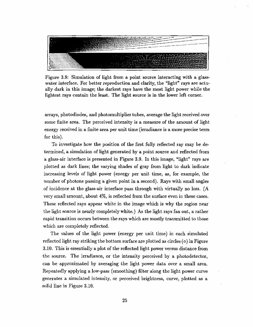
............ ~~ ....................................... .
Figure 3.9: Simulation of light from a point source interacting with a glasswater interface. For better reproduction and clarity, the "light" rays are actually dark in this image; the darkest rays have the most light power while the lightest rays contain the least. The light source is in the lower left corner.
arrays, photodiodes, and photomultiplier tubes, average the light received over
some finite area. The perceived intensity is a measure of the amount of light
energy received in a finite area per unit time (irradiance is a more precise term
for this).
To investigate how the position of the first fully reflected ray may be de
termined, a simulation of light generated by a point source and reflected from
a glass-air interface is presented in Figure 3.9. In this image, "light" rays are
plotted as dark lines; the varying shades of gray from light to dark indicate
increasing levels of light power (energy per unit time, as, for example, the
number of photons passing a given point in a second). Rays with small angles
of incidence at the glass-air interface pass through with virtually no loss. (A
very small amount, about 4%, is reflected from the surface even in these cases.
These reflected rays appear white in the image which is why the region near
the light source is nearly completely white.) As the light rays fan out, a rather
rapid transition occurs between the rays which are mostly transmitted to those
which are completely reflected.
The values of the light power (energy per unit time) in each simulated
reflected light ray striking the bottom surface are plotted as circles ( 0 ) in Figure
3.10. This is essentially a plot of the reflected light power versus distance from
the source. The irradiance, or the intensity perceived by a photodetector,
can be approximated by averaging the light power data over a small area.
Repeatedly applying a low-pass (smoothing) filter along the light power curve
generates a simulated intensity, or perceived brightness, curve, plotted as a
solid line in Figure 3.10.
25

..
250
200 Light Power
(Arbitrary 150 Units
o to 255) 100
50
100 200
Reflected light power 0
Perceived intensity -
300 . 400 5.00 600 700 DIstance from source
(Arbitrary Units, Source at 0)
800 900 1000
Figure 3.10: Locating the first fully reflected ray. The simulated light power reflected from the glass-water interface (the relative darkness of the rays striking the bottom of the image in Figure 3.9) is plotted with o's along with an approximation of the perceived brightness of the light on the outside of the wall and the point of steepest slope in the perceived brightness curve.
26

IDI --I
PC equipped wth video framegrabber digitizer, image processing software and image analysis software
, , o LED,,: ~ ~
I
... ",Uquid Surface
" . .... ~ ,":
[] \. ~u~e wall with thin, :. . , . v.tlite colting
~ LED
Figure 3.11: Schematic of the components of the film thickness system.
As can be seen in the figure, the point at which the first fully reflected ray
returns to the outer surface is marked by a very steep rise in the intensities
of the rays. If, then, the plot of light power were analyzed to determine the
point of greatest slope, the location of the first fully reflected ray could be
determined. This carries over to the plot of intensities, as weI!. The point
of greatest slope in the intensity profile is marked by a triangle (~), and it
locates the first fully reflected ray to within 4 data points or about 0.4% in
this simulation.
In addition, using this method reduces sensitivity to background light and
fouling of the test section wall while removing any direct dependence on ab
solute light intensities, thus eliminating the need for frequent calibration.
3.5 The Experimental Setup
The experimental system must perform three primary functions: the genera
tion of diffuse light rays, the capture of light reflected from the liquid surface,
and the analysis of the reflected light rays to determine the height of the liquid.
Figure 3.11 shows a schematic diagram of a possible measurement system.
Light is generated by two high-brightness light emitting diodes (LED's)
which can be easily mounted on the outside of a test section. The diffusing
lens of each LED (the rounded top) is removed down to a point very near
27

the light generating element. An opaque mask is painted onto the LED case
so that the light output is restricted to a small area directly above the light
element, preventing stray light from interfering with the measurement process.
A low-power laser may be used as the light source. Advantages include the
ability to focus the beam very tightly, better approximating a point source,
and higher brightness. It may also be possible to perform detailed analysis
on polarizing and phase shifting phenomena which could provide a significant
amount of information about the liquid surface. Care must be taken, however,
to ensure the damage threshold of the test section material is above the focused
power density of the beam. In addition, lasers containing significant energy
in the blue wavelengths may deteriorate plastics rapidly, and other materials
may be sensitive to particular common wavelengths (as Pyrex is to large power
densities in the green wavelengths). Finally, delivering the beam to the test
surface is not trivial, limiting mobility, and vibration of the test section, optics
and laser head may significantly deteriorate any accuracy gained.
A thin, light, semi-opaque coating is applied to the outer wall of the test
section. This homogenizes the light leaving the LED's and helps to distribute
light diffusely. In this particular setup, thin, frosted, plastic tape with a white
adhesive is used. Note that no air gaps can exist between the coating and the
test section wall. Even a thin air layer will cause light rays traveling at an
angle equal to or greater than the critical angle of the coating-air interface to
be reflected away from the test section, leaving very little light to enter the
test section wall at an angle such that it may arrive at the liquid-gas interface
with an angle equal to or greater than liquid-gas critical angle.
White spray paint has been used successfully for the semi-opaque coating.
The disadvantages of this are its graininess, permanence, and the difficulty
in generating an even coating. As an alternative, white spray paint has been
applied to a thin sheet of clear plastic, and this plastic sheet placed on the
test section with a thin layer of water or oil between them to act as an optical
coupling.
Since most, if not all, of the light reflected from the liquid-gas interface
will arrive at the outer wall surface at an angle greater than the critical angle
for the wall-air interface, without the coating, the light would reflect back into
the wall and thus remain trapped there. The coating then serves to couple the
28

light out of the wall and then scatter it so that an image of the reflected light
may be detected.
A video camera positioned near the test section can be used to capture
this image for further analysis. In this implementation, a small, inexpensive,
monochrome charge-coupled device (CCD) camera is mounted together with
the LED's in a single unit which can be mounted at any location on the test
section and easily moved, allowing for measurements to be taken both around
and along the test section.
The video camera output may be recorded on standard video tape, played
back, and frames selected to be measured. Whether the image analysis is
performed manually or with an automated system, it is most convenient to
use a video framegrabber peripheral to digitize the video signal and store the
image on a computer. The image can then be manipulated and enhanced by
one of the many image processing packages available.
Since using standard video recording technology can reduce image resolu
tion nearly 60% (Russ; 1994), the implemented system grabs frames directly
from the CCD camera for processing. The camera generates NTSC standard
composite video with 512 vertical lines and 486 horizontal lines, though the
limited bandwidth actually restricts the number of vertical lines to approx
imately 330 (Russ; 1994). The video framegrabber peripheral digitizes the
signal, dividing the image into picture elements, or pixels. Each pixel is as
signed a number, or numbers, specifying the brightness (if monochrome), or
color and intensity (if color), that should be displayed at that location. This
system uses a monochrome camera, so each pixel is assigned a value between
0, representing no light intensity, and 255, indicating maximum light intensity.
The image is stored in computer memory as an array of pixels, 486 elements
tall by 512 elements wide, occupying 512 x 486 = 248,832 bytes of memory.
Once stored in memory, the image can be analyzed and manipulated using
discrete mathematical operations. By applying discrete filters, the gradient
of the light intensities in the image can be generated, then the maximum
gradient located and recorded. This value must then be converted to a physical
distance, from which information about the liquid layer can be determined.
29

3.6 Image Processing Algorithm
As presented earlier, locating the first fully reflected light ray is achieved by
determining the point of greatest slope in the light intensities generated by the
reflected rays. The point of greatest slope in light intensities is found through
several image processing steps. First, the image is split into two images, one
composed of the even lines and one of the odd lines of the original image.
The brightness contrast is then enhanced and a low pass filter is applied to
the image to lessen random high frequency noise. A gradient filter is applied,
and the pixels with the largest gradient value are then selected. Finally, a
single pixel position is determined from these pixels as the point which will be
designated the point of greatest slope.
Throughout the description of the processing which follows, it will be help
ful to provide visual examples of each step. Figure 3.12 shows an actual image
of a portion of the light reflected from the surface of a moving liquid. To
demonstrate the image processing, the pixel intensity values for a single row,
row 50, have been extracted and plotted below the original image. As each
processing step is completed, a new intensity profile will be presented, clearly
showing the effect of each processing step.
3.6.1 Odd and Even Images
NTSC standard composite video is interlaced. A single standard video image is
composed of 486 horizontal lines of brightness and color which are completely
redrawn every 30th of a second. However, early television equipment was
unable to generate consecutive lines with enough precision to generate a good
image at this rate. Therefore, a standard was developed in which every other
line is drawn first, then the remaining lines filled in. Thus, during the first
60th of a second, the even lines (0, 2, ... , 486) are generated, while the odd
lines (1, 3, ... , 485) are generated in the next 60th of a second. This is what
is referred to as interlacing, or interlaced video.
When a video camera is used to capture an image of the light reflected
from the surface of a moving liquid film, essentially two images are obtained,
each a 60th of a second apart. If, for example, the film structure is moving at
0.5 mis, it will travel 8 mm from the moment the even lines are imaged till the
30

250
200
150
Pixel Value
100
50
Pixel intensity profile of row 50
Pixel Position
Figure 3.12: Processing one row of an image. The pixel intensities from row 50 of the top image have been extracted and plotted. This pixel intensity profile will be processed as an example of the processing performed to locate the position of the first fully reflected ray.
31

Figure 3.13: An interlaced image of moving liquid. This magnified view of an image of the light reflected from a moving liquid surface shows the difference in the odd and even images taken 1/60 s apart.
time the odd lines are imaged. In reality, liquid waves appear to be moving at
speeds greater than 2 or 3 m/ s. Thus, one image contains even and odd lines
representing entirely different states of the liquid. This can be clearly seen in
Figure 3.13. Fortunately, due to the way a CCD camera is implemented, all
the lines of one field, odd or even, are imaged at the same instant, rather than
over the entire 1/60 s interval.
The first step in determining the height of the liquid film, then, is to
split the captured frame of video into its even and odd fields. This is a a
straightforward operation, and provides the added benefit of giving an extra
data point for each frame-grabbing operation. Figure 3.14 shows the results
of this operation on the image in Figure 3.13.
32

Figure 3.14: Splitting an interlaced image into odd and even images. The image on the left is an interlaced image which is split into its odd (top) and even (bottom) frames on the right.
3.6.2 Brightness Contrast Enhancement
Image contrast can essentially be defined as the difference between the bright
est and darkest parts of an image. The greatest contrast a standard mono
chrome video image may have when digitized (using 8 memory bits per pixel)
is 255, which indicates that the image has at least one pixel with an intensity
of 255 (white) and at least one pixel with an intensity of 0 (black). Most im
ages have much lower contrast; perhaps maintaining a difference in intensity
between the brightest and darkest pixels of less than 100. (The contrast of the
image in Figure 3.12 of about 100 as indicated by the intensity curve plotted
below the image.)
The core of the image processing algorithm is in finding the peak gradi
ent in the light intensity. This operation is in itself relatively insensitive to
background light and should give the same maximum gradient whether the
image has low contrast or high contrast. However, with a low-contrast image,
the signal-to-noise ratio (SNR) may be very poor, making it difficult to filter
the high frequency noise from the primary intensity signal. By applying a lin
ear contrast enhancement to the image, the noise can be filtered significantly
while still maintaining a high contrast image, decreasing the susceptibility of
33
250
200
150
Pixel Value
100
50
o L-____ L-____ ~ ____ ~ ____ _L ____ _L~~~~
o 20 40 60 80 100 120 Pixel Position
Figure 3.15: Brightness profile of contrast-enhanced pixel data.
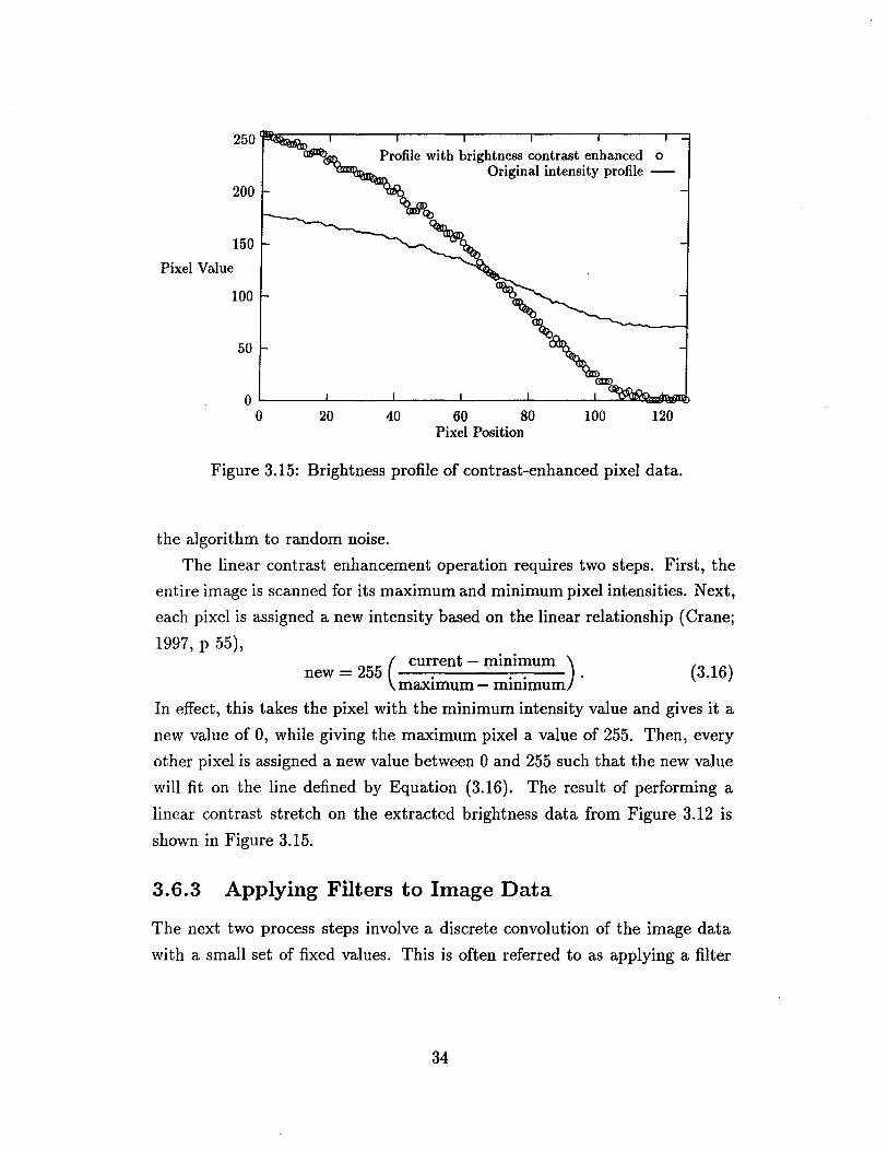
the algorithm to random noise.
The linear contrast enhancement operation requires two steps. First, the
entire image is scanned for its maximum and minimum pixel intensities. Next,
each pixel is assigned a new intensity based on the linear relationship (Crane;
1997, p 55), = 255 ( current - l;Ilinimum ) new . . . .
maXImum - mInImUm (3.16)
In effect, this takes the pixel with the minimum intensity value and gives it a
new value of 0, while giving the maximum pixel a value of 255. Then, every
other pixel is assigned a new value between 0 and 255 such that the new value
will fit on the line defined by Equation (3.16). The result of performing a
linear contrast stretch on the extracted brightness data from Figure 3.12 is
shown in Figure 3.15.
3.6.3 Applying Filters to Image Data
The next two process steps involve a discrete convolution of the image data
with a small set of fixed values. This is often referred to as applying a filter
34

to the image. Formally, the operation looks like this:
n/2 m/2
P(X, y) = ~ ~ I(i,j)F(x - i, y - j), (3.17) i=-n/2 j=-m/2
where F is a filter composed of an array of values n wide and m tall, and J is
an n x m section of the image centered at (x,y) (Gonzalez and Woods; 1992,
p 108).
To implement this, the value of the pixel at (x,y), P(x,y), is simply the
sum of the products of J(i,j) and F(i,j). Often, the final value is multiplied
by some fixed constant, or a constant is added, to give a resulting pixel value
between 0 and 255. Examples will be given in the following sections which
should help make this operation more clear.
Further simplifications and reductions in the number of computations can
be made if the filter can be written as F( i, j) = g( i)h(j). Due to the linearity of
the convolution sum, the convolution can be performed as two one dimensional
sums versus one two-dimensional sum (Gonzalez and Woods; 1992, pp 128-
130). For a 3 x 3 filter, 9 multiplications and 9 additions must be performed
for each pixel in an image. If this filter can be split into two 1 x 3 filters,
only 6 multiplications and 6 additions are required. This saves nearly 196,000
operations on a relatively small, 256 x 256 pixel image.
3.6.4 Low-Pass Filtering
Small variations in the pixel values of the image of the reflected light are not
significant to the measurement. On the contrary, these variations are magnified
many times by the gradient operation, causing difficulties in determining the
slope of the overall light intensity curve. Hence, before a gradient is performed,
a low-pass filter is applied to the image.
The filtering is achieved by an averaging operation. Each pixel is given
the value of the average of all the pixels in a neighborhood around it. A two
dimensional filter, or mask, to perform this task might be:
{
0.111 0.111 0.111 0.111 0.111 0.111
35
0.111 } 0.111 . 0.111

When this mask is convolved with the image data, a new pixel value is gener
ated equal to 1/9E(the original pixel + surrounding pixels). For example, if
the above mask is applied to the following data,
{
57 6} 6 9 3 , 374
the new pixel value for the center pixel (currently a 9) will be (0.556 + 0.778
+ 0.667 + 0.667 + 1.00 + 0.333 + 0.333 + 0.778 + 0.444) = 5.56 r~d 6.
(Pixel values must be positive integers to make sense.)
Note, however, that this same result can be achieved by using two 1 x 3
filters, one applied vertically and one applied horizontally:
{ ~1 } and {0.1l1 0.111 O.lll}. Application of the vertical filter to the
above data will give {14 23 13}. Following with the horizontal filter gives
{1.556 + 2.556 + 1.444}, or 5.56 -+ 6.
Because of the degree of smoothing required in this application, a filter of
at least 11 terms is necessary. Rather than using an 11 x 11 array, two 1 x 11
filters are used, saving 198 operations per pixel. The result of performing the
smoothing operation on the contrast-enhanced data in Figure 3.15 is shown in
Figure 3.16
For further information on how this averaging process acts as a low-pass
filter, see Appendix B.
3.6.5 The Gradient
Once the image data is smoothed, the gradient operator is applied. The con
volution method is used as it was with the low-pass filter, but with
{O 0 0 0 0 1 -1 0 0 0 0 O}
as a mask. This detects increasing light intensity from right to left in the image:
ifthe current pixel (at the -1 position in the mask) has a lower value than its left
neighbor, the sum of the two ( -1 x {current pixel} + 1 x {left neighbor}) will be
positive indicating an increase in light intensity from right to left. Decreasing
light intensity will result in a negative value and a value of zero is assigned to
36
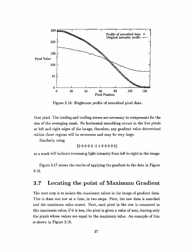
250.,.....1/JDI.Iit ___
200
150
Pixel Value
100
50
Profile of smoothed data 0 Original intensity profile -
OL---~~ __ ~ ____ ~ ____ -L ____ -L~~~=b
o 20 40 60 80 100 120 Pixel Position
Figure 3.16: Brightness profile of smoothed pixel data.
that pixel. The leading and trailing zeroes are necessary to compensate for the
size of the averaging mask. No horizontal smoothing occurs in the five pixels
at left and right edges of the image, therefore, any gradient value determined
within those regions will be erroneous and may be very large.
Similarly, using
{O 0 0 0 0 -1 1 0 0 0 0 O}
as a mask will indicate increasing light intensity from left to right in the image.
Figure 3.17 shows the results of applying the gradient to the data in Figure
3.16.
3.7 Locating the point of Maximum Gradient
The next step is to isolate the maximum values in the image of gradient data.
This is done one row at a time, in two steps. First, the row data is searched
and the maximum value stored. Next, each pixel in the row is compared to
this maximum value; if it is less, the pixel is given a value of zero, leaving only
the pixels whose values are equal to the maximum value. An example of this
is shown in Figure 3.18.
37

250
200
150
Pixel Value
100
50
Profile of the gradient of the data 0
Original intensity profile -
Pixel Position
Figure 3.17: Brightness profile of the gradient applied to the data in Figure 3.16.
250
200
150
Pixel Value
100
50
Maximum points of gradient 0
qriginal intensity profile -
(11)(II)(II)(II)(II(l1)(li)(11)
Pixel Position
Figure 3.18: Maximum values of the gradient profile in Figure 3.17.
38

250
200
150
Pixel Value
100
50
Pixel location of greatest slope 0
Original intensity profile -
o
Pixel Position
Figure 3.19: The single non-zero data point marks the pixel location of the greatest slope in the original brightness profile.
Since it is quite likely that some points of the light intensity curve are
linear, it is possible that multiple pixels will have the maximum value, as is
the case with the data in Figure 3.18. The assumption is then made that each
of these pixels belong to the same region of maximum slope. A single point
is selected by locating the edges of this region of maximum slope defined by
the first and last pixels with values equal to the maximum value and giving all
the pixels a value of zero except for the pixel at the center of the region. The
result of this selection process for the data in Figure 3.18 is shown in Figure
3.19.
This process is repeated for every row of the image, resulting in a curve
representing a section of the ring of first fully reflected light rays. Figure 3.20
shows the result of processing each row of the image that has been used as an
example in this discussion.
3.8 Defining Physical Distances
A narrow region of the reflected light image is analyzed as described above
to determine the distance between the light source and the first fully reflected
39

;' " 'oC' ' , , ~,
( ,"
<" '. , '1
) . , '" . "
.,. t
Figure 3.20: The image on the right is a result of processing each row of the image on the left as described in the text.
Figure 3.21: This image shows the processed surface reflection patterns from two light sources. The patterns represent points on the liquid surface separated by about 26 mm.
light rays. The narrow region is selected to be small enough such that curvature
effects due to the circular light ring from the source and round test section wall
distortions may be ignored. Yet the region should be large enough to average
out random noise and small, unsteady, disturbances. The analyzed image will
ideally result in a vertical line of pixels at some point in the image represent
ing the location of the reflected light rays. However, the final reflection data
may not generate a straight line due to vapor bubbles, the passage of a distur
bance wave, or poor contrast in the image. Fouling or dust may cause minor
distortions in the final image, as well. Figure 3.21 shows a typical processed
image containing the reflection patterns from two light sources. The pattern
on the left is relatively straight and its average pixel location can be used to
estimate the distance between the light source and the fully reflected light
rays. The pattern on the right, however, shows evidence of some significant
flow disturbance; perhaps a sharp wavefront or bubble.
40

It is necessary, then, to use a robust mechanism for determining the hori
zontal location of the reflected light rays. To begin with, the mean horizontal
pixel location, x, is determined for the set of pixels and the standard deviation,
u, about this mean is calculated.
Next, a deviation term is calculated for each pixel based on its location
with respect to the mean location:
IXpix - xl "'pix = 1 - 4(1 + u) . (3.18)
If "'pix < 0, it is redefined to be equal to o. This definition attempts to account
for patterned and random variations in the individual pixel locations. First,
if the pixel is far from the mean, the individual pixel should be considered
an anomaly and not heavily weighted in final calculation of the reflected light
position. The 4(1 + u) term in the denominator indicates that a pixel which
lies greater than about 4 standard deviations from the mean will be completely
ignored. Using (1 + u) instead of u prevents a singularity when the pixel lies
on the mean, and helps to prevent pixels near the mean from being eliminated
from the averaging calculation when the standard deviation is less than 1.
The horizontal location that will be defined as the point at which the first
fully reflected rays strike the outer wall, xrej, is calculated by a weighted
average of pixel locations:
(3.19)
Finally, a confidence value is assigned to the calculated location. This takes
into account the size of the standard deviation with respect to the total width
of the image to help eliminate data that is badly scattered or bi-modal.
C = L "'pix (image width - (3
)
N image width ' (3.20)
where N is the number of different pixel locations averaged together. If C < 0,
it is redefined to be equal to o. The first term is the average of the individual
pixel deviations, allowing the confidence value to account for the variation
of the individual pixels. The u3 term causes the confidence to be strongly
diminished by standard deviations greater than 1, causing scattered data to
be removed from the final reported average.
41

At this point, the distance between the source and the reflected light, x in
Equation (3.9), can be calculated from
where Xo is the location of the reflection of light from a dry wall surface, Pscale
is the pixel scale factor (mm/pixel) and Xdry is the distance between the dry
reflection point and the light source. X o, pscale, and Xdry are determined by the
calibration procedure described in Chapter 4.
After the pixel location is determined for the reflections from both light
sources, the film thickness and film slope may be calculated. Equations (3.8)
- (3.13) and (3.15) are numerically solved for the surface slope, C/>, film thick
nesses, tL, tR, and distance between reflections, Xr , using the regula falsi
method. This is an efficient step, requiring only 3 to 5 iterations. (See Scheid
(1988) for more information about the regula falsi method.)
Due to the automated nature of the measurement, several film thickness
readings may be taken quickly. The values determined for each measurement
are written to a data file along with their respective confidence values. When
the results of several measurements are averaged together, the confidence num
ber is used as a weight, so the measurements from less scattered data will have
more influence in the final result. This is calculated as
"·C·D· A
L...., , ,
verage = Ei Ci ' (3.21)
where the Ci are the confidence values corresponding to the measured data,
Di. Di may in fact be the average film thickness, tl, one of the individual film
thicknesses determined by each source, tL and tR, or the slope, c/>.
42

Chapter 4
Calibration
In theory, the optical method presented requires no calibration as it is based
entirely on the optical properties of the materials within the test section. How
ever, in practice, several details about the actual measurement apparatus need
to be known before actual distances can be calculated, and the indices of re
fraction of the wall and/or the liquid may not be known a priori. Hence, an
automated calibration procedure has also been developed to determine the
following parameters:
• Index of refraction of the test section wall material
• Index of refraction of the liquid
• Pixel scale factor (mm/pixel)
• Test section wall thickness (mm)
• Distance between each light source and its first reflected ray from a dry
surface (mm)
As a result, the only information needed prior to obtaining film thickness
data is the distance between the two light sources and one of the following:
• Index of refraction of the test section wall material
• Index of refraction of the liquid
• Test section wall thickness (mm)
43

} Figure 4.1: The top image is that of the piece of dark tape used to calibrate the pixel size of the video image. Below it is an image of the edges of the tape as determined by the image processing algorithm described previously. The tape is 12.55mm wide and the pixel scale factor is 0.0707 mm/pixel.
4.1 Obtaining the Pixel Scale Factor
Among the most critical parameters needed is the pixel scale factor which
relates a physical dimension to the pixel size. It is determined by the lens
system of the camera, the size of the CCD array and the distance between the
camera and the image. To obtain a value of the scale factor for a given set up,
an object of known width is first placed in the center of the camera's field of
view, such as the dark tape shown in Figure 4.1. Next, the image processing
algorithm described above is used to locate the edges of the tape on the screen,
as shown in the lower image of Figure 4.1. The distance between these edges
is calculated in pixels, and the pixel scale factor is calculated using the actual
physical width of the object provided by the operator. With the configuration
used to obtain the images in Figure 4.1, the distance between the edges of the
tape is 178 pixels. The tape is known to be 12.55 mm wide which gives a pixel
scale factor of 0.0707 mm/pixel.
The pixel scale factor needs only to be determined once for a given cam
era/LED set up. The factor has been found to be very consistent, even after
moving and re-mounting the camera apparatus several times.
44

4.2 Determining the Dry Wall Reference Values
From Figures 3.3 and 3.8, the distances between the light sources and the
first fully reflected rays are the primary measured values needed to calculate
the film thickness and slope. However, it is impossible to directly determine
the position of the light sources in the image frame of reference, as the light
sources are never themselves imaged. Therefore, some known reference posi
tion relative to each light source is needed. This is generated by locating the
light reflected from the dry test section wall surface. The basic algorithm for
obtaining this distance is:
• Obtain an image of the reflected light from both light sources with no
liquid on the walls
• Process the image to find the pixel locations of the reflected light images
of each source
Once these distances are known, the light sources can be located with the
knowledge of either the wall thickness and index of refraction or the distance
between the two light sources.
4.3 Determining the Unknown Properties of the Test Section and Liquid
With the dry wall reference positions known, the unknown properties of the
test section or test fluid can be determined. Beginning with the simplest case,
if either the index of refraction of the wall material, nw , or the wall thickness,
t w , is known, the other value may be calculated from
(4.1)
where Dew = sin-1(1/nw ).
If, however, both tw and nw are unknown while the index of refraction of
the liquid, nl, is known, or nl is unknown while the other two are known, some
knowledge of the light interaction with both the fluid and the wall material
must be obtained.
45

To this point, all of the liquid measurements discussed have been concerned
with the light rays completely reflected from the liquid surface. Total internal
reflection occurs at the wall-liquid interface as well. Normally, the liquid films
are thin enough that the reflected light from the wall-liquid interface is not
detected. This is due to the fact that, for films less than a transition thickness
ttl, the critical angle of the wall-liquid interface is much greater than the angle
of rays that pass through the interface and reach the liquid-vapor interface at
an angle equal to or greater than its critical angle. Therefore, the percentage
of light reflected from the wall-liquid interface is relatively small. Secondly,
the image created by these reflected rays is obscured by the brighter image
created by the rays reflecting from the surface.
The transition thickness may be derived from Figure 4.2 as follows:
X/iq = 2tw tan Oew + 2tl tan Oel
x lid = 2tw tan Oew/,
where Oewl is the critical angle for reflected light at the wall-liquid interface.
When tl = ttl, Xliq = Xlld, so, assuming a non-sloping liquid surface, setting
the above equations equal and solving for tl gives,
(4.2)
If the liquid film is thicker than ttl, the light reflected from the liquid surface
returns to the outer wall surface at a distance greater than that of the light
reflected from the wall-liquid interface, and the image of these rays reflected
from the wall-liquid interface becomes visible. This is depicted in Figure 4.2.
In operation, this places an upper bound on the thickness of liquid that can
be easily measured using the image processing algorithm described previously.
However, this phenomenon can be used to determine the remaining physical
properties of the test materials.
From Figure 4.2,
and
X lid = 2tw tan Owl.
46

:':::': ~1-r ~·r i ::":-; :";:" ::: 1-:" r ::;:"f ~T ~ ":~:~ :": ~ ':~:Tf Tf :?f 1-;- ~r~:·~·r; T :;:~'f rr ~ :~:' f Tr ~-:::1·:·1-r
'. '." FU
" :;U~' n():,'/,:, :~~~~!~,~i),n:::,', l,l,'," /
/ /
/
Figure 4.2: Light reflections when the liquid thickness is greater than ttl. The reflection of light from a dry wall has been included for reference.
Subtracting Xdry from x lid,
X lid - Xdry = 2tw tan OWl - 2tw tan Oew,
or
X lid - Xdry = 2tw (tan Owl - tan Oew). (4.3)
Now, from Snell's Law,
and
where Olw is the angle from the interface normal of the light entering the liquid
at the wall surface, and Ovw is the angle from the interface normal of the light
entering the vapor at the liquid surface.
Now, when Owl is the critical angle at the wall-liquid interface, Oew/, and
Owv is the critical angle for the wall/air interface, Oew, Olw = Ovw = 900 and
sin Olw = sin Ovw = 1. In addition, nvap = 1.000 so
and
47

Dividing the first equation by the second,
sin ()cwl nl = . () .
SIn cw (4.4)
Equations (4.1), (4.3) and (4.4) are completely defined if the distances Xdry
and x lid are determined by measurement and one of the indices of refraction,
nl or n w , or the wall thickness, t w , is known. Hence, this part of the calibration
procedure requires the following basic steps:
• Obtain an image of the reflected light with a liquid layer greater than the
wall thickness (greater than ttl) in the test section (assuming the steps
above for the dry wall have been completed).
• Process this image to determine x lid, the distance between the reflected
rays and the light source.
• Request input from the experimenter. At least one of the following must
be given:
- Index of refraction of the wall material
- Index of refraction of the liquid
- Thickness of the wall
• Solve the appropriate set of equations to determine the missing data,
if any. (The experimenter may choose to enter all of the material and
liquid properties.)
Solving for tw or nw from Equation (4.1) is quite simple. If Equations (4.1),
(4.3) and (4.4) need to be solved simultaneously for two unknowns, however,
the regula falsi method is used to numerically solve the equations. The regula
falsi method is described by Scheid (1988).
4.4 Implementation of the Calibration Procedure
The calibration procedure is implemented in a manner designed to be con
venient for the experimenter and to lessen the chance of uncertainty in the
48

measurements. First, the pixel scale factor must be determined. Once deter
mined for a given set-up, it is generally unnecessary to repeat this operation.
Next, the experimenter is presented with three options:
1. Perform the dry wall calibration
2. Perform the flooded wall calibration
3. Determine tw , nl and nw
If a completely new test section and new liquid are to be measured, each
step must be performed. However, the flooded wall calibration is required only
when two of the properties are unknown and need to be determined, and step
3 is only required when a new test section or liquid is used. If the properties of
the new test section and fluid are known a priori, those values may be entered
directly without performing the flooded wall calibration.
Experience has shown that the dry wall calibration should be performed
with each new camera placement. Essentially, this serves to "zero" the mea
surement by defining the dry wall reflection positions. This compensates for
any movement of the camera relative to the LED's that might have occurred in
re-mounting the apparatus. If the wall is not of uniform thickness throughout
the test section, steps 1 and 3 need to be performed at each new measurement
location to adjust the value of the wall thickness, two
Finally, this calibration procedure can be used to determine the index of
refraction of any liquid that does not significantly reflect or absorb the light
generated by the LED's. A test apparatus for this purpose can be constructed
of a material with known wall thickness and index of refraction, and steps 2
and 3 performed to determine the test liquid's index of refraction.
49

Chapter 5
Experimental Validation and Analysis
5.1 The Experimental System
The components necessary for implementing this film thickness measurement
system have been introduced in Section 3.5. This section details the construc
tion of the experimental measurement system.
High brightness LED's from Radio Shack (part number 276-087) with a
typical wavelength of 660 nm are used for the two light sources. These are
powered from the same 12 volt power supply used by the camera. Two 150
ohm resistors in series with the LED's limit the current, though not below
the suggested maximum operating current level. This was done to obtain high
intensities while knowingly shortening the life of the LED's. During the course
of the initial experimental work, the LED's appeared to have a limit of about
50 to 100 working hours before their intensities fell below the required level.
Other LED sources may provide greater intensities at lower currents, thus
enhancing component lifetimes.
The LED casings must be modified so that a point source of light may be
placed at the test section wall. First, the rounded top of the LED is removed to
just above the light emitting element. Then, the case is painted black except
for the area immediately above the emitting element. The LED's are then
mounted approximately 3 cm above the camera lens using a short piece of 1
inch schedule 40 PVC pipe.
The video camera is an inexpensive, monochrome CCD camera in 1/3
50

Mounting Plate
o o
o o
Figure 5.1: Important features of the camera assembly. Side view on the left, top view on the right.
inch format with an adjustable micro-lens. The CCD array is made up of
420 horizontal rows by 360 vertical columns of sensors. The output of this
array is converted to 512 horizontal lines by 486 vertical lines by the camera
electronics to generate NTSC standard interlaced output. These cameras are
typically sold for surveillance or hobby applications and can be purchased quite
reasonably from surplus supply companies. The camera is supplied with 12
VDC with a 600 mA wall transformer. A small plastic box with a hole in the
lid just large enough for the camera and ventilation holes in its sides and back
is used as a housing, with the LED holder fastened to the lid. The important
features of the camera assembly are shown in Figure 5.l. . The camera box is then secured to a mounting plate with 4 holes drilled
in it to allow the camera assembly to be mounted to the side of a test section.
Figure 5.2 shows the camera assembly mounted to a cylindrical test section.
The backside mounting support is fabricated from a 4 inch PVC coupling, cut
in half, with 4 holes drilled to mate with the holes in the camera mounting
base. Four bolts through these holes secure the camera to the test section.
Two lengths of 1/4 inch PVC have been glued to the top center of the back
support to ensure that the assembly is centered and aligned with the axis of
the test section.
Video data from the camera is acquh:~d and digitized by a Truevision
Targa+ image capture card (often called a framegrab ber ). When processing
monochrome data, the Targa+ uses 8 bits to encode the gray level informa-
51

Figure 5.2: Mounting the camera assembly to a cylindrical test section.
tion in the image. Thus, each image pixel is assigned a value between 0 (no
light) and 255 (maximum light intensity). An IBM-compatible computer with
a 486sx microprocessor, 8 Mb of RAM and 100 Mb of hard disk storage is used
to control the framegrabber and process the images.
Custom software has been written to access the framegrabber and im
plement the image processing algorithm described in Section 3.6. Including
debug code and documenting comments, the film thickness measurement soft
ware contains over 3000 lines of C++ code. This may be compiled using the
reasonably standard and freely available Gnu C++ compiler from the Free
Software Foundation 1. This software implements about 20 different image
manipulation functions. The user may then create a custom image process
ing system for each measurement application by combining these functions.
Commands may be issued via a standard input file or interactively from the
keyboard.
As implemented, each image is processed in approximately 9 seconds, but
1 As it is impractical and fairly useless to include so much code in this document, the software will be made available via the Internet. The author or advising professor may be contacted through the Mechanical and Industrial Engineering department for more information.
52

Measured Measured Software Software Difference Width Scale Width Scale in Scale (pixels) Factor (pixels) Factor Factor
166 0.0757 164 0.0766 1.2% 173 0.0726 176 0.07136 -1.7% 173 0.0726 178 0.0706 -2.8% 179 0.0702 177 0.0708 0.9%
Table 5.1: Verification of the pixel scale factor calibration procedure
this may be shortened to about 4 seconds if intermediate images do not need
to be saved or viewed. Each image will contain an even and odd field, with
each field displaying light reflected from each of the two LED's, so four mea
surements are actually made with each image acquisition. Data from many
images may be stored and averaged together as discussed in Section 3.8.
5.2 Experimental Validation
Both the experimental system and the proposed film thickness measurement
method must be validated. This is achieved by attempting to confirm the
functionality of each system component, as well as confirming that the method
generates results consistent with known data.
5.2.1 Calibration Parameters
The Pixel Scale Factor
The pixel scale factor is determined as described in Section 4.1. Verification of
this measurement and calculation is performed by acquiring an image of the
reference object and displaying it on a monitor. The image on the monitor is
manually measured using calipers and then converted to an equivalent width
in pixels. For the monitor used, 1 cm = 16 pixels. The known width of the
reference object (12.56 mm) is then divided by the pixel width of the object
which results in the pixel scale factor. This is then compared with the result
generated by the image processing software. The results are presented in Table
5.1.
The agreement between the software and manual measurements is quite
53

good, especially since the caliper readings have an uncertainty of about 3% in
this range. This indicates that the image processing algorithm is accurately
locating the sharp change in contrast and is able to accurately and consistently
determine pixel locations for the object edges.
Some variation is noted in the pixel scale factors listed in the table. The
largest variations were the result of finding the pixel scale with the reference
object placed lightly on top of the camera assembly, versus securing the ref
erence object with bolts. The compression of the tape, camera box lid, and
other structures brings the reference object a little closer to the camera, thus
decreasing the pixel scale factor. In actual use, the camera is secured in nearly
the same fashion each time it is re-mounted, so pixel scale variations are very
small.
Determination of Unknown Material Properties
The calibration procedure described in Section 4.3 will determine two of three
important material parameters using measured reflections from both a dry
wall and a wall with a thick layer of fluid on it.
In each of the following cases, the wall material is acrylic (methyl methacry
late) and the liquid is water. Acrylic has a refractive index of nw = 1.489 in
the red wavelength (ASM International Handbook Committee; 1988, p.596),
while water has a refractive index of nl = 1.330 (Weast; 1983, p.E-362).
In general, the data of Table 5.2 indicates that the calibration procedure
works quite well. In gathering the data, it has been found that much of the
error and inconsistency in the calibration results comes from the measurement
of the distance between the two sources. One issue is the determination of ex
actly which two points should be used as the reference points on the sources.
For example, an argument could be made from the paths of the light rays
that the correct distance is the distance between the outside edges of the light
emitting elements. However, this is difficult to verify, and did not always give
consistent results. Another issue is the difficulty of physically measuring this
distance, whether by using calipers to measure points on the sources or calcu
lating the source positions by measuring distances between the reflected light
rings. Finally, it seems to be fairly certain that the sources in the experimental
apparatus used are not securely mounted enough to prevent slight movement
54

Given Found Error
nl = 1.33 nw = 1.50 0.7%
tw = 3.2 mm nl = 1.33
nw = 1.489 0.0% tw = 6.05 mm
nl = 1.33 nw = 1.51 1.4%
tw = 3.235 mm 1.1%
tw = 2.94 mm nl =.1.297 -2.4% nw = 1.460 -2.0%
tw = 2.94 mm nl = 1.306 -1.8% nw = 1.469 -1.3%
nl = 1.33 nw = 1.52 2.1%
tw = 3.17 mm 7.8%
tw = 2.95 mm nl = 1.337 0.5% nw = 1.503 1.0%
tw = 2.95 mm nl = 1.331 0.1% nw = 1.499 0.7%
Table 5.2: Using the calibration procedure to determine unknown material properties.
when the camera assembly is firmly mounted to a test section. Movements
of a few tenths of a millimeter can mean significant errors in the calibration
results.
To verify the use of this system with a material other than acrylic, the index
of refraction of a piece of clear PVC has been calculated. The thickness of the
PVC is determined to be 5.94 mm. Two separate calibration measurements
generated nw = 1.575 and nw = 1.552. The refractive index of blue tinted
clear PVC is about 1.53 (Nass; 1977, p.723), though the exact composition of
the PVC is not known.
5.3 Film Thickness Measurements
5.3.1 Static Liquid Measurements
Measurement Procedure
Figure 5.3 shows the apparatus used to compare the measurements made us
ing the automated optical system with those made using the needle-contact
55

Conductivity Sensing ~~~"., Orcuit
SUpport stand
Test
=::J~~~~~~Contalner
Figure 5.3: Setup for static liquid film measurements.
method. The camera assembly rests on the base of a stand and an open, shal
low container is placed on the LED holder. A metric dial caliper with a needle
attached is mounted from the stand above the liquid container. The needle
is connected to one terminal of a conductivity sensing circuit, while the other
terminal of the circuit is in contact with the water. When the needle first
touches the water surface, an indicator will light. The caliper assembly can
be moved to measure the film thickness at either the left or right light source
positions.
After calibrating the optical system to the container wall, the measure
ments proceed as follows:
• Locate the left surface reflection point (about half the distance between
the source and the reflected light ring).
• Lower the needle until it first comes in contact with the water. Note dial
reading.
• Lower the needle until it first touches the wall. Note the reading.
• Repeat these steps 5 to 10 times.
56
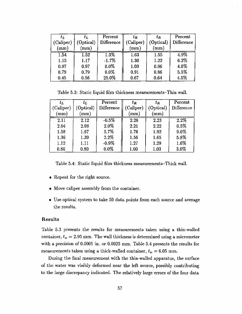
tL tL Percent tR tR Percent (Caliper) (Optical) Difference (Caliper) (Optical) Difference
(mm) (mm) (mm) (mm)
1.54 1.52 1.3% 1.63 1.55 4.9% 1.15 1.17 -1.7% 1.30 1.22 6.2% 0.97 0.97 0.0% 1.00 0.96 4.0% 0.79 0.79 0.0% 0.91 0.86 5.5% 0.45 0.56 25.0% 0.67 0.64 4.5%
Table 5.3: Static liquid film thickness measurements-Thin wall.
tL tL Percent tR tR Percent (Caliper) (Optical) Difference (Caliper) (Optical) Difference
(mm) (mm) (mm) (mm) 2.11 2.12 -0.5% 2.28 2.23 2.2% 2.04 2.08 2.0% 2.21 2.22 0.5% 1.58 1.67 5.7% 1.76 1.92 9.0% 1.36 1.39 2.2% 1.56 1.65 5.8% 1.12 1.11 -0.9% 1.27 1.29 1.6% 0.80 0.80 0.0% 1.00 1.03 3.0%
Table 5.4: Static liquid film thickness measurements-Thick wall.
• Repeat for the right source.
• Move caliper assembly from the container.
• Use optical system to take 50 data points from each source and average
the results.
Results
Table 5.3 presents the results for measurements taken using a thin-walled
container, tw = 2.95 mm. The wall thickness is determined using a micrometer
with a precision of 0.0001 in. or 0.0025 mm. Table 5.4 presents the results for
measurements taken using a thick-walled container, tw = 6.05 mm.
During the final measurement with the thin-walled apparatus, the surface
of the water was visibly deformed near the left source, possibly contributing
to the large discrepancy indicated. The relatively large errors of the four data
57

2m
\ Camera Wet Assembly Vacuum
4m
Figure 5.4: Schematic of Horizontal air-water flow loop.
points in the center of the the thick-walled data set may be attributable to
the uncertainty in the caliper measurements. The caliper appears to have
an uncertainty of about 0.05 mm. For the two sets of data with differences
consistently greater than 2.0%, only 5 data points were taken with the caliper.
At least 7 data points were taken for the remaining data in both tables.
Overall, the optically measured data agree with the contact data to within
3.9%. If the five data points that have been questioned due to possible experi
mental error are excluded, agreement is within 2.3%. This is within the range
of the apparent uncertainty of the caliper used, and is better than much that
is reported in the literature for various film measurement techniques (gener
ally 5% to 10%). See, for example, Coney et al. (1989); Paras and Karabelas
(1991); Himmelsbach et al. (1994); and Evers and Jackson (1995).
5.3.2 Flowing Film Measurements
Measurement Procedure
A horizontal air-water flow loop, depicted in Figure 5.4, has been constructed
to study the liquid film distribution in horizontal, annular, two-phase flow in
passages of varying sizes and geometries. The loop consists of about 7.5 m
of 38.1 mm J.D. PVC pipe on the air inlet side. Pressure taps 2 m apart are
connected to an inclined, water-filled manometer to give the pressure drop
through this section. Water is injected circumferentially into the test section
from a raised reservoir. The test section consists of about 4.9 m of 25.3 mm
J.D. acrylic tubing. Pressure taps 1 m apart are connected to a vertical water-
58

filled manometer. The vapor flow is driven by a 6.0 HP Craftsman Wet-Vac.
A sump pump in the wet-vacuum tank is actuated by a float switch to refill
the reservoir.
Air flow characteristics are obtained using the pressure information from
the inlet section. The pressure drop, air density and temperature can be used
with relations for the Fanning friction factor, mass flow rate and Reynold's
number to solve for the mass flow rate of air through the system. Liquid mass
flow rates are determined by timing the fall of the liquid level in the reservoir.
The measurements of mass flow rates are believed to be accurate to better
than 5%.
Results
Liquid film thickness data is measured 4 m from the beginning of the test
section, about 160 LID's. The camera assembly is mounted on the tube as
shown in Figure 5.2, and 25 images are analyzed at 8 radial locations, each
separated by 45°. Thus, the average of 100 measurements is used at each
location to calculate the average film thickness, h. The measurement results
are given in Figure 5.5.
Aside from the shift in the peak film thickness, the measured data fol
lows the trends of the other researchers well. The measured flow distribution
appears to be rotated about 45° from what .would be expected, and no clear
explanation can be given. However, it should be noted that the data presented
by Fukano and Ousaka, as well as Hurlburt and Newell, only include half the
cylinder and are assumed to be symmetric. Data presented by Dallman (1978)
indicate some asymmetry, though he only provides one additional radial point
to compare with.
Fukano and Ousaka measure significantly thinner films on the top of their
test section. This is possibly explained by the fact that their test section had
an inner diameter of 26 mm, versus the 25.3 mm used in this experiment, as
well as by the higher air flow used in their work. In addition, Fukano and
Ousaka used conductance probes to obtain their data and this measurement
method may be prone to under-predicting the film thickness in thin liquid
films due to the wavy surface and entrained air bubbles.
Hurlburt and Newell obtained their data using the optical technique on
59

0.3
0.28
0.26
0.24
0.22 h 0.2 (mm)
0.18
0.16
0.14
0.12
0.1 0 50 100 150
x Measured -e-Fukano and Ousaka; 1989 -A
Hurlburt and Newell; 1996 X X
200 250 300 350
Radial Location (Degrees, Top of tube at 0)
Figure 5.5: The film thicknesses measured around the test section are plotted together with representative data from the literature. The measured flow conditions are rna = 0.021 Kg/s, rnl = 0.019 Kg/s. The Fukano and Ousaka data is taken from a flow with rna = 0.025 Kg/s, rnl = 0.019 Kg/s. Hurlburt and Newell measured a flow with rna = 0.020 Kg/s, ml = 0.013 Kg/s.
60

which the current measurements are based and found thicker films in general.
However, it is possible that the thicker film measurements they report can
be attributed to overestimating the size of the reflected light ring, since the
measurement of the ring was performed manually. Further, their data was
obtained using fewer samples of the optical signal and at a location on the
test section with much shorter development length. Finally, it is possible
that, because of the algorithm described in Section 3.8 used to eliminate noisy
optical signals, the automated system may tend to filter out thicker waves on
the liquid surface, thus giving a thinner average film thickness.
5.4 Sensitivity Analysis
As is apparent from the discussion of the image processing algorithm in Sec
tion 3.6 and the calibration procedure in Chapter 4, the calculation of accurate
film thicknesses is dependent upon many parameters. In an effort to under
stand how the film thickness calculation is affected by the different measured
quantities, a single test case has been analyzed by varying input quantities
over a known range. Similarly, the sensitivity of the calibration procedure to
variations in input values has been performed. The results of these analyses
are given in Appendix C.
In summary, changes of ± 5% in nl or nw will cause changes of about 10%
in the film thicknesses calculated. From the calibration analysis, errors of 5%
in the determination of nl or nw are possible if the measurement of darc or
pacale is in error by 5% and neither nl or nw are known beforehand.
A 5% error in the knowledge of either tw or Pacale will be reflected as about
a 5% deviation in the calculated film thicknesses. Determining an unknown
tw using the calibration procedure is very sensitive to almost all parameters.
A 5% difference in nl, n w , darc or pscale will generate errors of 10% to 20% in
the value of tw thus determined.
If, for some reason, the image processing algorithm for determining the
position of the first fully reflected ray is off by 5 pixels, the film thicknesses
calculated will be in error by about 7%. Finally, the film thickness calculations
are most sensitive to changes in darc. A 5% variation in darc will generate about
a 15% difference in the film thickness values.
61

Chapter 6
Conclusions
6.1 Summary
An automated optical liquid film thickness measurement system has been pre
sented both in theory and application. Compared with other techniques cur
rently available for measuring thin liquid films, this optical system shows ad
vantages in flexibility and precision. The method is not limited to a particular
fluid or flow configuration, as long as a test section with transparent walls
is available and the fluid does not heavily absorb or scatter the light at the
wavelengths used. With a precision of about 30 microns, very thin films may
be measured. In addition, using large numbers of averaged data points, films
on the order of 30 microns or less may be- measured with statistical confi
dence. This precision limit is determined primarily by the camera lens and
CCD array. Greater precision may be obtained with a larger array or a lens
system with greater magnification. As implemented, liquid films have been
measured which agree with needle-contact measurements to within about 3%.
In addition, good agreement with published data is shown for measurements
of flowing films.
The implementation described uses two separate light sources. From the
data collected and the sensitivity analysis that has been performed, it is rec
ommended that future systems use a single LED, if possible, due to the errors
that can be associated with uncertainties in the knowledge of the distance be
tween the two sources. This, however, will limit the application of the method
to films less than about 2 mm and test section wall thicknesses of about 4 mm
or less. The dual light source system maybe used with thicker walls and films,
62

but care must be taken in determining the source separation.
6.2 Other Applications
This work has led to the development of other potential applications of the
theory used for the film thickness measurement. As shown in Figure 6.1, it
seems possible to derive a profile of the flowing liquid surface using the image
processing techniques that have been developed. Several issues need to be
resolved yet before the images can be directly correlated to the fluid surface,
but it is apparent that fine structure and much qualitative information can be
ascertained quite simply.
Other possible applications include the determination of liquid properties
through the use of surface profiling, concentration measurement by detecting
changes in index of refraction, and manufacturing process monitoring.
63

UquldRow ,
TOP
:. :~
.~.,
Transparent - ~indricaJ _
Test Section
liquid Flow , Liquid Film
/ ' .... LED ...... ....
SIDE
Camera
Figure 6.1: These images are the result of processing video data taken in the axial direction. The test section wall is on the left side of each image and the flow direction is from top to bottom.
64

Appendix A
The Angle at the Wall-Liquid Interface
Earlier it was emphasized that the angle with which the light ray that reflects
from the liquid surface at the liquid-air critical angle approaches the wall
liquid interface is the critical angle corresponding to a wall-air interface. This
can be shown with reference to Figure A.I. First, from Snell's Law,
nl sin Olw = nw sin Owl'
If the liquid surface is parallel to the wall surface,
because they are opposite interior angles of two parallel lines. Substituting,
But, Oel is the critical angle for the liquid air interface, so
O . -1 ( 1 ) el = SIn -. nl
This, then, gives . ( • -1 ( 1 )) . 0 nlsm sm - = nwsm wi
nl
1 . 0 nl . - = nw SIn w nl
sinOwI=(~)' nw
65

Figure A.I: Angles of the light ray that will reflect from the liquid surface at the critical angle
Since nair = 1, this can be written
. 0 nair SIn wi = --.
nw
Now, by comparison with the equation defining the critical angle, (3.2),
. 0 n2 SIn e = -,
nl
it is evident that Owl must be equal to the critical angle at the wall-air interface,
Oew.
Note that this is true only for the first fully reflected light ray, which is the
only light ray to reflect from the liquid-air interface at the critical angle Oel.
66

Appendix B
Low Pass Filter Behavior of the Averaging Filter
The averaging operation has been described as acting as a low . pass filter.
This can be shown as follows. In one dimension, using the definition of the
convolution sum, Equation (3.17), the averaging operation can be written as
N
P(x) = E I(i)F(x - i) = 1* F. i=-N
F( x), the averaging filter, can be described formally as
F() {I if - N < x < N x = 0 otherwi~e .
(B.l)
The image data, I(x), contains W pixels, and the * indicates convolution.
Taking the Fourier transform of (B.l), p(n) = 1(n)F(n), since the convolu
tion in the spatial domain becomes multiplication in the frequency domain.
1(0,) is the power spectrum of the frequencies contained in the image data,
while the transform of the averaging filter is given by
F(n) = sin[n(N + !)] . sin(n/2)
(B.2)
(See, for example, Oppenheim, Willsky and Young; 1983, p 339.) The spatial
frequency, 0" is given by 0, = 27rk
W' where W is the total number of pixels in the row or column being analyzed
and k is the index of the discrete frequency points along the transformed data.
67

F(f2)
12
10
8
6
4
2
0
-2
-4
-6 0 2'71"
"3
sin[n(N + k )] sin(n/2)
Figure B.1: The Fourier transform of the averaging filter
For instance, if W = 500 and k = 20, the corresponding frequency would be
f2 = 0.087r radians, or 0.04 cycles/pixel. Equation (B.2) is plotted in Figure
B.1. After multiplying F and I, then, the lower frequency components of the
image data will dominate and the averaging filter does indeed act as a low-pass
filter.
68

Appendix C
Sensitivity Analysis Data
nl 1.330 nw 1.490 tw 2.95 mm
Pscale 0.075 mm/pixel dsrc 32.5 mm
¢> 0.432° tL 2.269 mm tR 2.433 mm Xr 21.793 mm
Table C.1: Base data set for measurement sensitivity analysis.
Base -5% % chg -1% % chg 1% % chg 5% % chg nl 1.330 1.264 -5.000 1.317 -1.000 1.343 1.000 1.397 5.000
</J 0.432 0.381 -11.806 0.422 -2.315 0.442 2.315 0.480 11.111 tL 2.269 1.998 -11.944 2.216 -2.336 2.320 2.248 2.522 11.150 tR 2.433 2.143 -11.919 2.377 -2.302 2.488 2.261 2.700 10.991 Xr 21.793 21.794 0.005 21.793 0.000 21.793 0.000 21.793 0.000
Table C.2: The effect of varying nl on liquid film measurements.
69

Base -5% %chg -1% % chg 1% % chg 5% % chg nw 1.490 1.416 -5.000 1.475 -1.000 1.505 1.000 1.565 5.000
<P 0.432 0.433 0.231 0.433 0.231 0.433 0.231 0.432 0.000 tL 2.269 2.038 -10.181 2.236 -1.454 2.320 2.248 2.466 8.682 tR 2.433 2.203 -9.453 2.400 -1.356 2.485 2.137 2.630 8.097 Xr 21.793 21.770 -0.106 21.769 -0.110 21.770 -0.106 21.781 -0.055
Table C.3: The effect of varying nw on liquid film measurements.
Base -5% % chg -1% % chg 1% %chg 5% % chg
tw 2.950 2.803 -5.000 2.921 -1.000 2.980 1.000 3.098 5.000
<P 0.432 0.433 0.231 0.433 0.231 0.433 0.231 0.433 0.231 tL 2.269 2.400 5.773 2.301 1.410 2.269 0.000 2.170 -4.363 tR 2.433 2.564 5.384 2.466 1.356 2.433 0.000 2.334 -4.069 Xr 21.793 21.760 -0.151 21.772 -0.096 21.740 -0.243 21.751 -0.193
Table C.4: The effect of varying tw on liquid film measurements.
Base -5% % chg -1% % chg 1% % chg 5% % chg d. rc 32.500 30.875 -5.000 32.175 -1.000 32.825 1.000 34.125 5.000
<P 0.432 0.450 4.167 0.435 0.694 0.430 -0.463 0.417 -3.472 tL 2.269 1.940 -14.500 2.203 -2.909 2.367 4.319 2.630 15.910 tR 2.433 2.104 -13.522 2.367 -2.713 2.532 4.069 2.795 14.879 Xr 21.793 20.918 -4.015 21.618 -0.803 21.893 0.459 22.593 3.671
Table C.5: The effect of varying dare on liquid film measurements.
Base -5% % chg -1% % chg 1% % chg 5% % chg
P.cale 0.075 0.071 -5.000 0.074 -1.000 0.076 1.000 0.079 5.000
<P 0.432 0.416 -3.704 0.430 -0.463 0.436 0.926 0.450 4.167 tL 2.269 2.405 5.994 2.311 1.851 2.258 -0.485 2.175 -4.143 tR 2.433 2.561 5.261 2.474 1.685 2.424 -0.370 2.347 -3.535 Xr 21.793 21.492 -1.381 21.698 -0.436 21.815 0.101 21.997 0.936
Table C.6: The effect of varying Paeale on liquid film measurements.
Base -5 pix. % chg -1 pix. % chg 1 pix. % chg 5 pix. % chg
PL 89 84 -5 pix 88 -1 pix 90 1 pix 94 5 pix PR 236 241 -5 pix 237 -1 pix 235 1 pix 231 5 pix
<P 0.432 0.425 -1.620 0.431 -0.231 0.434 0.463 0.440 1.852 tL 2.269 2.104 -7.272 2.236 -1.454 2.301 1.410 2.433 7.228 tR 2.433 2.269 -6.741 2.400 -1.356 2.466 1.356 2.597 6.741 Xr 21.793 22.168 1.721 21.868 0.344 21.718 -0.344 21.418 -1.721
Table C.7: The effect of varying the reflection pixel locations on liquid film measurements.
70
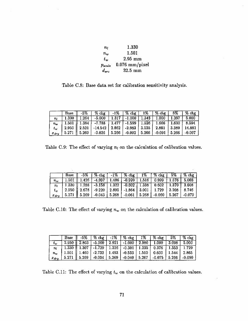
nz 1.330 nw 1.501 tw 2.95 mm
PscaZe 0.076 mm/pixel darc 32.5 mm
Table C.8: Base data set for calibration sensitivity analysis.
Base -5% %chg -1% % chg 1% % chg 5% % chg nl 1.330 1.264 -5.000 1.317 -1.000 1.343 1.000 1.397 5.000 nw 1.501 1.384 -7.788 1.477 -1.599 1.526 1.666 1.630 8.594 tw 2.950 2.521 -14.542 2.862 -2.983 3.035 2.881 3.389 14.881
Xdry 5.271 5.269 -0.036 5.266 -0.092 5.266 -0.091 5.266 -0.097
Table C.9: The effect of varying nz on the calculation of calibration values.
Base -5% % chg -1% % chg 1% % chg 5% % chg nw 1.501 1.426 -4.997 1.486 -0.999 1.516 0.999 1.576 5.003 nl 1.330 1.288 -3.158 1.322 -0.602. 1.338 0.602 1.370 3.008 tw 2.950 2.678 -9.220 2.895 -1.864 3.001 1.729 3.208 8.746
Xdry 5.271 5.269 -0.043 5.268 -0.061 5.268 -0.060 5.267 -0.079
Table C.lO: The effect of varying nw on the calculation of calibration values.
Base -5% % chg -1% % chg 1% % chg 5% % chg tw 2.950 2.803 -5.000 2.921 -1.000 2.980 1.000 3.098 5.000 nl 1.330 1.307 -1.729 1.326 -0.301 1.335 0.376 1.353 1.729 nw 1.501 1.460 -2.732 1.493 -0.533 1.510 0.600 1.544 2.865
Xdry 5.271 5.269 -0.034 5.269 -0.040 5.267 -0.075 5.266 -0.090
Table C.ll: The effect of varying tw on the calculation of calibration values.
71

Base -5% % chg. -1% % chg. 1% % chg. 5% % chg.
P.cale 0.076 0.072 -5.000 0.075 -1.000 0.077 1.000 0.080 5.000 nl 1.330 1.330 0.000 1.330 0.000 1.330 0.000 1.330 0.000 nw 1.501 1.549 3.198 1.510 0.600 1.493 -0.533 1.462 -2.598 tw 2.950 3.442 16.678 3.042 3.119 2.858 -3.119 2.517 -14.678
Xdry 5.271 5.819 10.406 5.377 2.021 5.156 -2.179 4.720 -10.449 nl 1.330 1.307 -1.729 1.325 -0.376 1.335 0.376 1.354 1.805 nw 1.501 1.501 0.000 1.501 0.000 1.501 0.000 1.501 0.000 tw 2.950 3.256 10.373 3.010 2.034 2.887 -2.136 2.641 -10.475
Xdry 5.271 5.818 10.373 5.378 2.034 5.158 -2.136 4.719 -10.475 nl 1.330 1.268 -4.662 1.316 -1.053 1.345 1.128 1.412 6.165 nw 1.501 1.424 -5.130 1.484 -1.133 1.519 1.199 1.601 6.662 tw 2.950 2.950 0.000 2.950 0.000 2.950 0.000 2.950 0.000
Xdry 5.271 5.820 10.415 5.381 2.089 5.160 -2.101 4.719 -10.470
Table C.12: The effect of varying Pacale on the calculation of calibration values first assuming a known nl, next a known nw , and finally, a known two
Base -5% % chg. -1% % chg. 1% %chg. 5% % chg. d. rc 32.500 30.875 -5.000 32.175 -1.000 32.825 1.000 34.125 5.000 nl 1.330 1.330 0.000 1.330 0.000 1.330 0.000 1.330 0.000 nw 1.501 1.460 -2.732 1.492 -0.600 1.510 0.600 1.547 3.065 tw 2.950 2.370 -19.661 2.828 -4.136 3.071 4.102 3.588 21.627
Xdry 5.271 4.456 -15.461 5.108 -3.088 5.429 2.994 6.080 15.345 nl 1.330 1.355 1.880 1.335 0.376 1.325 -0.376 1.308 -1.654 nw 1.501 1.501 0.000 1.501 0.000 1.501 0.000 1.501 0.000 tw 2.950 2.494 -15.458 2.857 -3.153 3.053 3.492 3.403 15.356
Xdr!! 5.271 4.456 -15.458 5.105 -3.153 5.455 3.492 6.080 15.356 nl 1.330 1.445 8.647 1.350 1.504 1.312 -1.353 1.252 -5.865 nw 1.501 1.659 10.526 1.528 1.799 1.477 -1.599 1.393 -7.195 tw 2.950 2.950 0.000 2.950 0.000 2.950 0.000 2.950 0.000
Xdry 5.271 4.457 -15.438 5.107 -3.112 5.428 2.980 6.084 15.427
Table C.13: The effect of varying darc on the calculation of calibration values first assuming a known nl, next a known n w , and finally, a known two
72

Bibliography
Andritsos, N. (1985). Effect of Pipe Diameter and Liquid Viscosity on Horizon
tal Stratified Flow, PhD thesis, University of Illinois at Urbana-Champaign,
Urbana,IL.
ASM International Handbook Committee (1988). Engineering Plastics, Vol. 2
of Engineering Materials Handbook, ASM International, Metals Park, OH.
Azzopardi, B. J. (1986). Disturbance wave frequencies, velocities and spac
ing in vertical annular two-phase flow, Nuclear Engineering and Design
92(2): 121-133.
Barter, J. D. and Lee, P. H. Y. (1994). Real-time wave-amplitude spectrum
analyzer for air-liquid interfaces, Applied Physics Letters 64(15): 1896-1898.
Bousman, W. S., McQuillen, J. B. and Witte, L. C. (1996). Gas-liquid flow
patterns in microgravity: Effects of tube diameter, liquid viscosity and sur
face tension, International Journal of Multiphase Flow 22(6): 1035-1053.
Brown, R. C., Andruessi, P. and Zanelli, S. (1978). The use of wire probes
for the measurement of liquid film thickness in annular gas-liquid flows, The
Canadian Journal of Chemical Engineering 56: 754 - 757.
Chen, X., Butler, T. and Brill, J. P. (1996). Capacitance probes for measure
ment of liquid film thickness, HTD- Vol 334, Proceedings of the ASME Heat
Transfer Division at the International Mechanical Engineering Congress and
Exposition, Vol. 3, ASME, Atlanta, GA, pp. 201-208.
Chun, M.-H. and Sung, C.-K. (1986). Parametric effects on the void fraction
measurement by capacitance transducers, International Journal of Multi
phase Flow 12(4): 627-640.
73

Coney, J. E. R., EI-Shafei, E. A. M. and Sheppard, C. G. W. (1989). A dual
laser beam method for wavy film thickness measurement, Optics and Lasers
in Engineering 11: 1-14.
Coney, M. W. E. (1973). The theory and application of conductance probes
for the measurement of liquid film thickness in two phase flow, Journal of
Physics E: Scientific Instruments 6: 903 - 910.
Crane, R. (1997). A simplified approach to image processing, first edn, Prentice
Hall PTR, Upper Saddle River, N J.
Dallman, J. C. (1978). Investigation of Separated Flow Model in Annular
Gas-Liquid Two-Phase Flows, PhD thesis, University of Illinois at Urbana
Champaign, Urbana, IL.
Driscoll, D. I., Schmitt, R. L. and Stevenson, W. H. (1992). Thin flowing liquid
film thickness measurement by laser induced fluorescence, Transactions of
the ASME: Journal of Fluids Engineering 114(1): 107-112.
Evers, L. W. and Jackson, K. J. (1995). Liquid film thickness measurements
by means of internally reflected light, Electronic Engine Controls 1995, Vol.
SP-I082 of SAE Technical Paper Series, Society of Automotive Engineers,
pp. 1-7. Reprint, number 950002.
Fukano, T. and Ousaka, A. (1989). Prediction of the circumferential distri
bution of film thickness in horizontal and near-horizontal gas-liquid annular
flows, International Journal of Multiphase Flow 15(3): 403-419.
Gonzalez, R. C. and Woods, R. E. (1992). Digital Image Processing, third edn,
Addison-Wesley, Reading, MA.
Hagiwara, Y., Esmaeilzadeh, E., Tsutsui, H. and Suzuki, K. (1989). Simulta
neous measurement of liquid film thickness, wall shear stress and gas flow
turbulence of horizontal wavy two-phase flow, International Journal of Mul
tiphase Flow 15(3): 421-431.
Hagiwara, Y., Suzuki, K. and Sato, T. (1982). Studies on thin liquid film
of annular-mist two-phase flow I. wave characteristics and heat transfer,
Memoirs of the Faculty of Engineering, Kyoto University 44: 309-328.
74

Hewitt, G. F. (1982). Measurement of liquid-film thickness, in G. Hetsroni
(ed.), Handbook of Multiphase Systems, McGraw-Hill, New York, pp. 10-
67 - 10-85.
Hewitt, G. F., Jayanti, S. and Hope, C. B. (1990). Structure of thin liquid
films in gas-liquid horizontal flow, International Journal of Multiphase Flow
16(6): 951-957.
Himmelsbach, J., Noll, B. and Wittig, S. (1994). Experimental and numerical
studies of evaporating wavy fuel films in turbulent air flow, International
Journal of Heat and Mass Transfer 87(8): 1217-1226.
Hurlburt, E. T. and Newell, T. A. (1996). Optical measurement of liquid
film thickness and wave velocity in liquid film flows, Experiments in Fluids
21(5): 357-362.
Jayanti, S., Hewitt, G. F. and White, S. P. (1990). Time-dependent behav
ior of the liquid film in horizontal annular flow, International Journal of
Multiphase Flow 16(6): 1097-1116.
Karapantsios, T. D., Paras, S. V. and Karabelas, A. J. (1989). Statistical
characteristics of free falling films at high Reynolds numbers, International
Journal of Multiphase Flow 15(1): 1 - 21.
Klausner, J. F., Zeng, 1. Z. and Bernhard, D. M. (1992). Development of a
film thickness probe using capacitance for asymmetrical two-phase flow with
heat addition, Review of Scientific Instruments 68(5): 3147 - 3152.
Klug, F. and Mayinger, F. (1994). Impedance based flow reconstruction-a
novel flow composition measuring technique for multi-phase-flows, Nuclear
Engineering Design 146: 35 - 42.
Laurinat, J. E. (1979). Pressure drop and film height measurements for annular
two-phase flow in a horizontal two-inch pipe, Master's thesis, University of
Illinois at Urbana-Champaign, Urbana, IL.
Laurinat, J. E. (1982). Studies on the Effects of Pipe Size on Horizontal
Annular Two-Phase Flows, PhD thesis, University of Illinois at Urbana
Champaign, Urbana, IL.
75

Maerfat, M., Akamatsu, T., Fujikawa, S., Goto, T. and Mizutani, T. (1989).
An experimental study of non-equilibrium vapour condensation in a shock
tube, Experiments in Fluids 7: 513-520.
Miya, M. (1970). Properties of Roll Waves, PhD thesis, University of Illinois
at Urbana-Champaign, Urbana, IL.
Miiller, H., Bellmann, H., Himmelsbach, J., ElsaBer, A., Samenfink, W. and
Hallman, M. (1994). Mixture preparation and wall film behavior in suction
pipes of si-engines, MTZ: Motortechnische Zeitschrijt 55(4): 220-226.
Nass, L. I. (ed.) (1977). Encyclopedia of PVC, Yol. 2, Marcel Dekker, Inc.,
New York.
Oppenheim, A. Y., Willsky, A. S. and Young, I. T. (1983). Signals and Sys
tems, first edn, Prentice-Hall, Inc., Englewood Cliffs, NJ.
Ozgii, M. R. and Chen, J. C. (1973). A capacitance method of measurement
of film thickness in two-phase flow, Review of Scientific Instruments 44(12).
Paras, S. V. and Karabelas, A. J. (1991). Properties of the liquid layer in hor
izontal annular flow, International Journal of Multiphase Flow 17(4): 439-
454.
Pedrotti, F. L. and Pedrotti, L. S. (1993). Introduction to Optics, 2nd edn,
Prentice Hall, Englewood Cliffs, New Jersey.
Roy, R. P., Ku, J., Kaufman, I. and Shukla, J. (1986). Microwave method for
measurement of liquid film thickness in gas-liquid flow, Review of Scientific
Instruments 57(5): 952 - 956.
Russ, J. C. (1994). The Image Processing Handbook, CRC Press, Boca Raton,
FL.
Sattelmayer, T., Sill, K. H. and Wittig, S. (1987). Nonintrusive optical mea
surement technique for wavy liquid films, Technisches Messen 54(4): 155-
160.
Scheid, F. (1988). Numerical Analysis, Schaum's Outline Series, 2nd edn,
McGraw Hill, Inc., New York.
76

Schmitt, R. L., Stevenson, W. H. and Stevenson, H. C. (1982). Optical mea
surement of liquid film thickness, Proceedings of the Inspections, Measure
ment and Control Symposium, International Congress of Applications of
Lasers and Electro-Optics 1982, Vol. 33, Laser Institute of America (LIA),
LIA, Boston, MA, pp. 31-35.
Sekoguchi, K., Fukui, H., Matsuoka, T. and Nishikawa, K. (1975). Investiga
tion into the statistical characteristics of bubbles in two-phase flow, Bulletin
of the JSME 18(118): 391 - 396.
Sekoguchi, K., Ousaka, A., Fukano, T. and Morimoto, T. (1982). Air
water annular two-phase flow in a horizontal tube, Bulletin of the JSME
25(208): 1559-1566.
Sun, R. K., Kolbe, W. F., Leskovar, B. and Turko, B. T. (1981). Measurement
of thickness of thin water film in two-phase flow by capacitance method,
IEEE Transactions on Nuclear Science NS-29(1): 688-694.
Sundaram, R. K., Chen, J. C., London, E. J. and Eberhardt, N. (1981). Mea
surement of thin film thicknesses in two-phase flow, Proceedings of the 27th
International Instrumentation Symposium, ISA Aerospace Industry Division
and ISA Test Measurement Division, pp. 299-312.
Than, C. F., Tee, K. C., Low, K. S. and Tso, C. P. (1993). Optical mea
surement of slope, thickness and velocity in liquid film flow, Smart Material
Structures 2(1): 13-21.
Thorncroft, G. E. and Klausner, J. F. (1997). A capacitance sensor for two
phase liquid film thickness measurements in a square duct, Transactions of
the ASME: Journal of Fluids Engineering 119(1): 164-169.
Turko, B. T., Kolbe, W. F., Leskovar, B. and Sun, R. K. (1981). Development
of electro-optical instrumentation for reactor safety studies, IEEE Transac
tions on Nuclear Science NS-28(1): 728-739.
Villeneuve, J. P. and Ouellet, Y. (1978). Laboratory systems for measur
ing short-term changes in water levels, Review of Scientific Instruments
49(10): 1425-1431.
77

Weast, R. C. (ed.) (1983). CRC Handbook of Chemistry and Physics, 64th
edn, CRC Press, Inc., Boca Raton, Florida.
Yu, S. C. M., Tso, C. P. and Liew, R. (1996). Analysis of thin film thickness
determination in two-phase flow using a multifiber optical sensor, Applied
Mathematical Modelling 20(7): 540-548.
78