An automated method for large-scale monitoring ofseed dispersal by ants.Supplementary fileAudrey Bologna1,*,+, Etienne Toffin1,+, Claire Detrain1, and Alexandre Campo1

1Unit of Social Ecology, Universite Libre de Bruxelles, Campus de la Plaine, Brussels, Belgium*aubologn@ulb.ac.be+these authors contributed equally to this work

S1. Automatic census of remaining dias-pores on the platform

Initial processing of the dataUsing USE Tracker software, diaspores and ants were indis-tinctly detected by background subtraction algorithm on eachframes of the 3 hours movies of the platform (Figure S1 B).Numerical output for each frame of the movie consisted ofthe total number of pixels detected, corresponding to bothdiaspores and ants. Values collected on each frame were ag-gregated on a 10 seconds basis (i.e. total number of pixelsdetected in 50 consecutive frames, movies being at 5 frames/s;Figure S2 B), before computing the mean number of detectedpixels Dtrack(t) using a rolling mean of window k = 300 s(Figure S2 B).

The detected pixels correspond to both diaspores and antsas

Pix(t) = Dpix(t)+Apix(t) (S1)

where Dpix(t) and Apix(t) are the number of pixels correspond-ing to the diaspores and the ants respectively. Computing thenumber of diaspores remaining on the platform Dp(t) is thenexecuted in two steps:

1. determine the number of ants on the platform

2. determine the relative size of diaspores and ants

Number of ants on the platformThe estimated number of ants located on the platform at eachtime step Aest(t) (Figure S2 A) was determined by using thetiming of entrances and exits of workers (data of incomingflow and outgoing flows collected by hand with USE Tracker).The accuracy of Aest(t) was then assessed by counting thenumber of workers located on the platform Acount(t) at differ-ent time steps t ∈ [30;60;90;120;150;180] minutes. In 6 of 9replicates, the estimated number of ants Aest(t) at t=180 minwas higher than the number obtained by a manual counting asAest(t) = Acount(t)+∆, with ∆ > 1 ant (Figure S2 A).

The error ∆ was due to ants leaving the platform unno-ticed, by falling or exiting the platform while out of sight

(e.g. walking on lower face of the access ramp). Since ∆

was linearly related to the total number of ants Atotal that hadentered the platform at the end of the foraging phase (∆ =0.080 Atotal−1.48, R2 = 0.96, F1,7 = 203.1, P < 0.0001), wecomputed a corrected value of the number of ants on the plat-form Acorr(t) (Figure S2 A) from Aest(t) by subtracting anamount of ants (i.e. those leaving the platform unnoticed)proportional to a constant fraction Ψ of the cumulated numberof workers Acum(t) that had entered the platform at time t asAcorr(t) = Aest(t)−Ψ Acum(t).

The value of Ψ was different for each replicate and has beendetermined by optimisation, so as to minimize the differencebetween Acount(t) and Acorr(t) computed as

RSS =180

∑t=30

(Acorr(t)−Acount(t))2 (S2)

with t ∈ [30;60;90;120;150;180]. The values of Ψ rangedfrom 0.04 to 0.085 (n=6 replicates). The correction with Ψ

allowed a reduction of the values of RSS computed with Acorrranging from 60% to 95% compared (n=6 replicates) to thatobtained with Aest(t) (i.e. ∑

180t=30(Aest(t)−Acount(t))2); Fig-

ure S2 A). After this step, the number of ants on the platformwas available to compute the remaining number of diaspores.

Number of diaspores on the platformThe mean number of pixels δ corresponding to a diasporewas computed at t=0 when only the 200 diaspores were on theplatform. By pooling the values of pixels Pix(t), counted dias-pores Dcount(t) and ants Acount(t) from each replicate at 6 dif-ferent times t ∈ [30;60;90;120;150;180] minutes, we deter-mined the ratio ρ between diaspores and ants size using the fol-lowing linear relationship Pix(t)/δ −Dcount(t) = ρ Acount(t)(linear regression: ρ = 3.49, R2 = 0.94, F1,53 = 914.4, P <0.0001). Finally, the number of diaspores Dp(t) on the plat-form was computed as Dp(t) = Pix(t)/δ −ρ Acorr(t).

As a last step, the number of diaspores on the platform wassmoothed using a rolling mean of window k = 15 minutes,and the resulting value Dtrack(t) was used in the analysis.

1

BA

Figure S1. Diaspores and ants on the platform are automatically detected by USE Tracker. A Input frame. B Output picture.The value Pix(t) used in our analysis is the number of white pixels which represent diaspores and ants.

time (min)

num

ber

of a

nts

on th

e pl

atfo

rm

0 30 60 90 120 150 180

0

5

10

15

20

25

30

35

∆

Aest(t) ants estimation from flowsAcorr(t) ants estimation correctedAcount(t) ants counted manually

A

time (min)

num

ber o

f pix

els

dete

cted

(×

103 )

0 30 60 90 120 150 180

0

22

44

66

88

0

50

100

150

200

num

ber

of d

iasp

ores

rem

aini

ng o

n th

e pl

atfo

rmaggregated frame measurements (10 s)Pix(t) mobile window (300 s)

Dtrack(t) diaspores estimatedDcount(t) diaspores counted manually

B

Figure S2. Estimation of (A) ants Acorr(t) and (B) diaspores Dtrack(t) on the platform. A Number of ants Aest(t) predicted byincoming and outgoing ants flows shows an important error ∆ at the end of the experiment, which is corrected Acorr(t) byconstantly subtracting a fraction Ψ of the total number of ants Acum(t) that have reached the platform. B Number of pixelsdetected by the tracker was aggregated (sum) over a 10 s duration, and smoothed with a rolling mean of window k = 300 s(Pix(t)). Estimate of the number of diaspores remaining on the platform Dtrack(t) was computed before comparison withmanually counted numbers Dcount .

2/6

number of ants detected

tota

l num

ber o

f pix

els

(×10

3 )

50 100 150

0

2.5

5

7.5

10

Figure S3. During the foraging stage, effectiveness of antsdetection was relatively stable since relationship betweennumber of ants detected and the total number ofcorresponding pixels was similar between replicates (seelinear regression values in Table S3). Black dots and blackdotted lines stand for values and linear regression of replicate5, while red dotted lines indicates global regression line forall replicates.

S2. Simulations of seed dispersalModelOur analysis indicates that the seeds are released isotropicallywithin the arena (see Seed rejection, in Results). This findingis in agreement with dispersal of other wastes away of thenest, such as soil particles during nest excavation1 and corpsesdisposal.2 The results also show the importance of redispersalall along the rejection stage, but these findings were unex-pected and our data do not contain any quantification aboutthe individual behaviours involved.

We thus model the seeds rejection and purposely ignor-ing redispersal behaviours (catch/drop of previously releasedseeds), to investigate the ability of the model of craters build-ing through soil rejection1 to generate clustered patterns. Theprocedure consists of centrifugal seeds dispersal, isotropicallydistributed around the nest (seeds are expelled from nest inrandom directions, following straight lines). Two alternatemodels based on this procedure are investigated :

1. blind drop model. Ants follow a straight exit trajectoryfrom the nest, seeds dropping is independent from previ-ous deposits

2. reactive drop model. Ants follow a straight exit trajectoryfrom the nest, seeds dropping is dependent of previousdeposits within a short scale (5 mm): when encounteringseeds within this scale, ants drop their load in the vicinityof this previous deposit (1 mm apart).

In each simulations, 200 seeds are released from the nestlocated at (0;0), into the simulated arena of 2000 mm radius.Each seed is released along a straight trajectory oriented at

a random angle θ with θ ∈ [−π;π[, and drop away fromthe nest at a distance ` (cm) sampled from the experimentaldensity function of seed distance to the nest. The final spatialpattern is characterized using G(d) function and DCLF test(see Data analysis, in Material and Methods section). Werealize 1000 simulations for each model with the same numberof seeds (200) to be released.

Simulation resultsThe simulations indicate that the blind drop model producesclustered pattern in only 5.9% of the simulations (59 of1000 simulations). On the contrary, the reactive model pro-duces clustered patterns in 97.9% of the simulations (977 of1000 simulations), what is much closer to the ratio of clusteredpattern observed in the experiments (10 of 12 replicates).

The distribution of the nearest neighbor distance reflectsthese results: experience as well as reactive drop model pro-duce a significant fraction of short distances (between 10 and30% of all distances are below 1 mm); blind drop model onthe contrary exhibits a more uniform distribution of distances(Figure S4 B & C).

If the blind model shows radial densities of seeds in agree-ment with the one observed in the experiments (as expectedsince simulated rejection distances follow the empirical dis-tribution of distances), on the contrary the reactive modelexhibits more seeds between 25 and 40 cm from the nest (Fig-ure S4 A). This suggests that most of the clustering in thereactive model occurs in this region (median distance to thenest: experiments=146.8 cm [95.5;183.8]; blind=140.9 cm[92.9;178.4]; reactive=133.4 cm [77.8;174.4]).

This indicates that the reactive model partially reproducesthe observed patterns: it is able to generate clustered patterns,but the location of the clusters is not in complete agreementwith the experimental patterns. We hypothesize that the re-dispersal behaviours could play a significantly role in theclustering process and its absence in our model could explainthe partial disagreement between our experiments and thesimulations.

References1. Theraulaz, G., Gautrais, J., Camazine, S. & Deneubourg, J.-

L. The formation of spatial patterns in social insects: fromsimple behaviours to complex structures. Phil Trans RSoc Lond A 361, 1263–1282, DOI:10.1098/rsta.2003.1198(2003).

2. Diez, L., Deneubourg, J.-L. & Detrain, C. Social prophy-laxis through distant corpse removal in ants. Naturwis-senschaften 99, 833–842, DOI:10.1007/s00114-012-0965-6 (2012).

3/6

A

s1

0Y5

cm

distance (cm)0 200 400 600 800 1000

0.0

0.2

0.4

0.6

0.8

1.0

distance (mm)

fract

ion

experimentsblindreactive

B

0 200 400 600 800 1000

0.0

0.2

0.4

0.6

0.8

1.0

distance (mm)

fract

ion

C3020

010

3020

010

3020

010

0 40 80 120 160 200

seed

s de

nsity

(×10

-5/c

m2 )

Figure S4. A Density of seeds as a function of their distance to the centre of the nest, at the end of the rejection stage.Reactive model (purple) exhibits highest density of seeds within the 25-40 cm range, than those observed in experiments(green) and blind model (orange), these last two showing similar density of seeds as a function of distance to the nest. Seedshave been grouped as a function of their distance to the nest into 10 cm-wide concentric crowns centred on the nest. Data fromall replicates and simulations are pooled by condition. B-C Cumulative distribution of nearest neighbor distances. Similarly toexperiments, reactive model shows a large fraction of short nearest-neighbour distances (ca. 1 mm), what is not the case of theblind model. B Individual curves (each replicate is depicted by a single line). C Condition curves (each line represents all theregrouped distances from a condition).

Auto (tracker) Manual

Foragingplatform

- #pixels on platform (continuous)→ Dtrack = #remaining seeds on platform(see Supp 1)

- Dcount = #remaining seedson platform (each 30 min)- #ants entering/leaving platform (continuous)- Acount = #ants on platform (each 30 min)

Arena

- X,Y coordinates & size of ants (each picture, 10 min)→ Nexplo = #ants during exploration→ N f orag = #ants during foraging

- X,Y coordinates & size of seeds (each picture, 10 min)→ Strack = #seeds→ θ = angle within arena→ ` = distance from nest→ nnDist = seed-to-nearest-seed distances

- Send count = #seeds rejected at end (last picture)

Table S1. Summary of raw extracted data and variables used in the analysis. Raw collected data are sorted by location(Foraging platform/Arena; rows) and collection method (Automatic/Manual; lines), and the variables extracted from them aredetailed after the arrow→. Measurement interval is given in parenthesis.

4/6

Estimate Std. Error t value Pr(>|t|)(Intercept) -1735.6365 1104.1173 -1.57 0.1169numBlobs 73.4863 6.5428 11.23 0.0000

factor(replicate)1 2162.7431 1485.8061 1.46 0.1465factor(replicate)2 1466.1193 1693.8579 0.87 0.3874factor(replicate)3 -1093.5235 1348.7281 -0.81 0.4181factor(replicate)4 1413.6053 1334.4799 1.06 0.2903factor(replicate)5 698.8551 1227.3465 0.57 0.5695factor(replicate)6 1792.8696 1329.0904 1.35 0.1783factor(replicate)8 -1265.9913 1408.3248 -0.90 0.3694factor(replicate)9 2080.9661 1272.1200 1.64 0.1029

factor(replicate)10 1703.8838 1177.6892 1.45 0.1489factor(replicate)11 1973.1455 1331.6765 1.48 0.1394factor(replicate)12 -1734.3159 1683.2084 -1.03 0.3036

numBlobs:factor(replicate)1 19.6627 8.9881 2.19 0.0294numBlobs:factor(replicate)2 4.9111 10.9713 0.45 0.6547numBlobs:factor(replicate)3 5.3124 7.9561 0.67 0.5048numBlobs:factor(replicate)4 -7.7337 12.5266 -0.62 0.5374numBlobs:factor(replicate)5 -1.4447 8.0264 -0.18 0.8573numBlobs:factor(replicate)6 3.6829 17.1260 0.22 0.8299numBlobs:factor(replicate)8 13.5040 9.3266 1.45 0.1486numBlobs:factor(replicate)9 -8.7623 12.0667 -0.73 0.4683

numBlobs:factor(replicate)10 -3.2068 17.2382 -0.19 0.8525numBlobs:factor(replicate)11 -16.7937 17.3701 -0.97 0.3344numBlobs:factor(replicate)12 23.9695 12.1327 1.98 0.0491

Table S2. Linear regression analysis of detected blobs against number of pixels during exploration stage, using replicate asfactor on both intercept and slope. Analysis indicates that considering a complete model (a common slope numBlobs for theentire set of values, all replicates regrouped) is statistically significant, while considering independent slopes for each replicate( f actor(replicate)n) does not add statistically significant decrease of the residuals compared to complete model.

5/6

Estimate Std. Error t value Pr(>|t|)(Intercept) -405.5590 993.2703 -0.41 0.6835numBlobs 65.2174 6.8119 9.57 0.0000

factor(replicate)1 147.1877 1351.9653 0.11 0.9134factor(replicate)2 763.3025 1121.7142 0.68 0.4971factor(replicate)3 403.2601 1102.9159 0.37 0.7151factor(replicate)4 -772.2326 1225.0561 -0.63 0.5292factor(replicate)5 -66.0166 1092.5386 -0.06 0.9519factor(replicate)6 986.9166 1126.4088 0.88 0.3821factor(replicate)8 -482.4931 1236.7937 -0.39 0.6969factor(replicate)9 536.1132 1053.1803 0.51 0.6113

factor(replicate)10 391.7799 1067.7024 0.37 0.7141factor(replicate)11 740.1089 1057.7388 0.70 0.4850factor(replicate)12 1085.1923 1118.3804 0.97 0.3332

numBlobs:factor(replicate)1 -3.8715 9.6494 -0.40 0.6887numBlobs:factor(replicate)2 -7.2006 9.4665 -0.76 0.4479numBlobs:factor(replicate)3 -1.7819 8.1721 -0.22 0.8276numBlobs:factor(replicate)4 12.5031 11.9783 1.04 0.2980numBlobs:factor(replicate)5 -2.1350 8.7909 -0.24 0.8084numBlobs:factor(replicate)6 -8.7224 12.8360 -0.68 0.4977numBlobs:factor(replicate)8 4.5920 9.9395 0.46 0.6446numBlobs:factor(replicate)9 -8.4112 14.3727 -0.59 0.5591

numBlobs:factor(replicate)10 -3.0207 18.0264 -0.17 0.8671numBlobs:factor(replicate)11 -6.4665 9.6932 -0.67 0.5055numBlobs:factor(replicate)12 -8.2941 8.7040 -0.95 0.3419

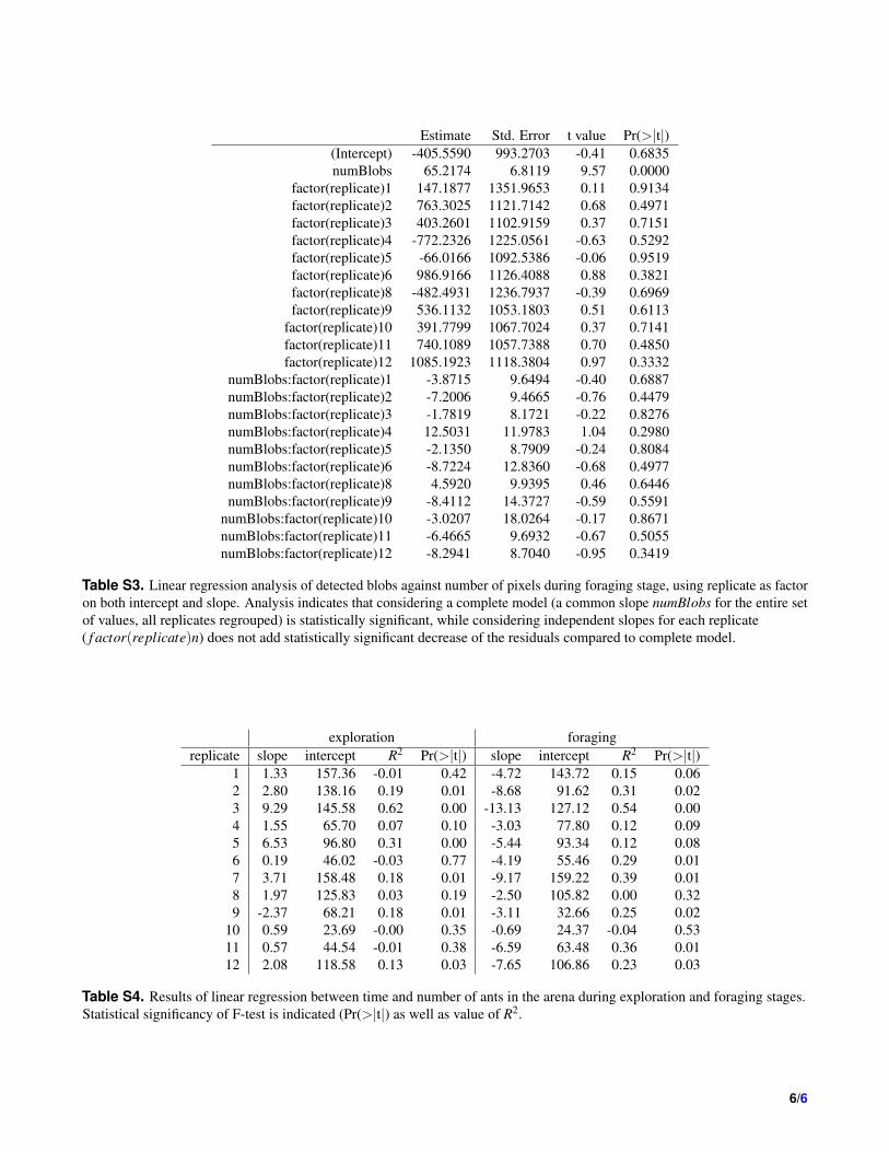
Table S3. Linear regression analysis of detected blobs against number of pixels during foraging stage, using replicate as factoron both intercept and slope. Analysis indicates that considering a complete model (a common slope numBlobs for the entire setof values, all replicates regrouped) is statistically significant, while considering independent slopes for each replicate( f actor(replicate)n) does not add statistically significant decrease of the residuals compared to complete model.

exploration foragingreplicate slope intercept R2 Pr(>|t|) slope intercept R2 Pr(>|t|)

1 1.33 157.36 -0.01 0.42 -4.72 143.72 0.15 0.062 2.80 138.16 0.19 0.01 -8.68 91.62 0.31 0.023 9.29 145.58 0.62 0.00 -13.13 127.12 0.54 0.004 1.55 65.70 0.07 0.10 -3.03 77.80 0.12 0.095 6.53 96.80 0.31 0.00 -5.44 93.34 0.12 0.086 0.19 46.02 -0.03 0.77 -4.19 55.46 0.29 0.017 3.71 158.48 0.18 0.01 -9.17 159.22 0.39 0.018 1.97 125.83 0.03 0.19 -2.50 105.82 0.00 0.329 -2.37 68.21 0.18 0.01 -3.11 32.66 0.25 0.02

10 0.59 23.69 -0.00 0.35 -0.69 24.37 -0.04 0.5311 0.57 44.54 -0.01 0.38 -6.59 63.48 0.36 0.0112 2.08 118.58 0.13 0.03 -7.65 106.86 0.23 0.03

Table S4. Results of linear regression between time and number of ants in the arena during exploration and foraging stages.Statistical significancy of F-test is indicated (Pr(>|t|) as well as value of R2.

6/6