an augmented lagrangian approach to constrained map inference
TRANSCRIPT
An Augmented Lagrangian Approach to Constrained MAP Inference
Andre F. T. Martins†‡ [email protected] A. T. Figueiredo‡ [email protected] M. Q. Aguiar] [email protected] A. Smith† [email protected] P. Xing† [email protected]†School of Computer Science, Carnegie Mellon University, Pittsburgh, PA, USA‡Instituto de Telecomunicacoes / ]Instituto de Sistemas e Robotica, Instituto Superior Tecnico, Lisboa, Portugal
Abstract
We propose a new algorithm for approximateMAP inference on factor graphs, by combin-ing augmented Lagrangian optimization withthe dual decomposition method. Each slavesubproblem is given a quadratic penalty,which pushes toward faster consensus than inprevious subgradient approaches. Our algo-rithm is provably convergent, parallelizable,and suitable for fine decompositions of thegraph. We show how it can efficiently han-dle problems with (possibly global) structuralconstraints via simple sort operations. Ex-periments on synthetic and real-world datashow that our approach compares favorablywith the state-of-the-art.
1. Introduction
Graphical models enable compact representations ofprobability distributions, being widely used in com-puter vision, natural language processing (NLP), andcomputational biology (Koller & Friedman, 2009). Aprevalent problem is the one of inferring the most prob-able configuration, the so-called maximum a posteriori(MAP). Unfortunately, this problem is intractable, ex-cept for a limited class of models. This fact precludescomputing the MAP exactly in many important mod-els involving non-local features or requiring structuralconstraints to ensure valid predictions.
A significant body of research has thus been placed onapproximate MAP inference, e.g., via linear program-ming relaxations (Schlesinger, 1976). Several message-passing algorithms have been proposed that exploit
Appearing in Proceedings of the 28 th International Con-ference on Machine Learning, Bellevue, WA, USA, 2011.Copyright 2011 by the author(s)/owner(s).
the graph structure in these relaxations (Wainwrightet al., 2005; Kolmogorov, 2006; Werner, 2007; Glober-son & Jaakkola, 2008; Ravikumar et al., 2010). In thesame line, Komodakis et al. (2007) proposed a methodbased on the classical dual decomposition technique(DD; Dantzig & Wolfe 1960; Everett III 1963; Shor1985), which breaks the original problem into a setof smaller (slave) subproblems, splits the shared vari-ables, and tackles the Lagrange dual with the subgra-dient algorithm. Initially applied in computer vision,DD has also been shown effective in NLP (Koo et al.,2010). The drawback is that the subgradient algorithmis very slow to converge when the number of slaves islarge. This led Jojic et al. (2010) to propose an accel-erated gradient method by smoothing the objective.
In this paper, we ally the simplicity of DD withthe effectiveness of augmented Lagrangian methods,which have a long-standing history in optimization(Hestenes, 1969; Powell, 1969; Glowinski & Marroco,1975; Gabay & Mercier, 1976; Boyd et al., 2011). Theresult is a novel algorithm for approximate MAP infer-ence: DD-ADMM (Dual Decomposition with the Al-ternating Direction Method of Multipliers). Ratherthan placing all efforts in attempting progress inthe dual, DD-ADMM looks for a saddle point ofthe Lagrangian function, which is augmented with aquadratic term to penalize slave disagreements. Keyfeatures of DD-ADMM are:
• It is suitable for heavy parallelization (many slaves);• it is provably convergent, even when each slave sub-
problem is only solved approximately;• consensus among slaves is fast, by virtue of the
quadratic penalty term, hence it exhibits faster con-vergence in the primal than competing methods;
• in addition to providing an optimality certificate forthe exact MAP, it also provides guarantees that theLP-relaxed solution has been found.
An Augmented Lagrangian Approach to Constrained MAP Inference
After providing the necessary background (Sect. 2)and introducing and analyzing DD-ADMM (Sect. 3),we turn to the slave subproblems (Sect. 4). Of partic-ular concern to us are problems with structural con-straints, which arise commonly in NLP, vision, andother structured prediction tasks. We show that, forseveral important constraints, each slave can be solvedexactly and efficiently via sort operations. Experi-ments with pairwise MRFs and dependency parsing(Sect. 5) testify to the success of our approach.
2. Background
2.1. Problem Formulation
Let X , (X1, . . . , XN ) ∈ X be a vector of discreterandom variables, where each Xi ∈ Xi, with Xi a fi-nite set. We assume that X has a Gibbs distributionassociated with a factor graph G (Kschischang et al.,2001), composed of a set of variable nodes {1, . . . , N}and a set of factor nodes A, with each a ∈ A linked toa subset of variables N(a) ⊆ {1, . . . , N}:
Pθ,φ(x) ∝ exp(∑N
i=1 θi(xi) +∑a∈A φa(xa)
). (1)
Above, xa stands for the subvector indexed by the el-ements of N(a), and θi(.) and φa(.) are, respectively,unary and higher-order log-potential functions. To ac-commodate hard constraints, we allow these functionsto take values in R ∪ {−∞}. For simplicity, we writeθi , (θi(xi))xi∈Xi and φa , (φa(xa))xa∈Xa .
We are interested in the task of finding the most prob-able assignment (the MAP), x , arg maxx∈X Pθ,φ(x).This (in general NP-hard) combinatorial problem canbe transformed into a linear program (LP) by in-troducing marginal variables µ , (µi)ni=1 and ν ,(νa)a∈A, constrained to the marginal polytope of G,i.e., the set of realizable marginals (Wainwright & Jor-dan, 2008). Denoting this set by M(G), this yields
OPT , max(µ,ν)∈M(G)
∑i θ>i µi +
∑a φ>a νa, (2)
which always admits an integer solution. Unfortu-nately, M(G) often lacks a concise representation,which renders (2) intractable. A common workaroundis to replace M(G) by the outer bound L(G) ⊇M(G)—the so-called local polytope, defined as
L(G) =
(µ,ν)
∣∣∣∣∣ 1>µi = 1,∀i ∧Hiaνa = µi,∀a, i ∈ N(a) ∧νa ≥ 0,∀a
,
(3)where Hia(xi,xa) = 1 if [xa]i = xi, and 0 otherwise.This yields the following LP relaxation of (2):
OPT′ , max(µ,ν)∈L(G)
∑i θ>i µi +
∑a φ>a νa, (4)
which will be our main focus throughout. Obviously,OPT′ ≥ OPT, since L(G) ⊇M(G).
2.2. Dual Decomposition
Several message passing algorithms (Wainwright et al.,2005; Kolmogorov, 2006; Globerson & Jaakkola, 2008)are derived via some reformulation of (4) followed bydualization. The DD method (Komodakis et al., 2007)reformulates (4) by adding new variables νai (for eachfactor a and i ∈ N(a)) that are local “replicas” ofthe marginals µi. Letting N(i) , {a|i ∈ N(a)} anddi = |N(i)| (the degree of node i), (4) is rewritten as
maxν,µ
∑a
(∑i∈N(a) d
−1i θ
>i ν
ai + φ>a νa
)(5)
s.t. (νaN(a),νa) ∈M(Ga), ∀aνai = µi, ∀a, i ∈ N(a),
where Ga is the subgraph of G comprised only offactor a and the variables in N(a), M(Ga) is thecorresponding marginal polytope, and we denoteνaN(a) , (νai )i∈N(a). (Note that by definition, L(G) ={(µ,ν) | (µNa
,νa) ∈ M(Ga), ∀a ∈ A}.) Problem (5)would be completely separable (over the factors) if itwere not the “coupling” constraints νai = µi. Intro-ducing Lagrange multipliers λai for these constraints,the dual problem (master) becomes
minλ
L(λ) ,∑a sa
((d−1i θi + λai
)i∈N(a)
,φa
)s.t. λ ∈ Λ ,
{λ∣∣ ∑
a∈N(i) λai = 0, ∀i
}, (6)
where each sa corresponds to a slave subproblem
sa(ωaN(a),φa) , max(νa
N(a),νa)
∈M(Ga)
∑i∈N(a)
ω>i νai + φ>a νa. (7)
Note that the slaves (7) are MAP problems of the samekind as (2), but local to each factor a. Denote by(νaN(a), νa) = map(ωaN(a),φa) the maximizer of (7).The master problem (6) can be addressed elegantlywith a projected subgradient algorithm: note that asubgradient ∇λa
iL(λ) is readily available upon solving
the ath slave, via ∇λaiL(λ) = νai . These slaves can
be handled in parallel and then have their solutionsgathered for computing a projection onto Λ, which issimply a centering operation. This results in Alg. 1.
Alg. 1 inherits the properties of subgradient algo-rithms, hence it converges to the optimal value ofOPT′ in (4) if the stepsize sequence (ηt)t∈T is dimin-ishing and nonsummable (Bertsekas et al., 1999). Inpractice, convergence can be quite slow if the numberof slaves is large. This is because it may be hard toreach a consensus on variables with many replicas.
An Augmented Lagrangian Approach to Constrained MAP Inference
Algorithm 1 DD-Subgradient1: input: factor graph G, parameters θ,φ, number of
iterations T , stepsize sequence (ηt)Tt=1
2: Initialize λ = 03: for t = 1 to T do4: for each factor a ∈ A do5: Set ωai = d−1
i θi + λai , for i ∈ N(a)6: Compute (νaN(a), νa) = map
`ωaN(a),φa
´7: end for8: Compute average µi = di
−1Pa:i∈N(a) ν
ai
9: Update λai ← λai − ηt (νai − µi)10: end for
11: output: λ
3. Augmented Lagrangian Method
In this section we introduce a faster method, DD-ADMM, which replaces the MAP computation ateach factor a by a (usually simple) quadratic prob-lem (QP); this method penalizes disagreements amongslaves more aggressively than the subgradient method.
Given an optimization problem with equality con-straints, the augmented Lagrangian (AL) function isthe Lagrangian augmented with a quadratic constraintviolation penalty. For the constraint problem (5), it is
Aη(µ,ν,λ) ,∑a
( ∑i∈N(a)
(d−1i θi + λai
)>νai + φ>a νa
)−∑a
∑i∈N(a)
λai>µi −
η
2
∑a
∑i∈N(a)
‖νai − µi‖2, (8)
where η controls the weight of the penalty. Appliedto our problem, a traditional AL method (Hestenes,1969; Powell, 1969) would alternate between the jointmaximization of Aη(µ,ν,λ) w.r.t. µ and ν, and an up-date of the Lagrange multipliers λ. Unfortunately, thequadratic term in (8) breaks the separability, makingthe joint maximization w.r.t. µ and ν unappealing.
We bypass this problem by using the alternating direc-tion method of multipliers (ADMM; Gabay & Mercier1976; Glowinski & Marroco 1975), in which the jointmaximization is replaced by a single Gauss-Seidel step.This yields the following updates:
ν(t) ← argmaxν
Aηt(µ(t−1),ν,λ(t−1)), (9)
µ(t) ← argmaxµ
Aηt(µ,ν(t),λ(t−1)), (10)
λa(t)i ← λ
a(t−1)i − τηt
(νa(t)i − µ
(t)i
),∀a, i ∈ N(a). (11)
Crucially, the maximization w.r.t. µ (10) has a closedform, while that w.r.t. ν (9) can be carried out inparallel at each factor, as in Alg. 1. The only differenceis that, instead of computing the MAP, each slave now
Algorithm 2 DD-ADMM1: input: factor graph G, parameters θ,φ, number of
iterations T , sequence (ηt)Tt=1, parameter τ
2: Initialize µ uniformly, λ = 03: for t = 1 to T do4: for each factor a ∈ A do5: Set ωai = d−1
i θi + λai + ηtµi, for i ∈ N(a)6: Update (νaN(a),νa)← quadηt
`ωaN(a),φa
´7: end for8: Update µi ← di
−1Pa:i∈N(a)
`νai − η−1
t λai´
9: Update λai ← λai − τηt (νai − µi)10: end for
11: output: µ,ν,λ
needs to solve a QP of the form
min(νa
N(a),νa)∈M(Ga)
ηt2
∑i∈N(a)
‖νai − η−1t ωai ‖2 − φ
>a νa. (12)
The resulting algorithm is DD-ADMM (Alg. 2). Letquadηt
(ωN(a),φa) denote the solution of (12); as ηt →0, quadηt
(ωN(a),φa) approaches map(ωN(a),φa),hence Alg. 2 approaches Alg. 1. However, DD-ADMMconverges without the need of decreasing ηt:
Proposition 1 Let (µ(t),ν(t),λ(t))t be the sequenceof iterates produced by Alg. 2 with a fixed ηt = η and0 < τ ≤ (
√5 + 1)/2 ' 1.61. Then the following holds:
1. Primal feasibility of (5) is achieved in the limit,i.e., ‖νa(t)i − µ(t)
i ‖ → 0,∀a ∈ A, i ∈ N(a);
2. (µ(t),ν(t)) converges to an optimal solution of (4);
3. λ(t) converges to an optimal solution of (6);
4. λ(t) is always dual feasible; hence the objective of(6) evaluated at λ(t) approaches OPT′ from above.
Proof: 1, 2, and 3 are general properties of ADMM al-gorithms (Glowinski & Le Tallec, 1989, Thm. 4.2). Allnecessary conditions are met: problem (5) is convexand the coupling constraint can be written in the form(νaN(a))a∈A = Mµ where M has full column rank. To
show 4, use induction: λ(0) = 0 ∈ Λ; if λ(t−1) ∈ Λ,i.e.,
∑a∈N(i) λ
a(t−1)i = 0, ∀i, then, after line 9,
∑a∈N(i)
λa(t)i =
∑a∈N(i)
λa(t−1)i − τηt
∑a∈N(i)
νa(t)i − diµ(t)
i
= (1− τ)
∑a∈N(i)
λa(t−1)i = 0 ⇒ λ(t) ∈ Λ. �
Prop. 1 reveals yet another important feature of DD-ADMM: after a sufficient decrease of the residual term,

An Augmented Lagrangian Approach to Constrained MAP Inference
say∑a
∑i∈N(a) ‖νai − µi‖2 < ε, we have at hand a ε-
feasible primal-dual pair. If, in addition, the dualitygap (difference between (4) and (6)) is < δ, then weare in possession of an (ε, δ)-optimality certificate forthe LP relaxation. Such a certificate is not readilyavailable in Alg. 1, unless the relaxation is tight.
The next proposition, based on results of Eckstein& Bertsekas (1992), states that convergence may stillhold if (12) is solved approximately.
Proposition 2 Let ηt = η be fixed and τ = 1. Con-sider the sequence of residuals r(t) , (r(t)a )a∈A, where
r(t)a , ‖(νa(t)N(a),ν
(t)a )− quadηt
(ω(t)N(a),φa)‖.
Then, Prop. 1 still holds provided∑∞t=1 ‖r(t)‖ <∞.
4. Solving the Slave Subproblems
We next show how to efficiently solve (12). Severalcases admit closed-form solutions: binary pairwise fac-tors, some factors expressing hard constraints, and fac-tors linked to multi-valued variables, once binarized.In all cases, the asymptotic computational cost is thesame as that of MAP computations, up to a logarith-mic factor. Detailed proofs of the following facts areincluded as supplementary material.
4.1. Binary pairwise factors
If factor a is binary and pairwise (|N(a)| = 2), problem(12) can be re-written as the minimization of 1
2 (z1 −c1)2 + 1
2 (z2− c2)2− c12z12, w.r.t. (z1, z2, z12) ∈ [0, 1]3,under the constraints z12 ≤ z1, z12 ≤ z2, and z12 ≥z1+z2−1, where c1, c2 and c12 are functions of ωai andφa. Considering c12 ≥ 0, without loss of generality (ifc12 < 0, we recover this case by redefining c′1 = c1+c12,c′2 = 1 − c2, c′12 = −c12, z′2 = 1 − z2, z′12 = z1 − z12),the lower bound constraints z12 ≥ z1 + z2 − 1 andz12 ≥ 0 are always innactive and can be ignored. Byinspecting the KKT conditions we obtain the followingclosed-form solution: z∗12 = min{z∗1 , z∗2} and
(z∗1 , z∗2) =
([c1]U, [c2 + c12]U) if c1 > c2 + c12([c1 + c12]U, [c2]U) if c2 > c1 + c12([(c1 + c2 + c12)/2]U ,[(c1 + c2 + c12)/2]U) otherwise,
where [x]U = min{max{x, 0}, 1} denotes the projec-tion (clipping) onto the unit interval.
4.2. Hard constraint factors
Many applications, e.g., in error-correcting coding(Richardson & Urbanke, 2008) and NLP (Smith & Eis-ner, 2008; Martins et al., 2010; Tarlow et al., 2010)
involve hard constraint factors—these are factors withindicator log-potential functions: φa(xa) = 0, if xa ∈Sa, and −∞ otherwise, where Sa is an acceptance set.For binary variables, these factors impose logical con-straints; e.g.,
• the one-hot xor factor, for which Sxor ={(x1, . . . , xn) ∈ {0, 1}n|
∑ni=1 xi = 1},
• the or factor, for which Sor = {(x1, . . . , xn) ∈{0, 1}n|
∨ni=1 xi = 1},
• the or-with-output factor, for which Sor-out ={(x1, . . . , xn) ∈ {0, 1}n|
∨n−1i=1 xi = xn}.
Variants of these factors (e.g., with negated in-puts/outputs) allow computing a wide range of otherlogical functions. It can be shown that the marginalpolytope of a hard factor with binary variables andacceptance set Sa is defined by z ∈ conv Sa, wherez , (µ1(1), . . . , µn(1)) and conv denotes the convexhull. Letting c , (ωia(1) + 1 − ωia(0))i∈N(a), problem(12) is that of minimizing ‖z − c‖2 s.t. z ∈ conv Sa,which is a Euclidean projection onto a polyhedron:
• conv Sxor is the probability simplex; the projectionis efficiently obtained via a sort (Duchi et al., 2008).
• conv Sor is a “faulty” hypercube with a vertex re-moved, and conv Sor-out is a pyramid whose base is ahypercube with a vertex removed; both projectionscan be efficiently computed with sort operations.
The algorithms and proofs of correctness are providedas supplementary material. In all cases, complexity isO(|N(a)| log |N(a)|) and can be improved to O(|N(a)|)using a technique similar to Duchi et al. (2008).
4.3. Larger slaves and multi-valued variables
For general factors, a closed-form solution of problem(12) is not readily available. One possible strategy (ex-ploiting Prop. 2) is to use an inexact algorithm thatbecomes sufficiently accurate as Alg. 2 proceeds; thiscan be achieved by warm-starting with the solution ob-tained in the previous iteration. This strategy can beuseful for handling coarser decompositions, in whicheach factor is a subgraph such as a chain or a tree.However, unlike the map problem in DD-subgradient,in which dynamic programming can be used to com-pute an exact solution for these special structures, thatdoes not seem possible in quad.
Yet, there is an alternative strategy for handling multi-valued variables, which is to binarize the graph andmake use of the results established in Sect. 4.2 for hardconstraint factors. We illustrate this procedure forpairwise MRFs (but the idea carries over when higherorder potentials are used): let X1, . . . , XN be the vari-ables of the original graph, and E ⊆ {1, . . . , N}2 be
An Augmented Lagrangian Approach to Constrained MAP Inference
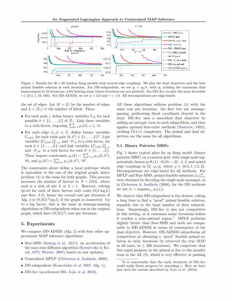
Figure 1. Results for 30× 30 random Ising models with several edge couplings. We plot the dual objectives and the bestprimal feasible solution at each iteration. For DD-subgradient, we set ηt = η0/t, with η0 yielding the maximum dualimprovement in 10 iterations, with halving steps (those iterations are not plotted). For DD-Acc we plot the most favorableε ∈ {0.1, 1, 10, 100}. For DD-ADMM, we set η = 5.0 and τ = 1.0. All decompositions are edge-based.
the set of edges. Let M = |E| be the number of edgesand L = |Xi|,∀i the number of labels. Then:
• For each node i, define binary variables Uik for eachpossible k ∈ {1, . . . , L} of Xi. Link these variablesto a xor factor, imposing
∑Lk=1 µi(k) = 1, ∀i.
• For each edge (i, j) ∈ E, define binary variablesUijkk′ for each value pair (k, k′) ∈ {1, . . . , L}2. Linkvariables {Uijkk′}Lk′=1 and ¬Uik to a xor factor, foreach k ∈ {1, . . . , L}; and link variables {Uijkk′}Lk=1
and ¬Ujk′ to a xor factor for each k′ ∈ {1, . . . , L}.These impose constraints µi(k) =
∑Lk′=1 µij(k, k
′),∀k, and µj(k′) =
∑lk=1 µij(k, k
′), ∀k′.
The constraints above define a local polytope whichis equivalent to the one of the original graph, henceproblem (4) is the same for both graphs. This processincreases the number of factors to N + 2ML, whereeach is a xor of size L or L + 1. However, solvingquad for each of these factors only costs O(L logL)(see Sect. 4.2), hence the overall cost per iteration ofAlg. 2 is O(ML2 logL) if the graph is connected. Upto a log factor, this is the same as message-passingalgorithms or DD-subgradient when run in the originalgraph, which have O(ML2) cost per iteration.
5. Experiments
We compare DD-ADMM (Alg. 2) with four other ap-proximate MAP inference algorithms:
• Star-MSD (Sontag et al., 2011), an acceleration ofthe max-sum diffusion algorithm (Kovalevsky & Ko-val, 1975; Werner, 2007) based on star updates;
• Generalized MPLP (Globerson & Jaakkola, 2008);
• DD-subgradient (Komodakis et al. 2007, Alg. 1);
• DD-Acc (accelerated DD, Jojic et al. 2010).
All these algorithms address problem (4) with thesame cost per iteration: the first two use message-passing, performing block coordinate descent in thedual; DD-Acc uses a smoothed dual objective byadding an entropic term to each subproblem, and thenapplies optimal first-order methods (Nesterov, 1983),yielding O(1/ε) complexity. The primal and dual ob-jectives are the same for all algorithms.
5.1. Binary Pairwise MRFs
Fig. 1 shows typical plots for an Ising model (binarypairwise MRF) on a random grid, with single node log-potentials chosen as θi(1)−θi(0) ∼ U[−1, 1] and mixededge couplings in U[−ρ, ρ], where ρ ∈ {0.5, 1, 1.5, 2}.Decompositions are edge-based for all methods. ForMPLP and Star-MSD, primal feasible solutions (xi)Ni=1
were obtained by decoding the single node messages, asin Globerson & Jaakkola (2008); for the DD methodswe use xi = argmaxxi
µi(xi).
We observe that DD-subgradient is the slowest, takinga long time to find a “good” primal feasible solution,arguably due to the large number of slave subprob-lems. Surprisingly, DD-Acc is also not competitivein this setting, as it consumes many iterations beforeit reaches a near-optimal region.1 MPLP performsslightly better than Star-MSD and both are compa-rable to DD-ADMM in terms of convergence of thedual objective. However, DD-ADMM outperforms allcompetitors at obtaining a “good” feasible primal so-lution in early iterations (it retrieved the true MAPin all cases, in ≤ 200 iterations). We conjecture thatthis rapid progress in the primal is due to the penaltyterm in the AL (8), which is very effective at pushing
1It is conceivable that the early iterations of DD-Acccould make faster progress by annealing ε. Here we havejust used the variant described by Jojic et al. (2010).
An Augmented Lagrangian Approach to Constrained MAP Inference
0 200 400 600 800 1000
2005
2010
2015
2020
2025
Number of Iterations
Dua
l Obj
ectiv
e
MPLPDD−AccDD−ADMMDual Opt.
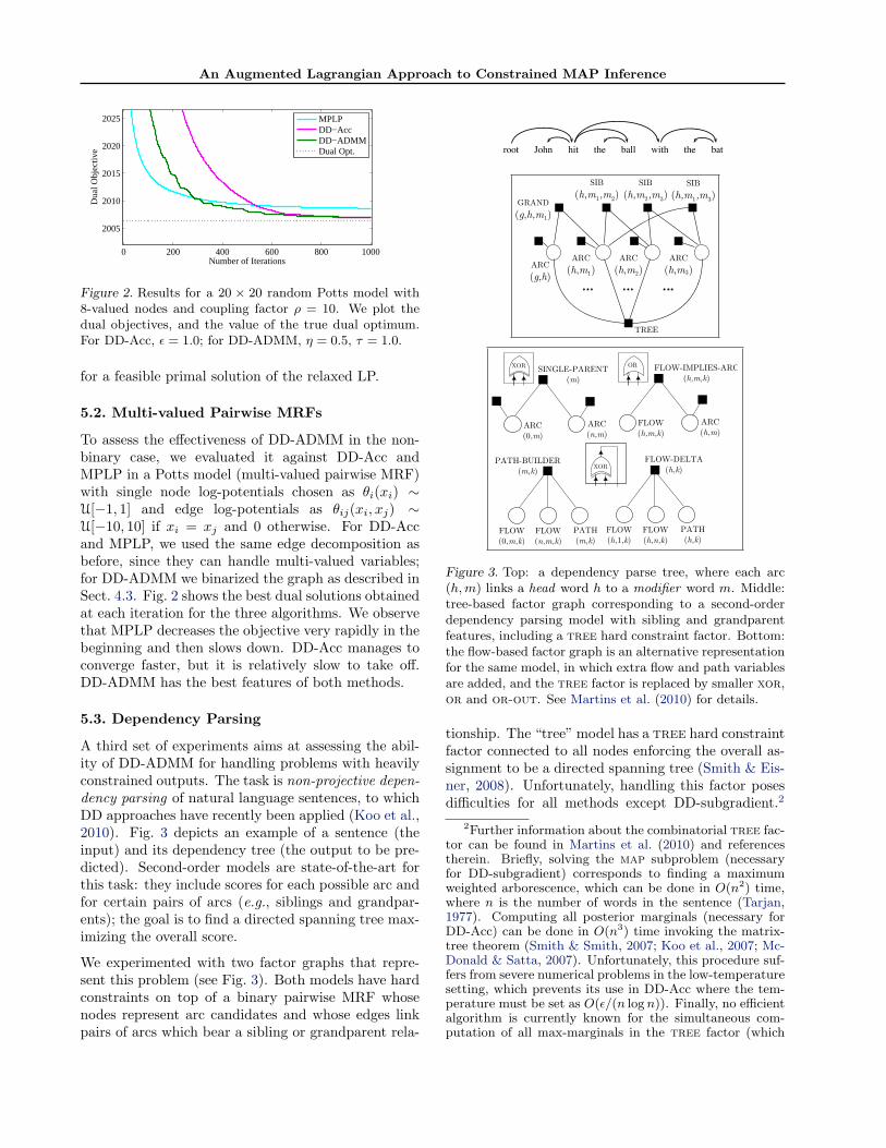
Figure 2. Results for a 20 × 20 random Potts model with8-valued nodes and coupling factor ρ = 10. We plot thedual objectives, and the value of the true dual optimum.For DD-Acc, ε = 1.0; for DD-ADMM, η = 0.5, τ = 1.0.
for a feasible primal solution of the relaxed LP.
5.2. Multi-valued Pairwise MRFs
To assess the effectiveness of DD-ADMM in the non-binary case, we evaluated it against DD-Acc andMPLP in a Potts model (multi-valued pairwise MRF)with single node log-potentials chosen as θi(xi) ∼U[−1, 1] and edge log-potentials as θij(xi, xj) ∼U[−10, 10] if xi = xj and 0 otherwise. For DD-Accand MPLP, we used the same edge decomposition asbefore, since they can handle multi-valued variables;for DD-ADMM we binarized the graph as described inSect. 4.3. Fig. 2 shows the best dual solutions obtainedat each iteration for the three algorithms. We observethat MPLP decreases the objective very rapidly in thebeginning and then slows down. DD-Acc manages toconverge faster, but it is relatively slow to take off.DD-ADMM has the best features of both methods.
5.3. Dependency Parsing
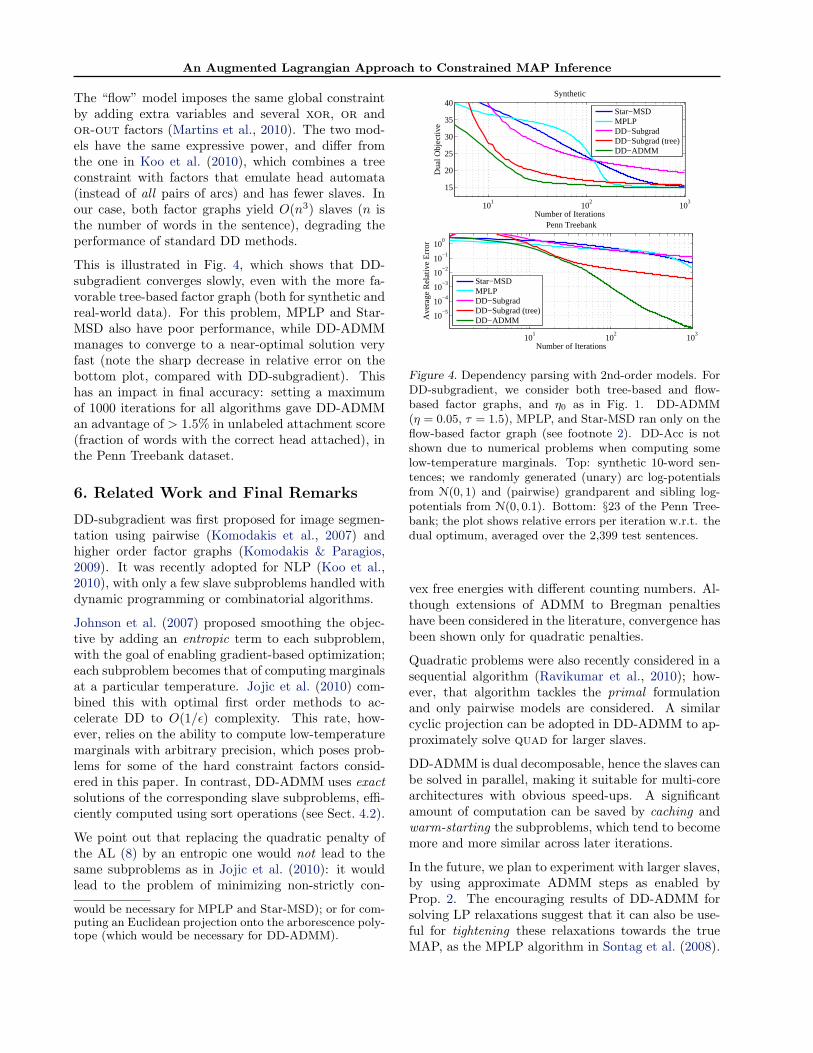
A third set of experiments aims at assessing the abil-ity of DD-ADMM for handling problems with heavilyconstrained outputs. The task is non-projective depen-dency parsing of natural language sentences, to whichDD approaches have recently been applied (Koo et al.,2010). Fig. 3 depicts an example of a sentence (theinput) and its dependency tree (the output to be pre-dicted). Second-order models are state-of-the-art forthis task: they include scores for each possible arc andfor certain pairs of arcs (e.g., siblings and grandpar-ents); the goal is to find a directed spanning tree max-imizing the overall score.
We experimented with two factor graphs that repre-sent this problem (see Fig. 3). Both models have hardconstraints on top of a binary pairwise MRF whosenodes represent arc candidates and whose edges linkpairs of arcs which bear a sibling or grandparent rela-
Non-projective Dependency Parsing using Spanning Tree Algorithms
Ryan McDonald Fernando Pereira
Department of Computer and Information Science
University of Pennsylvania
{ryantm,pereira}@cis.upenn.edu
Kiril Ribarov Jan Hajic
Institute of Formal and Applied Linguistics
Charles University
{ribarov,hajic}@ufal.ms.mff.cuni.cz
Abstract
We formalize weighted dependency pars-
ing as searching for maximum spanning
trees (MSTs) in directed graphs. Using
this representation, the parsing algorithm
of Eisner (1996) is sufficient for search-
ing over all projective trees inO(n3) time.More surprisingly, the representation is
extended naturally to non-projective pars-
ing using Chu-Liu-Edmonds (Chu and
Liu, 1965; Edmonds, 1967) MST al-
gorithm, yielding an O(n2) parsing al-gorithm. We evaluate these methods
on the Prague Dependency Treebank us-
ing online large-margin learning tech-
niques (Crammer et al., 2003; McDonald
et al., 2005) and show that MST parsing
increases efficiency and accuracy for lan-
guages with non-projective dependencies.
1 Introduction
Dependency parsing has seen a surge of inter-
est lately for applications such as relation extrac-
tion (Culotta and Sorensen, 2004), machine trans-
lation (Ding and Palmer, 2005), synonym genera-
tion (Shinyama et al., 2002), and lexical resource
augmentation (Snow et al., 2004). The primary
reasons for using dependency structures instead of
more informative lexicalized phrase structures is
that they are more efficient to learn and parse while
still encoding much of the predicate-argument infor-
mation needed in applications.
root John hit the ball with the bat
Figure 1: An example dependency tree.
Dependency representations, which link words to
their arguments, have a long history (Hudson, 1984).
Figure 1 shows a dependency tree for the sentence
John hit the ball with the bat. We restrict ourselves
to dependency tree analyses, in which each word de-
pends on exactly one parent, either another word or a
dummy root symbol as shown in the figure. The tree
in Figure 1 is projective, meaning that if we put the
words in their linear order, preceded by the root, the
edges can be drawn above the words without cross-
ings, or, equivalently, a word and its descendants
form a contiguous substring of the sentence.
In English, projective trees are sufficient to ana-
lyze most sentence types. In fact, the largest source
of English dependency trees is automatically gener-
ated from the Penn Treebank (Marcus et al., 1993)
and is by convention exclusively projective. How-
ever, there are certain examples in which a non-
projective tree is preferable. Consider the sentence
John saw a dog yesterday which was a Yorkshire Ter-
rier. Here the relative clause which was a Yorkshire
Terrier and the object it modifies (the dog) are sep-
arated by an adverb. There is no way to draw the
dependency tree for this sentence in the plane with
no crossing edges, as illustrated in Figure 2. In lan-
guages with more flexible word order than English,
such as German, Dutch and Czech, non-projective
dependencies are more frequent. Rich inflection
systems reduce reliance on word order to express
TREE
1
ARC
(h,m�)
SIB
(h,m�,m�)1 2
SIB
(h,m�,m�)1 3
SIB
(h,m�,m�)2 3GRAND
(g,h,m�)1
2
ARC
(h,m�) 3
ARC
(h,m�)ARC
(g,h)
FLOW
(0,m,k)
FLOW
(n,m,k)
PATH
(m,k)
PATH-BUILDER
(m,k)
FLOW
(h,1,k)
FLOW
(h,n,k)
PATH
(h,k)
FLOW-DELTA
(h,k)
ARC
(h,m)FLOW(h,m,k)
FLOW-IMPLIES-ARC
(h,m,k)
ARC
(0,m)
ARC(n,m)
SINGLE-PARENT
(m)
XOR
XOR
OR
Figure 3. Top: a dependency parse tree, where each arc(h,m) links a head word h to a modifier word m. Middle:tree-based factor graph corresponding to a second-orderdependency parsing model with sibling and grandparentfeatures, including a tree hard constraint factor. Bottom:the flow-based factor graph is an alternative representationfor the same model, in which extra flow and path variablesare added, and the tree factor is replaced by smaller xor,or and or-out. See Martins et al. (2010) for details.
tionship. The “tree” model has a tree hard constraintfactor connected to all nodes enforcing the overall as-signment to be a directed spanning tree (Smith & Eis-ner, 2008). Unfortunately, handling this factor posesdifficulties for all methods except DD-subgradient.2
2Further information about the combinatorial tree fac-tor can be found in Martins et al. (2010) and referencestherein. Briefly, solving the map subproblem (necessaryfor DD-subgradient) corresponds to finding a maximumweighted arborescence, which can be done in O(n2) time,where n is the number of words in the sentence (Tarjan,1977). Computing all posterior marginals (necessary forDD-Acc) can be done in O(n3) time invoking the matrix-tree theorem (Smith & Smith, 2007; Koo et al., 2007; Mc-Donald & Satta, 2007). Unfortunately, this procedure suf-fers from severe numerical problems in the low-temperaturesetting, which prevents its use in DD-Acc where the tem-perature must be set as O(ε/(n logn)). Finally, no efficientalgorithm is currently known for the simultaneous com-putation of all max-marginals in the tree factor (which
An Augmented Lagrangian Approach to Constrained MAP Inference
The “flow” model imposes the same global constraintby adding extra variables and several xor, or andor-out factors (Martins et al., 2010). The two mod-els have the same expressive power, and differ fromthe one in Koo et al. (2010), which combines a treeconstraint with factors that emulate head automata(instead of all pairs of arcs) and has fewer slaves. Inour case, both factor graphs yield O(n3) slaves (n isthe number of words in the sentence), degrading theperformance of standard DD methods.
This is illustrated in Fig. 4, which shows that DD-subgradient converges slowly, even with the more fa-vorable tree-based factor graph (both for synthetic andreal-world data). For this problem, MPLP and Star-MSD also have poor performance, while DD-ADMMmanages to converge to a near-optimal solution veryfast (note the sharp decrease in relative error on thebottom plot, compared with DD-subgradient). Thishas an impact in final accuracy: setting a maximumof 1000 iterations for all algorithms gave DD-ADMMan advantage of > 1.5% in unlabeled attachment score(fraction of words with the correct head attached), inthe Penn Treebank dataset.
6. Related Work and Final Remarks
DD-subgradient was first proposed for image segmen-tation using pairwise (Komodakis et al., 2007) andhigher order factor graphs (Komodakis & Paragios,2009). It was recently adopted for NLP (Koo et al.,2010), with only a few slave subproblems handled withdynamic programming or combinatorial algorithms.
Johnson et al. (2007) proposed smoothing the objec-tive by adding an entropic term to each subproblem,with the goal of enabling gradient-based optimization;each subproblem becomes that of computing marginalsat a particular temperature. Jojic et al. (2010) com-bined this with optimal first order methods to ac-celerate DD to O(1/ε) complexity. This rate, how-ever, relies on the ability to compute low-temperaturemarginals with arbitrary precision, which poses prob-lems for some of the hard constraint factors consid-ered in this paper. In contrast, DD-ADMM uses exactsolutions of the corresponding slave subproblems, effi-ciently computed using sort operations (see Sect. 4.2).
We point out that replacing the quadratic penalty ofthe AL (8) by an entropic one would not lead to thesame subproblems as in Jojic et al. (2010): it wouldlead to the problem of minimizing non-strictly con-
would be necessary for MPLP and Star-MSD); or for com-puting an Euclidean projection onto the arborescence poly-tope (which would be necessary for DD-ADMM).
101
102
103
15
20
25
30
35
40
Number of Iterations
Dua
l Obj
ectiv
e
Synthetic
Star−MSDMPLPDD−SubgradDD−Subgrad (tree)DD−ADMM
101
102
103
100
10−1
10−2
10−3
10−4
10−5
Number of Iterations
Ave
rage
Rel
ativ
e E
rror
Penn Treebank
Star−MSDMPLPDD−SubgradDD−Subgrad (tree)DD−ADMM
Figure 4. Dependency parsing with 2nd-order models. ForDD-subgradient, we consider both tree-based and flow-based factor graphs, and η0 as in Fig. 1. DD-ADMM(η = 0.05, τ = 1.5), MPLP, and Star-MSD ran only on theflow-based factor graph (see footnote 2). DD-Acc is notshown due to numerical problems when computing somelow-temperature marginals. Top: synthetic 10-word sen-tences; we randomly generated (unary) arc log-potentialsfrom N(0, 1) and (pairwise) grandparent and sibling log-potentials from N(0, 0.1). Bottom: §23 of the Penn Tree-bank; the plot shows relative errors per iteration w.r.t. thedual optimum, averaged over the 2,399 test sentences.
vex free energies with different counting numbers. Al-though extensions of ADMM to Bregman penaltieshave been considered in the literature, convergence hasbeen shown only for quadratic penalties.
Quadratic problems were also recently considered in asequential algorithm (Ravikumar et al., 2010); how-ever, that algorithm tackles the primal formulationand only pairwise models are considered. A similarcyclic projection can be adopted in DD-ADMM to ap-proximately solve quad for larger slaves.
DD-ADMM is dual decomposable, hence the slaves canbe solved in parallel, making it suitable for multi-corearchitectures with obvious speed-ups. A significantamount of computation can be saved by caching andwarm-starting the subproblems, which tend to becomemore and more similar across later iterations.
In the future, we plan to experiment with larger slaves,by using approximate ADMM steps as enabled byProp. 2. The encouraging results of DD-ADMM forsolving LP relaxations suggest that it can also be use-ful for tightening these relaxations towards the trueMAP, as the MPLP algorithm in Sontag et al. (2008).

An Augmented Lagrangian Approach to Constrained MAP Inference
AcknowledgmentsA. M. was supported by a FCT/ICTI grant through the
CMU-Portugal Program, and also by Priberam. This work
was partially supported by the FET programme (EU FP7),
under the SIMBAD project (contract 213250), and by a
FCT grant PTDC/EEA-TEL/72572/2006. N. S. was sup-
ported by NSF CAREER IIS-1054319. E. X. was sup-
ported by AFOSR FA9550010247, ONR N000140910758,
NSF CAREER DBI-0546594, NSF IIS-0713379, and an Al-
fred P. Sloan Fellowship.
References
Bertsekas, D., Hager, W., and Mangasarian, O. Nonlinearprogramming. Athena Scientific, 1999.
Bertsekas, D.P., Nedic, A., and Ozdaglar, A.E. Convexanalysis and optimization. Athena Scientific, 2003.
Boyd, S., Parikh, N., Chu, E., Peleato, B., and Eckstein, J.Distributed Optimization and Statistical Learning via theAlternating Direction Method of Multipliers (to appear).Now Publishers, 2011.
Boyle, J.P. and Dykstra, R.L. A method for finding pro-jections onto the intersections of convex sets in Hilbertspaces. In Advances in order restricted statistical infer-ence, pp. 28–47. Springer Verlag, 1986.
Dantzig, G. and Wolfe, P. Decomposition principle for lin-ear programs. Operations Research, 8(1):101–111, 1960.
Duchi, J., Shalev-Shwartz, S., Singer, Y., and Chandra, T.Efficient projections onto the L1-ball for learning in highdimensions. In ICML, 2008.
Eckstein, J. and Bertsekas, D. On the Douglas-Rachfordsplitting method and the proximal point algorithm formaximal monotone operators. Mathematical Program-ming, 55(1):293–318, 1992.
Everett III, H. Generalized Lagrange multiplier methodfor solving problems of optimum allocation of resources.Operations Research, 11(3):399–417, 1963.
Gabay, D. and Mercier, B. A dual algorithm for the solu-tion of nonlinear variational problems via finite elementapproximation. Computers and Mathematics with Ap-plications, 2(1):17–40, 1976.
Globerson, A. and Jaakkola, T. Fixing max-product:Convergent message passing algorithms for MAP LP-relaxations. NIPS, 20, 2008.
Glowinski, R. and Le Tallec, P. Augmented Lagrangianand operator-splitting methods in nonlinear mechanics.Society for Industrial Mathematics, 1989.
Glowinski, R. and Marroco, A. Sur l’approximation,par elements finis d’ordre un, et la resolution, parpenalisation-dualite, d’une classe de problemes deDirichlet non lineaires. Rev. Franc. Automat. Inform.Rech. Operat., 9:41–76, 1975.
Hestenes, M. Multiplier and gradient methods. Jour. Op-tim. Theory and Applic., 4:302–320, 1969.
Johnson, J.K., Malioutov, D.M., and Willsky, A.S. La-grangian relaxation for MAP estimation in graphicalmodels. In 45th Annual Allerton Conference on Com-munication, Control and Computing, 2007.
Jojic, V., Gould, S., and Koller, D. Accelerated dual de-composition for MAP inference. In ICML, 2010.
Koller, D. and Friedman, N. Probabilistic Graphical Mod-els: Principles and Techniques. The MIT Press, 2009.
Kolmogorov, V. Convergent tree-reweighted message pass-ing for energy minimization. IEEE Trans. Pattern Anal-ysis and Machine Intelligence, 28:1568–1583, 2006.
Komodakis, N. and Paragios, N. Beyond pairwise energies:Efficient optimization for higher-order MRFs. In CVPR,2009.
Komodakis, N., Paragios, N., and Tziritas, G. MRF op-timization via dual decomposition: Message-passing re-visited. In ICCV, 2007.
Koo, T., Globerson, A., Carreras, X., and Collins, M.Structured prediction models via the matrix-tree the-orem. In EMNLP, 2007.
Koo, T., Rush, A. M., Collins, M., Jaakkola, T., andSontag, D. Dual decomposition for parsing with non-projective head automata. In EMNLP, 2010.
Kovalevsky, V.A. and Koval, V.K. A diffusion algorithmfor decreasing energy of max-sum labeling problem.Glushkov Institute of Cybernetics, Kiev, USSR, 1975.
Kschischang, F. R., Frey, B. J., and Loeliger, H. A. Factorgraphs and the sum-product algorithm. IEEE Trans.Information Theory, 47, 2001.
Martins, A., Smith, N., Xing, E., Figueiredo, M., andAguiar, P. Turbo parsers: Dependency parsing by ap-proximate variational inference. In EMNLP, 2010.
McDonald, R. and Satta, G. On the complexity of non-projective data-driven dependency parsing. In IWPT,2007.
Nesterov, Y. A method of solving a convex programmingproblem with convergence rate O(1/k2). Soviet Math.Doklady, 27:372–376, 1983.
Powell, M. A method for nonlinear constraints in mini-mization problems. In Fletcher, R. (ed.), Optimization,pp. 283–298. Academic Press, 1969.
Ravikumar, P., Agarwal, A., and Wainwright, M. Message-passing for graph-structured linear programs: Proximalmethods and rounding schemes. JMLR, 11:1043–1080,2010.
Richardson, T.J. and Urbanke, R.L. Modern coding theory.Cambridge Univ Pr, 2008.
Schlesinger, M. Syntactic analysis of two-dimensional vi-sual signals in noisy conditions. Kibernetika, 4:113–130,1976.
Shor, N. Minimization methods for non-differentiable func-tions. Springer, 1985.
Smith, D. and Eisner, J. Dependency parsing by beliefpropagation. In EMNLP, 2008.
Smith, D. and Smith, N. Probabilistic models of nonpro-jective dependency trees. In EMNLP-CoNLL, 2007.
Sontag, D., Meltzer, T., Globerson, A., Weiss, Y., andJaakkola, T. Tightening LP relaxations for MAP usingmessage-passing. In UAI, 2008.
Sontag, D., Globerson, A., and Jaakkola, T. Introductionto dual decomposition for inference. In Optimization forMachine Learning. MIT Press, 2011.
Tarjan, R.E. Finding optimum branchings. Networks, 7(1):25–36, 1977.
Tarlow, D., Givoni, I. E., and Zemel, R. S. HOP-MAP:Efficient message passing with high order potentials. InAISTATS, 2010.
Wainwright, M. and Jordan, M. Graphical Models, Expo-nential Families, and Variational Inference. Now Pub-lishers, 2008.
Wainwright, M., Jaakkola, T., and Willsky, A. MAP es-timation via agreement on trees: message-passing andlinear programming. IEEE Trans. Information Theory,51(11):3697–3717, 2005.
Werner, T. A linear programming approach to max-sumproblem: A review. IEEE Trans. Pattern Analysis andMachine Intelligence, 29:1165–1179, 2007.

An Augmented Lagrangian Approach to Constrained MAP Inference
An Augmented Lagrangian Aproach to Constrained MAP InferenceSupplementary Material
A. Derivation of quad for Binary Pairwise Factors
In this section, we derive in detail the closed form solution of problem (12) for binary pairwise factors (Sect. 4.1).Recall that the marginal polytope M(Ga) is given by:
M(Ga) =
(νaN(a),νa)∣∣∣∣∑xi∈Xi
νai (xi) = 1, ∀i ∈ N(a)νai (xi) =
∑xa∼xi
νa(xa), ∀i ∈ N(a), xi ∈ Xiνa(xa) ≥ 0, ∀xa ∈ Xa
. (13)
If factor a is binary and pairwise (|N(a)| = 2), we may reparameterize our problem by introducing new variablesz1 , νa1 (1), z2 , νa2 (1), and z12 , νa(1, 1). Noting that νa1 = (1 − z1, z1), νa2 = (1 − z2, z2), and νa =(1− z1 − z2 + z12, z1 − z12, z2 − z12, z12), problem (12) becomes
minz1,z2,z12
ηt2
[(1− z1 − η−1t ωa1 (0))2 + (z1 − η−1
t ωa1 (1))2 + (1− z2 − η−1t ωa2 (0))2 + (z2 − η−1
t ωa2 (1))2]
−φa(00)(1− z1 − z2 + z12)− φa(10)(z1 − z12)− φa(01)(z2 − z12)− φa(11)z12s.t. z12 ≤ z1, z12 ≤ z2, z12 ≥ z1 + z2 − 1, (z1, z2, z12) ∈ [0, 1]3 (14)
or, multiplying the objective by the constant 1/(2ηt):
minz1,z2,z12
12
(z1 − c1)2 +12
(z2 − c2)2 − c12z12
s.t. z12 ≤ z1, z12 ≤ z2, z12 ≥ z1 + z2 − 1, (z1, z2, z12) ∈ [0, 1]3, (15)
where we have substituted
c1 = (η−1t ωa1 (1) + 1− η−1
t ωa1 (0) + η−1t φa(00)− η−1
t φa(10))/2 (16)c2 = (η−1
t ωa2 (1) + 1− η−1t ωa2 (0) + η−1
t φa(00)− η−1t φa(01))/2 (17)
c12 = (η−1t φa(00)− η−1
t φa(10)− η−1t φa(00) + η−1
t φa(11))/2. (18)
Now, notice that in (15) we can assume c12 ≥ 0 without loss of generality—indeed, if c12 < 0, we recover thiscase by redefining c′1 = c1 +c12, c′2 = 1−c2, c′12 = −c12, z′2 = 1−z2, z′12 = z1−z12. Thus, assuming that c12 ≥ 0,the lower bound constraints z12 ≥ z1 + z2 − 1 and z12 ≥ 0 are always innactive and can be ignored. Hence, (15)can be simplified to:
minz1,z2,z12
12
(z1 − c1)2 +12
(z2 − c2)2 − c12z12
s.t. z12 ≤ z1, z12 ≤ z2, z1 ∈ [0, 1], z2 ∈ [0, 1]. (19)
Second, if c12 = 0, the problem becomes separable, and the solution is
z∗1 = [c1]U, z∗2 = [c2]U, z∗12 = min{z∗1 , z∗2}, (20)
where [x]U = min{max{x, 0}, 1} is the projection (clipping) onto the unit interval. We next analyze the casewhere c12 > 0. The Lagrangian function of (19) is:
L(z,µ,λ,ν) =12
(z1 − c1)2 +12
(z2 − c2)2 − c12z12 + µ1(z12 − z1) + µ2(z12 − z2)
−λ1z1 − λ2z2 + ν1(z1 − 1) + ν2(z2 − 1). (21)
An Augmented Lagrangian Approach to Constrained MAP Inference
At optimality, the following KKT conditions need to be satisfied:
∇z1L(z∗,µ∗,λ∗,ν∗) = 0 ⇒ z∗1 = c1 + µ∗1 + λ∗1 − ν∗1 (22)∇z2L(z∗,µ∗,λ∗,ν∗) = 0 ⇒ z∗2 = c2 + µ∗2 + λ∗2 − ν∗2 (23)∇z12L(z∗,µ∗,λ∗,ν∗) = 0 ⇒ c12 = µ∗1 + µ∗2 (24)
λ∗1z∗1 = 0 (25)
λ∗2z∗2 = 0 (26)
µ∗1(z∗12 − z∗1) = 0 (27)µ∗2(z∗12 − z∗2) = 0 (28)ν∗1 (z∗1 − 1) = 0 (29)ν∗2 (z∗2 − 1) = 0 (30)µ∗,λ∗,ν∗ ≥ 0 (31)
z∗12 ≤ z∗1 , z∗12 ≤ z∗2 , z∗1 ∈ [0, 1], z∗2 ∈ [0, 1] (32)
We are going to consider three cases separately:
1. z∗1 > z∗2
From the primal feasibility conditions (32), this implies z∗1 > 0, z∗2 < 1, and z∗12 < z∗1 . Complementaryslackness (25,30,27) implies in turn λ∗1 = 0, ν∗2 = 0, and µ∗1 = 0. From (24) we have µ∗2 = c12. Since we areassuming c12 > 0, we then have µ∗2 > 0, and complementary slackness (28) implies z∗12 = z∗2 .
Plugging the above into (22)–(23) we obtain
z∗1 = c1 − ν∗1 ≤ c1, z∗2 = c2 + λ∗2 + c12 ≥ c2 + c12. (33)
Now we have the following:
• Either z∗1 = 1 or z∗1 < 1. In the latter case, ν∗1 = 0 by complementary slackness (29), hence z∗1 = c1.Since in any case we must have z∗1 ≤ c1, we conclude that z∗1 = min{c1, 1}.
• Either z∗2 = 0 or z∗2 > 0. In the latter case, λ∗2 = 0 by complementary slackness (26), hence z∗2 = c2+c12.Since in any case we must have z∗2 ≥ λ2, we conclude that z∗2 = max{0, c2 + c12}.
In sum:z∗1 = min{c1, 1}, z∗12 = z∗2 = max{0, c2 + c12}, (34)
and our assumption z∗1 > z∗2 can only be valid if c1 > c2 + c12.
2. z∗1 < z∗2
By symmetry, we havez∗2 = min{c2, 1}, z∗12 = z∗1 = max{0, c1 + c12}, (35)
and our assumption z∗1 < z∗2 can only be valid if c2 > c1 + c12.
3. z∗1 = z∗2
In this case, it is easy to verify that we must have z∗12 = z∗1 = z∗2 , and we can rewrite our optimization problemin terms of one variable only (call it z). The problem becomes that of minimizing 1
2 (z−c1)2+ 12 (z−c2)2−c12z,
which equals a constant plus (z − c1+c2+c122 )2, subject to z ∈ U , [0, 1]. Hence:
z∗12 = z∗1 = z∗2 =[c1 + c2 + c12
2
]U. (36)
Putting all the pieces together, we have the following solution assuming c12 ≥ 0:
z∗12 = min{z∗1 , z∗2}, (z∗1 , z∗2) =
([c1]U, [c2 + c12]U) if c1 > c2 + c12([c1 + c12]U, [c2]U) if c2 > c1 + c12([(c1 + c2 + c12)/2]U, [(c1 + c2 + c12)/2]U) otherwise.
(37)
An Augmented Lagrangian Approach to Constrained MAP Inference
B. Derivation of quad for Several Hard Constraint Factors
In this section, we consider hard constraint factors with binary variables (Sect. 4.2). These are factors whoselog-potentials are indicator functions, i.e., they can be written as φa : {0, 1}m → R with
φa(xa) ={
0 if xa ∈ Sa−∞ otherwise, (38)
where Sa ⊆ {0, 1}m is the acceptance set. Since any probability distribution over Sa has to assign zero mass topoints not in Sa, this choice of potential will always lead to νa(xa) = 0,∀xa /∈ Sa. Also, because the variablesare binary, we always have νai (0) + νai (1) = 1. In fact, if we introduce the set
Za , {(νa1 (1), . . . , νam(1)) | (νaN(a),νa) ∈M(Ga) for some νa s.t. νa(xa) = 0,∀xa /∈ Sa} (39)
we have that the two following optimization problems are equivalent for any function f :
min(νa
N(a),νa)
∈M(Ga)
f(νaN(a)) + φ>a νa = minz∈Za
f(z), (40)
where f(z1, . . . , zm) , f(1 − z1, z1, . . . , 1 − zm, zm). Hence the set Za can be used as a “replacement” of themarginal polytope M(Ga). By abuse of language, we will sometimes refer to Za (which is also a polytope) as“the marginal polytope of Ga.” As a particularization of (40), we have that the quadratic problem (12) becomesthat of computing a projection onto Za. Of particular interest is the following result.
Proposition 3 We have Za = conv Sa.
Proof: From the definition of M(Ga) and the fact that we are constraining νa(xa) = 0,∀xa /∈ Sa, it follows:
Za =
z ≥ 0
∣∣∣∣∣ ∃νa ≥ 0 s.t. ∀i ∈ N(a), zi =∑xa∈Saxi=1
νa(xa) = 1−∑xa∈Saxi=0
νa(xa)
=
{z ≥ 0
∣∣∣∣∣ ∃νa ≥ 0,∑xa∈Sa
νa(xa) = 1 s.t. z =∑xa∈Sa
νa(xa)xa
}= conv Sa. (41)
Note also that ‖νai − η−1t ωai ‖2 = (νai (1)− η−1
t ωai (1))2 + (1− νai (1)− η−1t ωai (0))2 equals a constant plus 2(νai (1)−
η−1t (ωai (1) + 1− ωai (0))/2)2. Hence, (12) reduces to computing the following projection:
proja(z0) , argminz∈conv Sa
12‖z − z0‖2, where z0i , (ωai (1) + 1− ωai (0))/2, ∀i. (42)
Another important fact has to do with negated inputs. Let factor a′ be constructed from a by negating one ofthe inputs (without loss of generality, the first one, x1)—i.e., Sa′ = {xa′ | (1 − x1, x2, . . . , xm) ∈ Sa}. Then, ifwe have a procedure for evaluating the operator proja, we can use it for evaluating proja′ through the change ofvariable z′1 , 1− z1, which turns the objective function into (1− z′1 − z01)2 = (z′1 − (1− z01))2. Naturally, thesame idea holds when there is more than one negated input. The overall procedure computes z = proja′(z0):
1. For each input i, set z′0i = z0i if it is not negated and z′0i = 1− z0i otherwise.
2. Obtain z′ as the solution of proja(z′0).
3. For each input i, set zi = z′i if it is not negated and zi = 1− z′i otherwise.
Below, we will also use the following
An Augmented Lagrangian Approach to Constrained MAP Inference
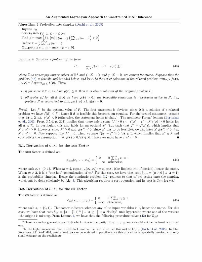
Algorithm 3 Projection onto simplex (Duchi et al., 2008)Input: z0
Sort z0 into y0: y1 ≥ . . . ≥ ymFind ρ = max
{j ∈ [m] | y0j − 1
j
(∑jr=1 y0r − 1
)> 0}
Define τ = 1ρ (∑ρr=1 y0r − 1)
Output: z s.t. zi = max{z0i − τ, 0}.
Lemma 4 Consider a problem of the form
P : minx∈X
f(x) s.t. g(x) ≤ 0, (43)
where X is nonempty convex subset of Rd and f : X→ R and g : X→ R are convex functions. Suppose that theproblem (43) is feasible and bounded below, and let A be the set of solutions of the relaxed problem minx∈X f(x),i.e. A = Argminx∈X f(x). Then:
1. if for some x ∈ A we have g(x) ≤ 0, then x is also a solution of the original problem P ;
2. otherwise (if for all x ∈ A we have g(x) > 0), the inequality constraint is necessarily active in P , i.e.,problem P is equivalent to minx∈X f(x) s.t. g(x) = 0.
Proof: Let f∗ be the optimal value of P . The first statement is obvious: since x is a solution of a relaxedproblem we have f(x) ≤ f∗; hence if x is feasible this becomes an equality. For the second statement, assumethat ∃x ∈ X s.t. g(x) < 0 (otherwise, the statement holds trivially). The nonlinear Farkas’ lemma (Bertsekaset al., 2003, Prop. 3.5.4, p. 204) implies that there exists some λ∗ ≥ 0 s.t. f(x) − f∗ + λ∗g(x) ≥ 0 holds forall x ∈ X. In particular, this also holds for an optimal x∗ (i.e., such that f∗ = f(x∗)), which implies thatλ∗g(x∗) ≥ 0. However, since λ∗ ≥ 0 and g(x∗) ≤ 0 (since x∗ has to be feasible), we also have λ∗g(x∗) ≤ 0, i.e.,λ∗g(x∗) = 0. Now suppose that λ∗ = 0. Then we have f(x)− f∗ ≥ 0, ∀x ∈ X, which implies that x∗ ∈ A andcontradicts the assumption that g(x) > 0,∀x ∈ A. Hence we must have g(x∗) = 0.
B.1. Derivation of quad for the xor Factor
The xor factor is defined as:
φxor(x1, . . . , xm) ={
0 if∑mi=1 xi = 1
−∞ otherwise, (44)
where each xi ∈ {0, 1}. When m = 2, exp(φxor(x1, x2)) = x1 ⊕ x2 (the Boolean xor function), hence the name.When m > 2, it is a “one-hot” generalization of ⊕.3 For this case, we have that conv Sxor = {z ≥ 0 | 1>z = 1}is the probability simplex. Hence the quadratic problem (12) reduces to that of projecting onto the simplex,which can be done efficiently by Alg. 3. This algorithm requires a sort operation and its cost is O(m logm).4
B.2. Derivation of quad for the or Factor
The or factor is defined as:
φor(x1, . . . , xm) ={
0 if∑mi=1 xi ≥ 1
−∞ otherwise, (45)
where each xi ∈ {0, 1}. This factor indicates whether any of its input variables is 1, hence the name. For thiscase, we have that conv Sor = {z ∈ [0, 1]m | 1>z ≥ 1} is a “faulty” unit hypercube where one of the vertices(the origin) is missing. From Lemma 4, we have that the following procedure solves (42) for Sor:
3There is another generalization of ⊕ which returns the parity of x1, . . . , xm; ours should not be confused with thatone.
4In the high-dimensional case, a red-black tree can be used to reduce this cost to O(m) (Duchi et al., 2008). In lateriterations of DD-ADMM, great speed ups can be achieved in practice since this procedure is repeatedly invoked with onlysmall changes on the coefficients.
An Augmented Lagrangian Approach to Constrained MAP Inference
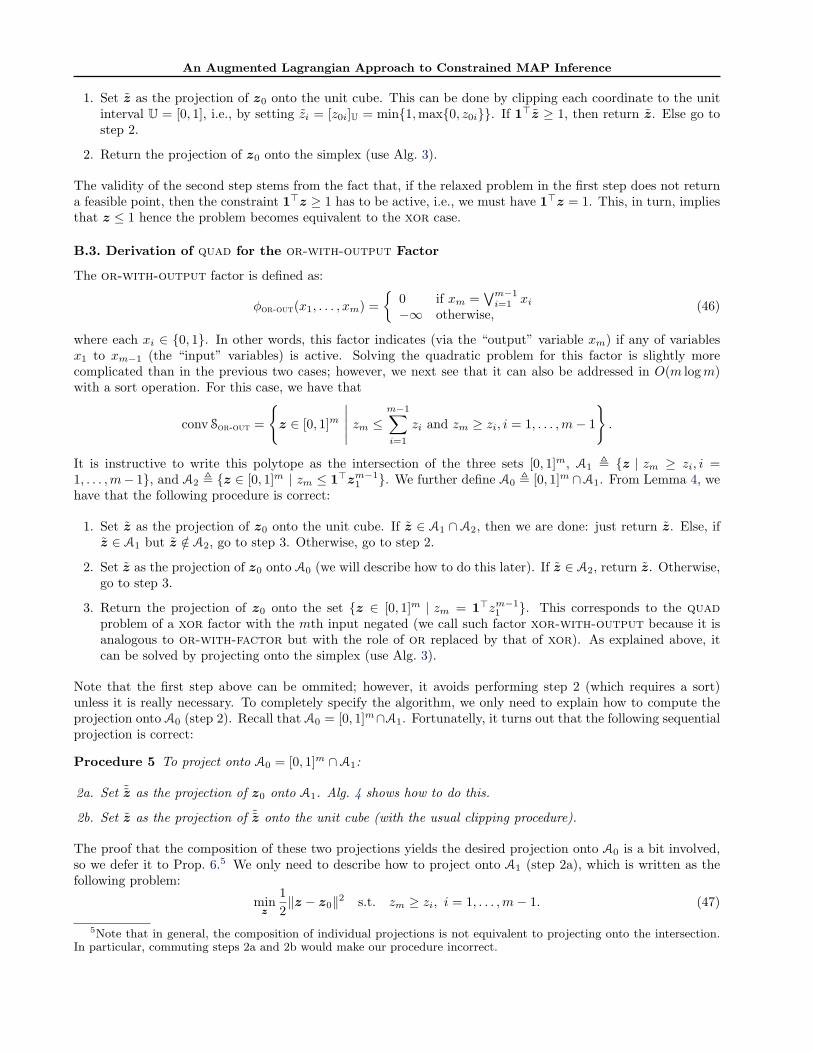
1. Set z as the projection of z0 onto the unit cube. This can be done by clipping each coordinate to the unitinterval U = [0, 1], i.e., by setting zi = [z0i]U = min{1,max{0, z0i}}. If 1>z ≥ 1, then return z. Else go tostep 2.
2. Return the projection of z0 onto the simplex (use Alg. 3).
The validity of the second step stems from the fact that, if the relaxed problem in the first step does not returna feasible point, then the constraint 1>z ≥ 1 has to be active, i.e., we must have 1>z = 1. This, in turn, impliesthat z ≤ 1 hence the problem becomes equivalent to the xor case.
B.3. Derivation of quad for the or-with-output Factor
The or-with-output factor is defined as:
φor-out(x1, . . . , xm) ={
0 if xm =∨m−1i=1 xi
−∞ otherwise,(46)
where each xi ∈ {0, 1}. In other words, this factor indicates (via the “output” variable xm) if any of variablesx1 to xm−1 (the “input” variables) is active. Solving the quadratic problem for this factor is slightly morecomplicated than in the previous two cases; however, we next see that it can also be addressed in O(m logm)with a sort operation. For this case, we have that
conv Sor-out =
{z ∈ [0, 1]m
∣∣∣∣∣ zm ≤m−1∑i=1
zi and zm ≥ zi, i = 1, . . . ,m− 1
}.
It is instructive to write this polytope as the intersection of the three sets [0, 1]m, A1 , {z | zm ≥ zi, i =1, . . . ,m− 1}, and A2 , {z ∈ [0, 1]m | zm ≤ 1>zm−1
1 }. We further define A0 , [0, 1]m ∩A1. From Lemma 4, wehave that the following procedure is correct:
1. Set z as the projection of z0 onto the unit cube. If z ∈ A1 ∩ A2, then we are done: just return z. Else, ifz ∈ A1 but z /∈ A2, go to step 3. Otherwise, go to step 2.
2. Set z as the projection of z0 onto A0 (we will describe how to do this later). If z ∈ A2, return z. Otherwise,go to step 3.
3. Return the projection of z0 onto the set {z ∈ [0, 1]m | zm = 1>zm−11 }. This corresponds to the quad
problem of a xor factor with the mth input negated (we call such factor xor-with-output because it isanalogous to or-with-factor but with the role of or replaced by that of xor). As explained above, itcan be solved by projecting onto the simplex (use Alg. 3).
Note that the first step above can be ommited; however, it avoids performing step 2 (which requires a sort)unless it is really necessary. To completely specify the algorithm, we only need to explain how to compute theprojection onto A0 (step 2). Recall that A0 = [0, 1]m∩A1. Fortunatelly, it turns out that the following sequentialprojection is correct:
Procedure 5 To project onto A0 = [0, 1]m ∩A1:
2a. Set ˜z as the projection of z0 onto A1. Alg. 4 shows how to do this.
2b. Set z as the projection of ˜z onto the unit cube (with the usual clipping procedure).
The proof that the composition of these two projections yields the desired projection onto A0 is a bit involved,so we defer it to Prop. 6.5 We only need to describe how to project onto A1 (step 2a), which is written as thefollowing problem:
minz
12‖z − z0‖2 s.t. zm ≥ zi, i = 1, . . . ,m− 1. (47)
5Note that in general, the composition of individual projections is not equivalent to projecting onto the intersection.In particular, commuting steps 2a and 2b would make our procedure incorrect.
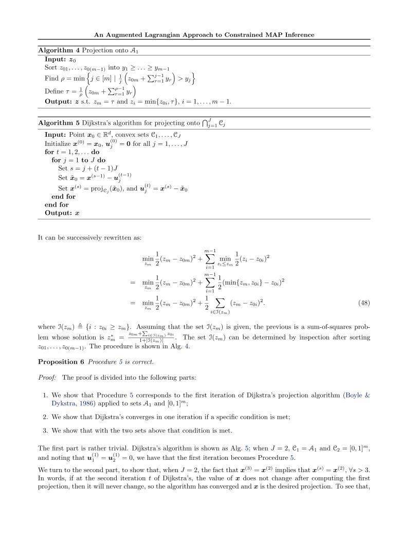
An Augmented Lagrangian Approach to Constrained MAP Inference
Algorithm 4 Projection onto A1
Input: z0
Sort z01, . . . , z0(m−1) into y1 ≥ . . . ≥ ym−1
Find ρ = min{j ∈ [m] | 1
j
(z0m +
∑j−1r=1 yr
)> yj
}Define τ = 1
ρ
(z0m +
∑ρ−1r=1 yr
)Output: z s.t. zm = τ and zi = min{z0i, τ}, i = 1, . . . ,m− 1.
Algorithm 5 Dijkstra’s algorithm for projecting onto⋂Jj=1 Cj
Input: Point x0 ∈ Rd, convex sets C1, . . . ,CJInitialize x(0) = x0, u(0)
j = 0 for all j = 1, . . . , Jfor t = 1, 2, . . . do
for j = 1 to J doSet s = j + (t− 1)JSet x0 = x(s−1) − u(t−1)
j
Set x(s) = projCj(x0), and u(t)
j = x(s) − x0
end forend forOutput: x
It can be successively rewritten as:
minzm
12
(zm − z0m)2 +m−1∑i=1
minzi≤zm
12
(zi − z0i)2
= minzm
12
(zm − z0m)2 +m−1∑i=1
12
(min{zm, z0i} − z0i)2
= minzm
12
(zm − z0m)2 +12
∑i∈I(zm)
(zm − z0i)2. (48)
where I(zm) , {i : z0i ≥ zm}. Assuming that the set I(zm) is given, the previous is a sum-of-squares prob-
lem whose solution is z∗m =z0m+
Pi∈I(zm) z0i
1+|I(zm)| . The set I(zm) can be determined by inspection after sortingz01, . . . , z0(m−1). The procedure is shown in Alg. 4.
Proposition 6 Procedure 5 is correct.
Proof: The proof is divided into the following parts:
1. We show that Procedure 5 corresponds to the first iteration of Dijkstra’s projection algorithm (Boyle &Dykstra, 1986) applied to sets A1 and [0, 1]m;
2. We show that Dijkstra’s converges in one iteration if a specific condition is met;
3. We show that with the two sets above that condition is met.
The first part is rather trivial. Dijkstra’s algorithm is shown as Alg. 5; when J = 2, C1 = A1 and C2 = [0, 1]m,and noting that u(1)
1 = u(1)2 = 0, we have that the first iteration becomes Procedure 5.
We turn to the second part, to show that, when J = 2, the fact that x(3) = x(2) implies that x(s) = x(2), ∀s > 3.In words, if at the second iteration t of Dijkstra’s, the value of x does not change after computing the firstprojection, then it will never change, so the algorithm has converged and x is the desired projection. To see that,
An Augmented Lagrangian Approach to Constrained MAP Inference
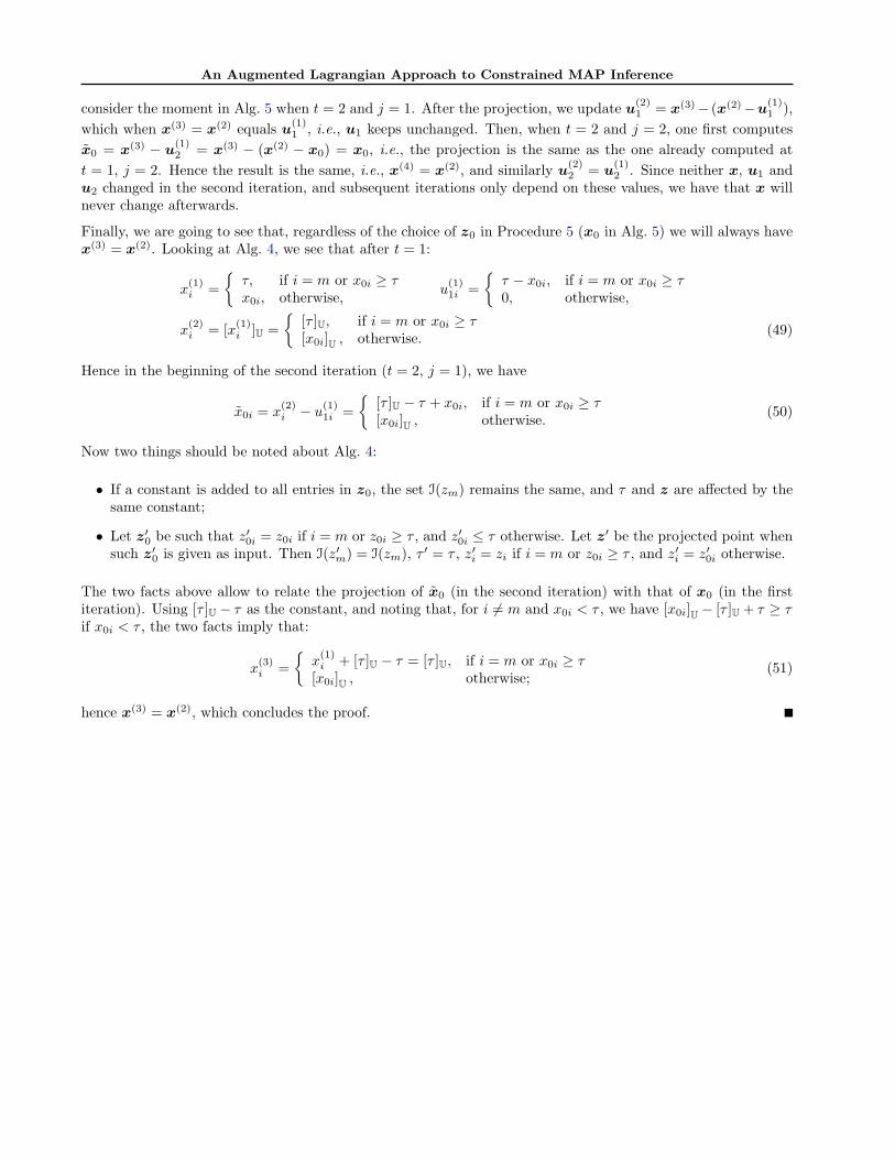
consider the moment in Alg. 5 when t = 2 and j = 1. After the projection, we update u(2)1 = x(3)− (x(2)−u(1)
1 ),which when x(3) = x(2) equals u(1)
1 , i.e., u1 keeps unchanged. Then, when t = 2 and j = 2, one first computesx0 = x(3) − u(1)
2 = x(3) − (x(2) − x0) = x0, i.e., the projection is the same as the one already computed att = 1, j = 2. Hence the result is the same, i.e., x(4) = x(2), and similarly u(2)
2 = u(1)2 . Since neither x, u1 and
u2 changed in the second iteration, and subsequent iterations only depend on these values, we have that x willnever change afterwards.
Finally, we are going to see that, regardless of the choice of z0 in Procedure 5 (x0 in Alg. 5) we will always havex(3) = x(2). Looking at Alg. 4, we see that after t = 1:
x(1)i =
{τ, if i = m or x0i ≥ τx0i, otherwise, u
(1)1i =
{τ − x0i, if i = m or x0i ≥ τ0, otherwise,
x(2)i = [x(1)
i ]U ={
[τ ]U, if i = m or x0i ≥ τ[x0i]U , otherwise. (49)
Hence in the beginning of the second iteration (t = 2, j = 1), we have
x0i = x(2)i − u
(1)1i =
{[τ ]U − τ + x0i, if i = m or x0i ≥ τ[x0i]U , otherwise. (50)
Now two things should be noted about Alg. 4:
• If a constant is added to all entries in z0, the set I(zm) remains the same, and τ and z are affected by thesame constant;
• Let z′0 be such that z′0i = z0i if i = m or z0i ≥ τ , and z′0i ≤ τ otherwise. Let z′ be the projected point whensuch z′0 is given as input. Then I(z′m) = I(zm), τ ′ = τ , z′i = zi if i = m or z0i ≥ τ , and z′i = z′0i otherwise.
The two facts above allow to relate the projection of x0 (in the second iteration) with that of x0 (in the firstiteration). Using [τ ]U − τ as the constant, and noting that, for i 6= m and x0i < τ , we have [x0i]U − [τ ]U + τ ≥ τif x0i < τ , the two facts imply that:
x(3)i =
{x
(1)i + [τ ]U − τ = [τ ]U, if i = m or x0i ≥ τ
[x0i]U , otherwise;(51)
hence x(3) = x(2), which concludes the proof.