Open Journal of Forestry 2012. Vol.2, No.2, 41-53 Published Online April 2012 in SciRes (http://www.SciRP.org/journal/ojf) DOI:10.4236/ojf.2012.22006

An Assessment of Flowering Dogwood (Cornus florida L.) Decline in the Eastern United States

Christopher M. Oswalt1, Sonja N. Oswalt1, Christopher W. Woodall2 1Forest Inventory and Analysis, United States Department of Agriculture Forest

Service Southern Research Station, Knoxville, USA 2Forest Inventory and Analysis, United States Department of Agriculture Forest

Service Northern Research Station, St. Paul, USA Email: soswalt@fs.fed.us

Received February 19th, 2012; revised March 23rd, 2012; accepted March 31st, 2012

Cornus florida L. is one of the most numerous tree species in the Eastern United States (US). Multiple studies have reported localized declines in C. florida populations following the introduction of the de-structive fungus Discula destructiva Redlin (dogwood anthracnose), but few, if any, have documented changes in C. florida populations across the species’ entire natural range. Thus, a current assessment of the C. florida population in the Eastern US and implications for future sustainability is warranted. Our study’s goal was to present C. florida population estimates across the natural range of the species (Little, 1971) in the Eastern US for two periods based on state-level forest land inventories conducted by the US Department of Agriculture Forest Service, Forest Inventory and Analysis (FIA) program. Rangewide, C. florida populations declined by approximately 49% over the time periods studied. At the State level, population declines occurred in 17 out of 30 states and biomass declines occurred in 20 out of 30 states studied. While declines were widespread in the substate units surrounding the Appalachians, the largest declines appeared to be centered within the Appalachian ecoregion. Keywords: Forest Inventory; Population Decline; Tree Disease; Discula destructiva

Introduction

Cornus florida L. (flowering dogwood) is widely distributed across the eastern landscape of the United States (US) and is one of the most common understory trees in North America (Jenkins & White, 2002). Little (1971) describes the C. florida geographical distribution as covering the majority of the East-ern US from northern Florida and the Gulf Coast to southern Michigan and New England and extending as far west as east-ern Oklahoma and eastern Texas. Although C. florida is an important member of the eastern deciduous forest, the species has been and is currently experiencing localized and regional declines. Cornus florida declines have largely been attributed to an imported fungus (Britton, 1994). The fungus Discula de-structiva Redlin (dogwood anthracnose) (Mielke & Langdon, 1986; Redlin, 1991; Chellimi et al., 1992) has been identified as responsible for considerable C. florida mortality throughout the East, particularly in the Appalachian ecoregion (Oswalt & Oswalt, 2010).

Botanical surveys conducted throughout the 20th Century have documented the abundance of C. florida in the Eastern US (Hiers & Evans, 1997). Measures of high relative density and elevated importance values prior to D. destructiva infestation were reported by Hannah (1993) in North Carolina, Quarter-man et al. (1972) in Tennessee, Muller (1982) in Kentucky, Carr and Banas (2000) in Virginia, and Sherald et al. (1996) in Maryland. Moreover, C. florida has been documented as a common component of second-growth hardwood stands (Orwig & Abrams, 1994; Jenkins & Parker, 1998), as an important understory component of old-growth forests (McCune et al.,

1988; Goebel & Hix, 1996), and is also reported to be a sig- nificant source of calcium, in the form of leaf litter, in the sur- face horizons of some forest soils (Thomas, 1969; Hepting, 1971).

Multiple studies (Hiers & Evans, 1997; Schwegman et al., 1998; Williams & Moriarty, 1999; McEwan et al., 2000) have reported substantial C. florida mortality at local scales across its natural biological range following local colonization by D. destructiva, the causal agent for dogwood anthracnose (Redlin, 1991). While numerous studies have quantified local losses of C. florida (Sherald et al., 1996; Hiers & Evans, 1997; Schwegman et al., 1998; Williams & Moriarty, 1999; Carr & Banas, 2000; McEwan et al., 2000) specifically attributed to D. destructiva, few, if any, studies have quantified large-scale losses across the entire range of C. florida. Given that C. flor-ida is one of the most numerous tree species in the Eastern U.S. (Woodall et al., 2010), a current assessment of the C. florida population in the Eastern US and implications for future sus-tainability is warranted. While D. destructiva is a known pathogen that has had documented negative impacts on C. flor- ida populations, the decline of C. florida is ultimately a combi- nation of numerous causal agents, including inter-and intra- specific competition, defoliators, and a lack of management or restoration of the species. Setting aside the complexities of abiotic and biotic decline agents, much can be gained from a strategic-scale assessment of C. florida population changes known to be experiencing localized declines using comparisons of large-scale forest inventories. Hence, our study’s goal was to present C. florida population estimates across the natural range of the species (Little, 1971) in the Eastern US for two periods

Copyright © 2012 SciRes. 41

C. M. OSWALT ET AL.

based on state-level forest land inventories conducted by the US Department of Agriculture (USDA) Forest Service, Forest Inventory and Analysis (FIA) program. Our specific objectives were to: (1) quantify current C. florida populations in the East-ern US, (2) quantify change, if any, in C. florida populations for the period beginning in the early 1980s to 2007 and (3) identify regional and spatial trends in C. florida population shifts for the same period.

Materials and Methods

Data

The forest inventory conducted by FIA is a year-round effort to collect and disseminate information and statistics on the extent, condition, status and trends of forest resources across all ownerships (Smith 2002). In the late 1990s, FIA began a transi-tion from irregular and asynchronous periodic inventories to annual inventories (Bechtold & Patterson, 2005). Before 2000, most inventories were periodic; since 2000 most states have been inventoried annually. FIA applies a nationally consistent sampling protocol using a quasisystematic design covering all ownerships in the entire Nation (Bechtold & Patterson, 2005). For this study, data was collected across 41 FIA regional units among 13 states. Fixed-area plots were installed in locations with accessible forest land cover (Bechtold & Patterson, 2005). Field crews collected data on >300 variables, including land ownership, forest type, tree species, tree size, tree condition, and other site attributes (e.g., slope, aspect, disturbance, land use) (Smith, 2006; US Department of Agriculture, 2004). Plot intensity for field collected data was approximately one plot for every 2400 ha (6000 acres) of land (125,000 plots nation-ally).

The design for FIA inventory plots consists of four 7.3 m fixed-radius subplots spaced 36.6 m apart in a triangular ar-rangement with one subplot in the center (Bechtold & Patterson, 2005). All trees with a diameter at breast height (d.b.h.) of at least 12.7 cm are inventoried on forested subplots. A 2.1 m radius microplot, offset 3.7 m from subplot center, is estab-lished within each subplot. All live tree seedlings are tallied according to species within each microplot. Conifer seedlings must be at least 15.2 cm in length with a root collar diameter < 2.54 cm to qualify for measurement. Hardwood seedlings must be at least 3.5 cm in length with a root collar diameter < 2.54 cm to qualify for measurement.

Data were assembled from the USDA Forest Service, FIA database (FIADB) version 3.0 in May 2009 (US Department of Agriculture, 2006). The FIADB contains both current and his-toric inventory data related to the forest resources of the U.S. (Reams et al., 2005). County level estimates of C. florida populations (number of all live trees > 2.54 cm d.b.h.) and total C. florida biomass (tons of all live trees > 2.54 cm d.b.h.) were generated for all states (except Oklahoma) within the historic range of C. florida (Little, 1971) from FIA plot data for two periods in time and labeled time 1 and time 2 (Table 1). Perfect alignment of inventory dates was not possible due to the nature of past periodic inventories and variability in transition times between periodic and annual inventory designs (Bechtold & Patterson, 2005). Similarly, county-level population estimates were necessary because of the lack of complete plot alignment due to an altered plot design (variable radius to fixed radius) between periodic and annual inventory implementation. The

data labeled time 1 ranged from 1983 in Nebraska to 1995 in Arkansas and Maine (Table 1) roughly corresponds to the time around which D. destructiva was first identified as a causal agent for dogwood anthracnose (Mielke & Langdon, 1986; Redlin, 1991; Chellemi et al., 1992), and represents a time pe-riod early in the spread of the disease. The data labeled time 2 was less variable and ranged from 2005 to 2007. Individual counties were assigned to FIA substate units that correspond to both political and ecological boundaries (Figure 1).

Table 1. State and inventory data selected for analysis by time period grouping.

Time 1 Time 2 State

periodic annual

Alabama 1990 2007

Arkansas 1995 2007

Connecticut 1985 2006

Delaware 1986 2006

Florida 1987 2007

Georgia 1989 2007

Illinois 1985 2007

Indiana 1986 2007

Iowa 1990 2007

Kansas 1994 2007

Kentucky 1988 2006

Louisiana 1991 2005

Maine 1995 2006

Maryland 1986 2006

Massachusetts 1985 2006

Michigan 1993 2007

Minnesota 1990 2007

Mississippi 1994 2006

Missouri 1989 2007

Nebraska 1983 2007

New Jersey 1987 2006

New York 1993 2006

North Carolina 1984 2006

Ohio 1991 2006

Pennsylvania 1989 2006

Rhode Island 1985 2006

South Carolina 1986 2007

Tennessee 1989 2007

Texas 1992 2007

Virginia 1984 2007

West Virginia 1989 2006

Copyright © 2012 SciRes. 42

C. M. OSWALT ET AL.

Copyright © 2012 SciRes. 43

Figure 1. Historic range of Cornus florida (L.) shown with state boundaries and Forest Inventory and Analysis (FIA) units (see Table A5 for unit code descrip-tions). Analysis

Absolute change, percent change and annual change was cal- culated for each county. Annual change was calculated by di-viding the difference between times 1 and 2 for each county by the remeasurement period. Paired t-tests pairing county-level estimates at times 1 and 2 using R (R Development Core Team, 2009) were used to identify significant changes in C. florida tree populations and total biomass rangewide and within states and regional (FIA) units between times 1 and 2. Additional paired t-tests were used to test for significant changes in tree populations and total biomass within 5.1 cm diameter classes rangewide. Biomass estimates were converted to metric equiva- lents post-analysis.

Results

Rangewide

No C. florida stems were sampled in the states of Vermont, New Hampshire or Wisconsin for the two periods represented in this study. The rangewide C. florida population in the East-ern US declined approximately 49% (P < .0001) from an esti-mated 9.3 billion trees at time 1 to an estimated 4.7 billion trees at time 2 (Table A1). Mean annual change among all states

within the historic range of C. florida equates to losses of ap-proximately 8.6 million trees·year–1 over the period of this study. Total biomass (Mg) declined approximately 58% (P < .0001) from 10.0 million Mg to 41.8 million Mg from time 1 to time 2, respectively (Table A1). Mean annual change was approximately –112,418 Mg·year–1 among all states. All C. florida stems sampled in times 1 and 2 were in the 35.6 cm diameter class or smaller (Table A2). Significant declines in the total number of C. florida stems occurred between time periods for the 5.1, 1.2, 15.2, and 2.3 cm (2, 4, 6 and 8 in.) di-ameter classes (P < .0001, < .0001, < .0001, < .0001, respec-tively), while significant declines in biomass were identified in the 5.1, 1.2, 15.2, 2.3, and 25.4 cm (2, 4, 6, 8, and 10 in.) di-ameter classes (P < .0001, < .0001, < .0001, < .0001, = .0075, respectively). The relative declines in biomass were slightly larger than declines in the number of stems for each of the 5.1 cm (2 in.) diameter classes (Table A3). What appeared to be large relative increases in the 35.6 cm (14 in.) diameter class were not significant for either number of stems or dry biomass (P = .1507 and = .2489, respectively).

State Level

Seventeen out of 30 eastern states experienced significant declines in C. florida populations, while 20 states experienced

C. M. OSWALT ET AL.

significant declines in dry biomass (Table A4). The largest absolute declines in numbers of stems, calculated as mean county change, occurred in Alabama, followed by West Vir-ginia, Virginia, North Carolina and Tennessee with losses of 8.1, 7.5, 6.0, 5.8 and 5.0 million trees, respectively (all p values < .0001). Cornus florida biomass declines were also largest in Alabama (Table A4). Maryland (P = .0038) was the only state where a significant increase in biomass was observed. No sig-nificant increases in numbers of trees were observed. Cornus florida was sampled only for time 1 in Kansas, Maine and Ne-braska and, therefore, relative losses appeared to be 100% (Ta-ble A1), although not significant (Table A4). The largest rela-tive declines in numbers of trees from time 1 to time 2 were observed in West Virginia (–73%; P < .0001), Ohio (–71%; P < .0001), Maryland (–66%; P = .0043) and Pennsylvania (–64%; P < .0001) (Table A1). The largest significant relative declines in biomass occurred in New York (–71%; P = .0194), Ohio (–70%; P < .0001), Mississippi (–69%; P < .0001), Virginia (–68%; P < .0001) and North Carolina (–67%; P < .0001) (Ta-ble A1).

Substate Level

Cornus florida stems were recorded in 107 FIA units in ei-ther times 1 or 2 or at both times (Table A5). Significant de-clines in numbers of stems were observed in 57 units (53%). Dry biomass declined in 55 (51%) of the 105 FIA units. Sig-nificant declines in both numbers of stems and dry biomass were detected in 48 units (45%). The largest regional declines in number of stems were in southwest-north Alabama (–16.4 million trees·county–1, P = .0035) and southern West Virginia (–13.9 million trees·county–1, P < .0001). Biomass loss was greatest in southwest-north Alabama (–244,723 Mg·county–1, P = .0105) and west central Alabama (–188,035 Mg·county–1, P < .0023). Losses, both in terms of number of stems and biomass, appeared to be heaviest within the Appalachian Mountains and surrounding area. Interestingly, significant regional increases in number of stems (P = .0280) and biomass (P = .0294) were observed in the South Delta unit in Louisiana which is outside of the geographic distribution delineated by Little (1971).

The largest substate declines relative to the time 1 population occurred in New York. The Adirondack and South-central Highlands units experienced a 100% loss of C. florida stems (P = .0419 and = .0233, respectively). Sixteen percent of all sub-state units experienced calculated declines of >75%. Calculated relative declines in excess of 50% were recorded in 53% of all FIA units. Relative increases in stem numbers, regardless of statistical significance, were observed in 16% of units. Signifi-cant increases in numbers of stems were observed in the Southwestern Ozarks of Missouri (P = .0193) and in the South Delta of Louisiana (P = .0280).

Discussion

The results of this investigation suggest that C. florida popu-lations have declined significantly across the Eastern US De-clines in absolute numbers of trees have been particularly no-ticeable in the Appalachians and in the South. Losses relative to population levels during the period of 1983-1995 (time 1) ap-peared larger in the North. One reason for this may be that the majority of the data for time 1 was collected in the late 1980s and early 1990s. Symptoms of what was once labeled “lower

branch dieback” (Daughtrey & Hibben, 1983) but eventually described as D. destructiva (Redlin, 1991) were first recognized in New York in the spring of 1979 (Daughtrey et al., 1996). Therefore, many stems could have succumbed to D. destructiva and not have been sampled in the northern FIA inventories during the late 1980s. However, the southern FIA inventories may not have been impacted due to the lag time that would result from the movement of D. destructiva migration south-ward.

This analysis does not discriminate among causal agents of C. florida mortality. However, with declines correlating geo-graphically with the known D. destructiva distribution coupled with numerous localized investigations implicating D. destruc-tiva in significant C. florida losses, it can be assumed that D. destructiva has had a significant impact on populations in the region. While the assumption of the authors is that a significant amount of the C. florida declines revealed by this investigation can be attributed to the impacts of the fungus D. destructiva, other factors are likely to have played some role, particularly in states where D. destructiva has not been identified as problem-atic (e.g., Mississippi). For example, Pierce (2001), in Indiana, attributed C. florida mortality to competition with Acer sac-charum and mediated by fire suppression activities. In Ken-tucky, McEwan et al. (2000) reported a 36% decline in C. flor-ida density in an old-growth stand prior to the documentation of D. destructiva in the area. While it is possible D. destructiva was present without having been documented, McEwan et al. (2000) suggested that factors such as canopy closure, drought, and natural canopy-gap dynamics may have been an important factor. That theory is supported by a study by Oswalt and Oswalt (2010), which found that changes in C. florida popula-tions were significantly related to changes in all live volumes of forest density. The well documented deleterious impacts of D. destructiva, however, cannot be ignored. According to reports from Anderson (1991) and Knighten and Anderson (1992, 1993), D. destructive-mediated C. florida mortality increased from 0% to 23% in the Appalachians between 1988 and 1993. Concomitantly, the area estimated to be infected with D. de-structiva increased from 0.2 to 7.0 million ha over the same period (Daughtrey et al., 1996). Moreover, Windham et al. (1993) reported widespread infection and rapid die-off of C. florida throughout the Great Smoky Mountains National Park in the early 1990s.

While the declines in C. florida populations were significant for this study, loss estimates were generally lower than many of the documented studies at much smaller scales. For example, while the results of this study suggested losses of approxi-mately 60% of the C. florida population in east Tennessee and 74% on the Cumberland Plateau, Hiers and Evans (1997) re-ported C. florida declines of approximately 98% from C. flor-ida population estimates first reported by McGee (1986) in Tennessee. Myers et al. (2004) observed significant declines of C. florida, also on the Cumberland Plateau, and documented the species’ complete disappearance from the subcanopy on their study site. The current study suggests that while the loss amounted to approximately 74% of the C. florida population, declines averaged >10 million stems per county on the Cum-berland Plateau between times 1 and time 2 (Table 1). The loss of C. florida on the Cumberland Plateau in Tennessee during the period of this study was approximately 170 million trees.

In Maryland, C. florida declines averaged between 56 and 79% among four regions between times 1 and 2. Sherald et al.

Copyright © 2012 SciRes. 44

C. M. OSWALT ET AL.

(1996) documented C. florida mortality at approximately 77% between 1976 and 1992. Regional relative declines of C. florida populations in Pennsylvania ranged from 63% to 82% with no change in mean county-level populations estimates in the North Central Allegheny region. Williams and Moriarty (1999) re-ported C. florida mortality in the northern Allegheny Plateau of between 58% and 68%. The lack of significant change in some parts of the Allegheny region could be a result of the lower densities of C. florida documented in the area (Williams & Moriarty, 1999). In some areas, the lack of significant change was possibly due to a limited number of counties in some re-gional FIA units (e.g., Western unit in Maryland has two coun-ties).

It is important to note that the estimates reported here for the period 1983 to 1995 (time 1) were generated during a time when FIA implemented periodic inventories. The estimates generated for the period 2005-07 (time 2) were generated from the FIA program’s annual inventory design (Bechtold & Pat-terson, 2005). As a result, additional uncertainty is introduced when comparing estimates across time. However, analyses at broad scales, such as the one here, reduce the probability of the additional uncertainty significantly influencing the results. Fei and Steiner (2007) used similar methods (time 1 data was from periodic inventories and ranged from 1980-1995 while time 2 data was from annual inventories with a much smaller range) to identify large-scale increases in Acer rubrum populations in eastern forests. Regional differences as a result of FIA organ-izational structure between the North and South are recognized during implementation of both the periodic and annual invento-ries. However, focus on tree level variables minimizes the im-pact of such differences.

Given the documented range of dogwood prior to 1971 (Lit-tle, 1971) and its substantial decline from the 1980s to the pre-sent, we hypothesize that future dogwood populations will con-tinue to wane. The deleterious effects of D. destructiva, com-bined with inter- and intra-specific competition, defoliators, and little emphasis on restoration and management engenders little hope for slowing the decline of C. florida populations on the landscape. Additionally, climate change effects might be ex-pected to negatively affect C. florida populations. The rela-tively widespread C. florida range could ensure its stability in limited southern locations, while the majority of its extent in the middle and high latitudes may face increased competition due to climate-change induced species migration (Woodall et al., 2009). Some evidence from this study suggests that range shifts may already be occurring in C. florida populations given that the greatest losses in biomass occurred in the species’ northern range and greatest gains occurred in its southern range. However, range shifts were not the focus of this study and fur-ther investigation and monitoring over time will be necessary to corroborate those initial observations. Although the future range and magnitude of C. florida populations is uncertain, the need for continued monitoring and proactive approaches to restoration and management is evident.

Conclusion

While declines were widespread in the substate units sur-rounding the Appalachians, the largest declines appeared to be centered within the Appalachian ecoregion. These results indi-cate that an important component of the eastern deciduous for-est may be suffering serious declines. Our results support many

smaller, localized investigations of C. florida mortality as well as large quantities of anecdotal evidence that has been accumu-lated over time. Cornus florida has been an important tree spe-cies in the Appalachian ecoregion. Faced with large-scale de-clines in populations of C. florida, particularly in the midstory of eastern deciduous forests, further expansion of generalist species such as A. rubrum may be expected to occur. The need for continued monitoring and proactive restoration and man-agement goals for C. florida is evident.

Acknowledgements

The authors thank the USDA Forest Service Southern Re-search Station (SRS) and Northern Research Station (NRS) for funding and support for this project. We also acknowledge the hard work and dedication of SRS and NRS field crews.

REFERENCES

Anderson, R. L. (1991). Results of the 1990 dogwood anthracnose impact assessment and pilot test in the southeastern United States. Protection Report R8-PR 20. Atlanta, GA: US Department of Agri-culture Forest Service, Southern Region.

Bechtold, W. A., & Patterson, P. L. (2005). The enhanced forest inven-tory and analysis program—National sampling design and estima-tion procedures. General Technical Report SRS-80. Asheville, NC: US Department of Agriculture Forest Service, Southern Research Station.

Britton, K. O. (1994). Dogwood anthracnose. In C. Ferguson, & P. Bowman (Eds.), Threats to forest health in the southern Appalachi-ans (pp. 17-20). Gatlinburg, TN: Southern Appalachian Man and the Biosphere Co-operative.

Carr, D. E., & Banas, L. E. (2000). Dogwood anthracnose (discula destructiva): Effects of and consequences for host (Cornus florida) demography. American Midland Naturalist, 143, 169-177. doi:10.1674/0003-0031(2000)143[0169:DADDEO]2.0.CO;2

Chellemi, D. O., Britton, K. O., & Swank, W. T. (1992). Influence of site factors in dogwood anthracnose in the Nantahala Mountain range of western North Carolina. Plant Disease, 76, 915-918. doi:10.1094/PD-76-0915

Daughtrey, M. L., & Hibben, C. R. (1983). Lower branch dieback, a new disease of northern dogwoods. Phytopathology, 73, 365.

Daughtrey, M. L., Hibben, C. R., Britten, K. O., Windham, M. T., & Redlin, S. C. (1996). Dogwood anthracnose, understanding a disease new to North America. Plant Disease, 80, 349-358. doi:10.1094/PD-80-0349

Fei, S., & Steiner, K. C. (2007). Evidence for increasing red maple abundance in the eastern United States. Forest Science, 53, 473-477.

Goebel, P. C., & Hix, D. M. (1996). Development of mixed-oak forests in southeastern Ohio: a comparison of second-growth and old-growth forests. Forest Ecology and Management, 84, 1-21. doi:10.1016/0378-1127(96)03772-3

Hannah, P. R. (1993). Composition and development of two Appala-chian hardwood stands in North Carolina. Journal of the Elisha Mitchell Scientific Society, 109, 87-98.

Hepting, G. H. (1971). Diseases of forest and shade trees of the United States. Agriculture Handbook, US Department of Agriculture, Wash-ington DC.

Hiers, J. K., & Evans, J. P. (1997). Effects of anthracnose on dogwood mortality and forest composition of the Cumberland Plateau (USA). Conservation Biology, 11, 1430-1435. doi:10.1046/j.1523-1739.1997.97009.x

Holzmueller, E., Jose, S., Jenkins, M., Camp, A., & Long, A. (2006). Dogwood anthracnose in eastern hardwood forests: What is known and what can be done? Journal of Forest, 104, 21-26.

Jenkins, M. A., & Parker, G. R. (1998). Composition and diversity of woody vegetation in silvicultural openings of southern Indiana for-ests. Forest Ecology and Management, 109, 57-74.

Copyright © 2012 SciRes. 45

C. M. OSWALT ET AL.

Copyright © 2012 SciRes. 46

doi:10.1016/S0378-1127(98)00256-4 Jenkins, M. A., & White, P. S. (2002). Cornus florida L. mortality and

understory composition changes in western Great Smoky Mountains National Park. Journal of the Torrey Botanical Society, 129, 194- 206. doi:10.2307/3088770

Knighten, J. L., & Anderson, R. L. (1992). Results of the 1991 dog-wood anthracnose impact assessment and pilot test in the southeast-ern United States. Protection Report R8-PR 23, US Department of Agriculture Forest Service, Southern Region.

Knighten, J. L., & Anderson, R. L. (1993). Results of the 1992 dog-wood anthracnose impact assessment and pilot test in the southeast-ern United States. Protection Report R8-PR 24, US Department of Agriculture Forest Service, Southern Region.

Little, E. L. Jr. (1971). Atlas of United States trees, volume 1, conifers and important hardwoods. US Department of Agriculture Miscella-neous Publication 1146.

McCune, B., Cloonan, C. L., & Armentano, T. V. (1988). Tree mortal-ity and vegetation dynamics in Hemmer Woods, Indiana. American Midland Naturalist, 120, 416-431. doi:10.2307/2426014

McEwan, R. W., Muller, R. N., Arthur, M. A., & Housman, H. H. (2000). Temporal and ecological patterns of flowering dogwood mortality in the mixed mesophytic forests of eastern Kentucky. Journal of the Torrey Botanical Society, 127, 221-229. doi:10.2307/3088759

McGee, C. E. (1986). Loss of Quercus spp. dominance in an undis-turbed old-growth forest. Journal of the Elisha Mitchell Scientific Society, 102, 10-15.

Mielke, M. and Langdon, K. (1986). Dogwood anthracnose fungus threatens Catoctin Mountain Park. Park Science, 6, 6-8.

Muller, R. N. (1982). Vegetation patterns in the mixed mesophytic forest of eastern Kentucky. Ecology, 63, 1901-1917. doi:10.2307/1940129

Myers, B. R., Walck, J. L., & Blum, K. E. (2004). Vegetation change in a former chestnut stand on the Cumberland Plateau of Tennessee during and 80-year period (1921-2000). Castanea, 69, 81-91. doi:10.2179/0008-7475(2004)069<0081:VCIAFC>2.0.CO;2

Omernik, J. M. (1987). Ecoregions of the conterminous United States. Map (scale 1:7,500,000). Annals of the Association of American Ge-ographers, 77, 118-125.

Orwig, D. A., & Abrams, M. D. (1994). Land-use history (1720-1992), composition, and dynamics of oak-pine forests within the Piedmont and Coastal Plain of northern Virginia. Canadian Journal of Forest Research, 24, 1216-1225. doi:10.1139/x94-160

Oswalt, C. M., & Oswalt, S. N. (2010). Documentation of significant losses in Cornus florida L. populations throughout the Appalachian ecoregion. International Journal of Forestry Research, 2010. doi:10.1155/2010/401951.

Pierce, A. A. (2001). Population dynamics of flowering dogwood (Cor-nus florida L.) and community structure at the Ross biological re-serve. M.S. Thesis, West Lafayette, IN: Purdue University.

Quarterman, E., Turner, B. H., & Hemmerly, T. E. (1972). Analysis of virgin mixed mesophytic forests in Savage Gulf, Tennessee. Bulletin of the Torrey Botanical Club, 99, 228-232. doi:10.2307/2484607

R Development Core Team (2009). R: A language and environment for

statistical computing. R Foundation for Statistical Computing, Vi-enna. http://www.R-project.org

Reams, G. A., Smith, W. D., Hansen, M. H., Bechtold, W. A., Roesch, F. A., & Moisen, G. G. (2005). The forest inventory and analysis sampling frame. General Technical Report SRS-80, Asheville, NC: US Department of Agriculture Forest Service, Southern Research Station.

Redlin, S. C. (1991). Discula destructiva sp. nov., cause of dogwood anthracnose. Mycologia, 83, 633-642. doi:10.2307/3760218

Schwegman, J. E., McClain, W. E., Esker, T. L., & Ebinger, J. E. (1998). Antracnose-caused mortality of flowering dogwood (Cornus florida L.) at Dean Hills Nature Preserve, Fayette County, Illinois, USA. Natural Areas Journal, 18, 204-207.

Sherald, J. L., Stidham, T. M., Hadidian, J. M., & Hoeldtke, J. E. (1996). Progression of the dogwood anthracnose epidemic and the status of flowering dogwood in Catoctin Mountain Park. Plant Dis-ease, 80, 310-312. doi:10.1094/PD-80-0310

Smith, W. B. (2002). Forest inventory and analysis: A national inven-tory and monitoring program. Environmental Pollution, 116, 233- 242. doi:10.1016/S0269-7491(01)00255-X

Smith, W. B. (2006). An overview of inventory and monitoring and the role of FIA in national assessments. Proceedings RMRS-P=42CD. Fort Collins, CO: US Department of Agriculture Forest Service, Rocky Mountain Research Station.

Thomas, W. A. (1969). Accumulation and cycling of calcium by dog-wood trees. Ecological Monographs, 39, 101-120. doi:10.2307/1950739

US Department of Agriculture (2004). Field instructions for southern forest inventory. Unpublished report. Knoxville, TN: Southern Re-search Station, Forest Inventory and Analysis.

US Department of Agriculture (2006). FIA field methods for phase 3 measurements. Version 3.0. Arlington, VA: US Department of Agri-culture Forest Service, Forest Inventory and Analysis Program. http://fia.fs.fed.us/library/field-guides-methods-proc

Williams, C. E., & Moriarity, W. J. (1999). Occurrence of flowering dogwood (Cornus florida L.) mortality by dogwood anthracnose (Discula destructiva Redlin), on the northern Allegheny Plateau. Journal of the Torrey Botanical Society, 126, 313-319. doi:10.2307/2997315

Windham, M. T., Montgomery-Dee, M. E., & Parham, J. (1993). Site parameters that affect dogwood anthracnose incidence and severity. In B. L. James (Ed.), Proceedings of the 38th Southern Nursery Re-search Conference (pp. 184-187). Marietta, GA: Southern Nursery-men’s Association.

Woodall, C. W., Oswalt, C. M., Westfall, J. A., Perry, C. H., & Nelson, M. D. (2009). Tree migration detection through comparisons of his-toric and current forest inventories. Proceedings RMRS-P-56CD. Fort Collins, CO: US Department of Agriculture Forest Service, Rocky Mountain Research Station.

Woodall, C. W., Oswalt, C. M., Westfall, J. A., Perry, C. H., Nelson, M. D., & Finley, A. O. (2010). Selecting tree species for testing climate change migration hypotheses using forest inventory data. Forest Ecology and Management, 259, 778-785. doi:10.1016/j.foreco.2009.07.022

C. M. OSWALT ET AL.

Appendix

Table A1. Estimates of the number of trees (a) and aboveground biomass (b) of dogwood for times 1 and 2 along with sampling error, annualized and relative change for each state.

(a)

Time 1 Time 2 State

Trees Sampling error n plots Trees Sampling error n plots

Annualized change

Relative change (%)

Alabama 1,092,781,586 50,158,675 4515 551,279,079 26,847,291 5375 –31,853,089 –49.6

Arkansas 695,217,351 32,258,085 5878 412,492,486 21,490,859 5571 –23,560,405 –40.7

Connecticut 2,666,645 1,998,917 344 6,018,066 2,708,130 352 159,591 125.7

Delaware 9,936,015 6,829,023 200 3,399,814 1,726,086 244 –326,810 –65.8

Florida 54,537,078 7,182,533 12,441 42,081,521 8,832,911 6,781 –622,778 –22.8

Georgia 810,863,469 27,812,617 12,015 469,478,198 25,680,457 6252 –18,965,848 –42.1

Illinois 65,072,594 6,299,027 10,956 72,839,330 10,467,012 6028 353,033 11.9

Indiana 194,670,206 9,188,434 11,439 95,374,628 8,936,603 4644 –4,728,361 –51

Iowa 421,023 271,728 12,767 347,740 400,944 6018 –4,311 –17.4

Kansas 239,876 299,221 14,875 - - - –18,452 –

Kentucky 622,999,161 43,859,141 3239 343,061,256 19,828,941 4280 –15,552,106 –44.9

Louisiana 192,997,713 18,508,481 2893 125,069,753 12,982,240 5449 –4,851,997 –35.2

Maine 372,484 385,484 3001 - - - –33,862 –

Maryland 71,647,439 15,110,445 1224 24,698,245 6,362,268 548 –2,347,460 –65.5

Massachusetts - - - 1,224,278 1,256,109 566 58,299 –

Michigan 33,119,687 5,203,103 18,483 25,303,000 4,511,525 13,196 –558,335 –23.6

Minnesota - - - 282,382 255,895 17,855 16,611 –

Mississippi 600,732,681 30,276,927 5300 283,426,132 18,280,986 5176 –26,442,212 –52.8

Missouri 529,244,953 15,930,273 17,259 576,198,500 23,393,659 7924 2,608,530 8.9

Nebraska 2,288,061 1,513,095 14,449 - - - –95,336 –

New Jersey 19,876,558 8,946,439 644 10,667,028 6,266,879 417 –484,712 –46.3

New York 31,115,655 6,388,044 5367 11,535,384 4,238,100 3832 –1,506,175 –62.9

North Carolina 931,343,766 28,871,657 9373 359,643,076 22,981,193 4565 –25,986,395 –61.4

Ohio 416,455,023 24,904,010 5056 120,156,133 12,400,113 4356 –19,753,259 –71.1

Pennsylvania 199,013,009 17,891,270 5447 71,699,850 13,056,543 4676 –7,489,009 –64

Rhode Island 3,233,847 3,027,204 100 1,289,850 736,246 140 –92,571 –60.1

South Carolina 340,599,514 16,519,076 7020 218,043,116 16,505,864 3416 –5,836,019 –36

Tennessee 764,366,052 37,836,120 2950 315,639,335 17,675,803 4449 –24,929,262 –58.7

Texas 158,475,178 13,644,713 3705 85,545,756 8,734,222 3741 –4,861,961 –46

Virginia 912,976,646 28,393,574 7314 332,856,088 18,273,799 4585 –25,222,633 –63.5

West Virginia 522,150,905 32,112,281 3341 140,680,993 15,488,977 1376 –22,439,407 –73.1

Copyright © 2012 SciRes. 47

C. M. OSWALT ET AL.

(b)

Time 1 Time 2 State

Mg Sampling error n plots Mg Sampling error n plots

Annualized change

Relative change (%)

Alabama 14,681,920 45,285 4515 5,690,852 259,079 5375 –528,886 –61.2

Arkansas 7,175,656 70,683 5878 3,092,813 160,235 5571 –340,237 –56.9

Connecticut 113,247 813 344 93,488 42,608 352 –941 –17.4

Delaware 33,165 687 200 86,072 30,550 244 2645 159.5

Florida 676,545 35,599 12,441 365,771 61,211 6781 –15,539 –45.9

Georgia 9,585,290 128,559 12,015 4,785,739 231,602 6252 –266,642 –50.1

Illinois 509,127 5,466 10,956 300,419 34,315 6028 –9487 –41

Indiana 1,589,255 17,684 11,439 551,966 52,741 4644 –49,395 –65.3

Iowa 1,260 839 12,767 309 357 6018 –56 –75.4

Kansas 525 27,130 14,875 - - - –40 -

Kentucky 6,296,147 93,049 3239 3,615,705 217,727 4280 –148,913 –42.6

Louisiana 2,742,943 91,882 2893 1,534,816 149,570 5449 –86,295 –44

Maine 811 259,955 3001 - - - –74 -

Maryland 69,528 133,572 1224 293,671 65,502 548 11,207 322.4

Massachusetts - - - 12,416 9,022 566 591 -

Michigan 252,253 7,145 18,483 91,411 16,089 13,196 –11,489 –63.8

Minnesota - - - 616 558 17,855 36 -

Mississippi 9,293,321 263,639 5300 2,851,748 174,260 5176 –536,798 –69.3

Missouri 4,151,419 50,126 17,259 2,499,988 110,693 7924 –91,746 –39.8

Nebraska 8,027 106,323 14,449 - - - –334 -

New Jersey 322,914 0 644 227,303 127,288 417 –5032 –29.6

New York 442,769 623,789 5367 130,228 44,569 3832 –24,042 –70.6

North Carolina 10,298,401 489,489 9373 3,446,261 202,293 4565 –311,461 –66.5

Ohio 4,003,046 252,498 5056 1,188,839 115,158 4356 –187,614 –70.3

Pennsylvania 1,481,278 437,786 5447 719,055 99,045 4676 –44,837 –51.5

Rhode Island 12,960 318,677 100 18,859 9,338 140 281 45.5

South Carolina 3,920,441 173,465 7020 2,098,895 140,715 3416 –86,740 –46.5

Tennessee 9,592,100 485,761 2950 3,429,733 196,362 4449 –342,354 –64.2

Texas 1,904,753 182,551 3705 704,505 73,524 3741 –80,017 –63

Virginia 7,147,407 261,572 7314 2,288,775 143,201 4585 –211,245 –68

West Virginia 3,687,075 352,415 3341 1,655,703 186,155 1376 –119,492 –55.1

Copyright © 2012 SciRes. 48

C. M. OSWALT ET AL.

Table A2. Mean difference between times 1 and 2, sample size, t statistic and associated p-value for number of trees and biomass by diameter class for dogwood in the Eastern United States.

Trees (no.) Biomass (Mg) Diameter class n

Mean of difference t2 P3 Mean of difference t2 P3

2 1390 –2,720,635 –21.92 <.0001 –17,018 –23.04 <.0001

4 1390 –503,314 –15.34 <.0001 –19,137 –17.78 <.0001

6 1390 –64,865 –11.76 <.0001 –4759 –13.94 <.0001

8 1390 –4,932 –4.23 <.0001 –865 –6.34 <.0001

10 1390 –600 –1.83 .0682 –171 –2.68 .0075

12 1390 –85 –.86 .3914 –46 –1.46 .1452

14 1390 68 1.44 .1507 30 1.15 .2489

All stems 1390 –3,294,313 –22.76 <.0001 –41,884 –23.08 <.0001

1County-level mean difference of the number of dogwood stems > 2.5 cm (1-inch) diameter between times 1 and 2; 2Paired T-test pairing time 1 county-level estimates to time 2 county-level estimates; 3P-value of paired t-test. Bold numerals denotes significance at the .05 level.

Table A3. Estimates of the number of trees and aboveground biomass of dogwood for times 1 and 2 along with associated sampling error, t statistic, p-value and percent change by diameter class.

Time 1 Sampling error Time 2 Sampling errorDiameter class

Trees (millions) t1 P2 Percent change

2 7,548.80 103.12 3,767.08 67.15 –21.92 <.0001 –50

4 1,486.86 34.8 787.31 22.93 –15.34 <.0001 –47

6 216.54 6.61 126.38 2.97 –11.76 <.0001 –42

8 23.92 1.49 17.06 .91 –4.23 <.0001 –29

10 2.91 .39 2.07 .28 –1.83 .0682 –29

12 .37 .11 .25 .1 –.86 .3914 –32

14+ .02 .02 .11 .06 1.44 .1507 592

Biomass (Mg)

2 39,594,515 607,329 15,939,283 324,914 –23.05 <.0001 –60

4 44,387,753 1,105,408 17,788,644 573,147 –17.78 <.0001 –60

6 12,512,048 396,567 5,897,061 149,144 –13.94 <.0001 –53

8 2,788,154 180,239 1,585,685 89,260 –6.34 <.0001 –43

10 576,669 81,240 338,093 48,256 –2.68 .0075 –41

12 123,230 38,511 58,671 22,941 –1.46 .1452 –52

14+ 11,213 11,370 168,520 89,332 1.15 .2489 1403

1Paired T-test pairing time 1 county-level estimates to time 2 county-level estimates; 2P-value of paired t-test. Bold numerals denotes significance at the .05 level.

Copyright © 2012 SciRes. 49

C. M. OSWALT ET AL.

Table A4. Mean difference between times 1 and 2, sample size, t statistic and associated p-value for number of trees and biomass by state for dogwood in the Eastern United States.

Trees (no.) Biomass (Mg) State n

Mean of difference1 t2 P3 Mean of difference1 t2 P3

Alabama 67 –8,081,781 –7.69 <.0001 –134,192 –8.31 <.0001

Arkansas 72 –3,927,404 –5.39 <.0001 –56,716 –6.19 <.0001

Connecticut 8 418,917 .84 .4313 –2471 –.36 .7328

Delaware 3 –2,181,978 –2.36 .1422 17,634 1.47 .2795

Florida 30 –414,954 –0.87 .3917 –10,359 –1.72 .0958

Georgia 133 –2,567,326 –8.06 <.0001 –36,091 –8.87 <.0001

Illinois 53 146,623 .72 .4747 –3937 –2.99 .0043

Indiana 68 –1,460,115 –4.42 <.0001 –15,253 –5.18 <.0001

Iowa 2 –36,359 –.09 .94 –474 –.61 .6534

Kansas 3 –79,972 –2.77 .1091 –175 –2.35 .143

Kentucky 105 –2,665,048 –6.05 <.0001 –25,513 –4.7 <.0001

Louisiana 44 –1,543,978 –2.46 .018 –27,461 –3.44 .0013

Maine 1 –372,484 –811

Maryland 22 –2,134,850 –3.2 .0043 10,188 3.25 .0038

Massachusetts 1 1,224,278 9022

Michigan 35 –223,088 –.89 .378 –4594 –2.12 .0417

Minnesota 1 282,382 558

Mississippi 75 –4,231,111 –7.65 <.0001 –85,890 –8.52 <.0001

Missouri 77 610,406 1.63 .107 –21,442 –5.16 <.0001

Nebraska 3 –762,571 –3.35 .0787 –2675 –2.42 .137

New Jersey 11 –837,688 –.76 .4626 –8699 –.45 .6629

New York 30 –652,807 –2.13 .0416 –10,421 –2.48 .0194

North Carolina 99 –5,774,619 –8.99 <.0001 –69,219 –9.06 <.0001

Ohio 62 –4,778,786 –5.38 <.0001 –45,395 –5.1 <.0001

Pennsylvania 59 –2,157,888 –5.09 <.0001 –12,918 –4.1 .0001

Rhode Island 3 –648,043 –.49 .673 1966 .23 .8402

South Carolina 45 –2,722,960 –3.67 <.0001 –40,473 –4.28 <.0001

Tennessee 90 –4,985,419 –7.66 <.0001 –68,462 –9.16 <.0001

Texas 40 –1,823,369 –4.05 .0002 –30,009 –4.96 <.0001

Virginia 96 –6,043,939 –12.51 <.0001 –50,616 –11.64 <.0001

West Virginia 51 –7,480,127 –8.51 <.0001 –39,839 –6.01 <.0001

1County-level mean difference of the number of dogwood stems > 2.5 cm (1-inch) diameter between times 1 and 2; 2Paired T-test pairing time 1 county-level estimates to time 2 county-level estimates; 3P-value of paired t-test. Bold numerals denotes significance at the .05 level.

Copyright © 2012 SciRes. 50

C. M. OSWALT ET AL.

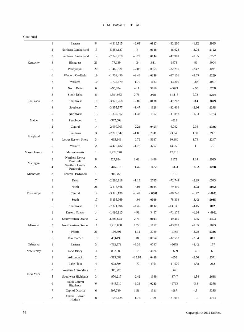
Table A5. Mean difference between times 1 and 2, sample size, t statistic and associated p-value for number of trees and biomass by state and FIA unit for dog-wood in the Eastern United States.

Trees (no.) Biomass (Mg) State FIA unit code Unit name n

Mean of difference1 t2 P3 Mean of difference1 t2 P3

1 Southwest-South 5 –7,605,138 –2.59 .0608 –148,496 –2.5 .0669

2 Southwest-North 7 –16,365,688 –4.66 .0035 –244,723 –3.67 .0105

3 Southeast 21 –4,852,196 –2.69 .0142 –88,654 -2.92 .0084

4 West Central 9 –11,016,959 –3.64 .0066 –188,035 –4.39 .0023

5 North Central 15 –8,454,062 –3.47 .0038 –129,189 –4.5 .0005

Alabama

6 North 10 –6,103,411 –5.75 .0003 –104,343 –4.97 .0008

1 South Delta 9 –942,188 –1.52 .1672 –18,786 –2.01 .0787

2 North Delta 9 –289,672 .75 .4721 59 .02 .9872

3 Southwest 20 –3,676,100 –5.72 <.0001 –36,793 –6.03 <.0001

4 Ouachita 10 –3,613,440 –4.49 .0015 –61,999 –5.5 .0004

Arkansas

5 Ozark 24 –6,968,503 –3.66 .0013 –106,631 –4.68 .0001

Connecticut 1 Connecticut 8 418,917 .84 .4313 –2471 –0.36 .7328

Delaware 1 Delaware 3 –2,181,978 –2.36 .1422 17,634 1.47 .2795

1 Northeastern 12 86,250 .34 .743 –850 –.37 .722

2 Northwestern 14 –965,504 –.98 .3448 –21,616 –1.76 .1012 Florida

3 Central 4 8,360 .01 .9905 515 .16 .8826

1 Southeastern 16 –441,100 –1.6 .1308 –7177 –3.57 .0028

2 Southwestern 16 –907,228 –2.58 .0208 –9543 –2.01 .0629

3 Central 48 –1,525,543 –3.61 .0007 –33,094 –4.95 <.0001

4 North Central 32 –3,609,528 –6.36 <.0001 –48,309 –6.77 <.0001

Georgia

5 Northern 21 –6,245,248 –5.59 <.0001 –66,582 –4.73 .0001

1 Southern 15 779,910 1.65 .1203 –4159 –1.4 .178

2 Claypan 17 –81,072 –.21 .8352 –5404 –1.9 .0754 Illinois

3 Prairie 21 –121,400 –.57 .5769 –2593 –2 .0588

1 Lower Wabash 14 –2,606,899 –2.48 .0277 –21,917 –2.78 .0156

2 Knobs 17 –3,612,894 –5.66 <.0001 –39,490 –6.54 <.0001

3 Upland Flats 8 –184,226 –.57 .5886 –4,392 –1.49 .1806 Indiana

4 Northern 29 3510 .04 .9708 –826 –1.41 .1681

1 Northeastern 1 –420,460 –1259 Iowa

3 Southwestern 1 347,740 309

1 Northeastern 1 –199,955 –284 Kansas

2 Southeastern 2 –59,980 –1.67 .344 –121 –1.37 .4013

Copyright © 2012 SciRes. 51

C. M. OSWALT ET AL.

Continued

1 Eastern 8 –4,316,515 –2.68 .0317 –32,230 –1.12 .2995

2 Northern Cumberland 13 –5,884,127 –4 .0018 –46,023 –3.04 .0102

3 Southern Cumberland 12 –7,240,478 –3.72 .0034 –47,961 –1.95 .0777

4 Bluegrass 23 –77,139 –.24 .811 1974 .86 .4004

5 Pennyroyal 20 –1,466,521 –2.03 .0565 –32,250 –2.47 .0231

6 Western Coalfield 19 –1,759,430 –2.43 .0256 –27,156 –2.53 .0209

Kentucky

7 Western 10 –1,738,479 –1.75 .1133 –13,200 –.87 .4067

1 North Delta 6 –95,374 –.11 .9166 –8623 –.98 .3738

2 South Delta 8 1,584,953 2.76 .028 11,115 2.73 .0294

3 Southwest 10 –3,923,268 –2.89 .0178 –47,262 –3.4 .0079

4 Southeast 7 –3,355,577 –1.47 .1928 –32,609 –2.66 .0375

Louisiana

5 Northwest 13 –1,332,362 –1.37 .1967 –41,892 –1.94 .0763

Maine 3 Penobscot 1 –372,562 –811

2 Central 14 –2,090,903 –2.21 .0453 6,702 2.36 .0346

3 Southern 3 –2,278,547 –1.86 .2041 23,345 1.39 .2991

4 Lower Eastern Shore 3 –635,148 –0.79 .5137 10,380 1.74 .2247 Maryland

5 Western 2 –4,476,482 –1.78 .3257 14,559 1 .5

Massachusetts 1 Massachusetts 1 1,224,278 12,416

3 Northern Lower

Peninsula 8 527,934 1.62 .1486 1172 1.14 .2925

Michigan 4

Southern Lower Peninsula

27 –445,613 –1.49 .1472 –6303 –2.32 .0288

Minnesota 3 Central Hardwood 1 282,382 616

1 Delta 7 –2,290,818 –1.19 .2785 –72,744 –2.39 .0543

2 North 26 –3,415,566 –4.01 .0005 –79,410 –4.28 .0002

3 Central 14 –3,126,130 –3.42 <.0001 –78,748 –6.77 <.0001

4 South 17 –5,155,069 –4.04 .0009 –78,304 –3.42 .0035

Mississippi

5 Southwest 11 –7,371,896 –4.49 .0012 –130,391 –4.15 .002

1 Eastern Ozarks 14 –1,095,115 –.98 .3457 –71,175 –6.84 <.0001

2 Southwestern Ozarks 12 3,803,624 2.74 .0193 –19,465 –1.55 .1493

3 Northwestern Ozarks 11 1,718,808 1.72 .1157 –13,792 –1.35 .2073

4 Prairie 21 –150,491 –1.11 .2789 –1,468 –2.28 .0336

Missouri

5 Riverborder 19 49,619 .18 .8554 –12,553 –3.94 .001

Nebraska 1 Eastern 3 –762,571 –3.35 .0787 –2675 –2.42 .137

New Jersey 1 New Jersey 11 –837,688 –.76 .4626 –8699 –.45 .66

1 Adirondack 2 –315,089 –15.18 .0419 –658 –2.56 .2371

2 Lake Plain 4 –603,804 –.77 .4951 –11,570 –1.38 .262

3 Western Adirondack 1 583,387 867

5 Southwest Highlands 3 –970,217 –2.42 .1369 –8747 –1.54 .2638

6 South-Central

Highlands 6 –845,510 –3.23 .0233 –9733 –2.8 .0378

New York

7 Capitol District 6 597,749 1.51 .1911 –987 –.5 .6385

8 Catskill-Lower

Hudson 8 –1,590,625 –1.72 .129 –21,916 –1.5 .1774

Copyright © 2012 SciRes. 52

C. M. OSWALT ET AL.

Copyright © 2012 SciRes. 53

Continued

1 Coastal Plain 21 –3,117,924 –3.61 .0017 –38,811 –3.62 .0017

2 Northern Coastal

Plain 22 –1,645,716 –4.4 .0003 –21,958 –5.34 <.0001

3 Piedmont 35 –6,349,888 –7.06 <.0001 –83,812 –6.6 <.0001

North Carolina

4 Mountains 21 –11,798,050 –6.53 <.0001 –124,818 –6.07 <.0001

1 South-Central 10 –10,020,912 –3.27 .0097 –92,995 –2.88 .018

2 Southeastern 7 –11,123,902 –2.88 .028 –93,624 –2.25 .0653

3 East-Central 11 –5,534,590 –3.17 .01 –58,209 –3.99 .0026

4 Northeastern 15 –1,689,125 -2.83 .0134 –16,695 –2.75 .0156

5 Southwestern 10 –2,226,981 –1.58 .1482 –29,127 –1.57 .1515

Ohio

6 Northwestern 9 –1,080,125 –1.71 .1248 –5241 –1.15 .2831

0 South Central 9 –2,926,970 –3.4 .0094 –3350 –.7 .5044

5 Western 11 –3,828,340 –2.86 .0171 –33,283 –3.64 .0045

6 North

Central/Allegheny 11 1,466 0 .9987 661 .1 .921

7 Southwestern 5 –4,456,441 –2.26 .0872 –29,428 –2.64 .0576

8 Northeastern/Pocono 12 –975,408 –2.38 .0366 105 .04 .9678

Pennsylvania

9 Southeastern 11 –2,262,721 –3.66 .0044 –20,667 –3.55 .0053

Rhode Island 1 Rhode Island 3 –648,043 –.49 .673 1966 .23 .8402

1 Southern Coastal

Plain 11 –685,049 –.65 .5326 –20,495 –1.54 .1549

2 Northern Coastal

Plain 16 –1,056,274 –2.16 .047 –8,949 –1.25 .2292 South Carolina

3 Piedmont 18 –5,449,847 –3.63 .0021 –80,703 –4.56 .0003

1 West 15 –2,868,802 –3.2 .0064 –53,766 –3.89 .0016

2 West Central 11 –3,545,042 –2.77 .0197 –63,742 –2.8 .019

3 Central 21 –2,261,837 –3.28 .0038 –40,496 –4.33 .0003

4 Plateau 16 –10,654,752 –4.7 .0003 –132,547 –5.21 .0001

Tennessee

5 East 27 –5,506,879 –5 <.0001 –62,323 –6.17 <.0001

1 Southeast 19 –1,751,245 –2.46 .0244 –29,628 –3.48 .0027 Texas

2 Northeast 21 –1,888,624 –3.25 .004 –30,353 –3.45 .0025

1 Coastal Plain 31 –3,140,022 –6.26 <.0001 –25,794 –7.28 <.0001

2 Southern Piedmont 17 –6,315,451 –5.67 <.0001 –54,187 –6.62 <.0001

3 Northern Piedmont 17 –7,343,111 –6.53 <.0001 –52,239 –5.59 <.0001

4 Northern Mountains 14 –9,872,185 –5.61 <.0001 –84,658 –4.84 .0003

Virginia

5 Southern mountains 17 –6,615,961 –8.98 <.0001 –62,655 –6.55 <.0001

2 Northeastern 18 –5,052,487 –5.59 <.001 –31,133 –3.2 .0052

3 Southern 14 –13,888,298 –8.37 <.0001 –85,217 –7.01 <.0001 West Virginia

4 Northwestern 19 –5,058,187 –4.53 .0003 –14,650 –2.3 .0333

1County-level mean difference of the number of dogwood stems > 2.5 cm (1-inch) diameter between times 1 and 2; 2Paired T-test pairing time 1 county-level estimates to time 2 county-level estimates; 3P-value of paired t-test. Bold numerals denotes significance at the .05 level.