an approach to the solution of unsteady unsaturated flow problems in soils
TRANSCRIPT
Department of Civil Engineering
Stanford University
Stanford, Cali fornia
AN APPROACH TO THE SOLUTION
OF UNSTEADY UNSATURATED
FLOW PROBLEMS IN SOILS
by
Flora Chu Wang
Technical Report No. 19
March 1963
Prepared under U.S. public Health Service
Research Grant 1tIP-00246
ABSTRACT
An analytical approach to the solution of unsteady
unsaturated flow problems in soils is presented. In
particular, the method that is developed is applied to
infiltration phenomena. Accordingly, the review of litera
ture covers a number of relevant topics, including, the
distribution of moisture content during downward entry of
water into soils, the general phenomenon of water movement
in porous media, and a recently advanced mathematical theory
of infiltration.
The analytical approaches of Klute (1951), using an
iterative method for solving the flow equation, and Philip
(1957), using the Boltzmann transformation to reduce the
flow equation to an ordinary differential equation, and the
work of other investigators have contributed a great deal
toward the understanding of unsteady unsaturated flow
through sOils. However, the solution of the differential
equation of flow is actually a discipline of mathematics
and has little to do with the physics of the flow problem
In this work an attempt has been made to apply the differ
ential equation of diffusivity in such a way that physical
significance of the phenomena of unsteady unsaturated flo';l
is preserved.
If the hydraulic and capillary characteristics of the
soil are known with a given initial moisture condition, this
new approach, the strip method, permits prediction of the
future disposition of soil moisture as a function of time
and location. The technique is particularly adaptable to
problems of infiltration,_ drainage, and upward flow in soils
induced by evaporation.
Darcy's law is combined with the continuity principle
and based on- a fixed sectlon concept, the equation of flow
is derived. The geometric interpretation of this flow
iii
At!!., " ..• ;u .. 50 Ii<. . _ oS #:=::j::,",-, _~" •••.• ~._.~ .• ,aj!)ia; 'N" _.Wi , _._ ,.x_ Qi::;:'~''''ia; ,zw.u :::ad. L ._d,._ .. i'<,-_r_ 4. '~ .. L\)jDLUi .1& tal H-UJl'I!G, "P"'"

~ ) , l ~
j ;j
~ :if n 1 , 1 J j 1 1 1 1
I ~
i ;
1 i
I /1 II II
II il'
I! i I ~ ! :: i ! i
;1, :1 ;j
, i i r I; d " I : I ;
I ' I I I
II'
equation is also presented. From the viewpoint of geometric
configuration using a concept of moving sections having
fixed moisture content, the solution is achieved through a
step-by-step procedure. The computations are carried out
through use of a digital computer. A numerical solution of
the flow equation for the infiltration phenomenon is given,
and a BALGOL program for this example is also outlined.
This new approach gives results that correspond closely to
the Philip approach. Though at the present stage of develop
ment the method is applicable only to idealized soils, it is
anticipated that further research will lead to the development
of methods permitting application to field conditions.
iv

ACKNOWLEDGMENTS
The writer is especially indebted toProfesBor
Joseph B. Franzini, her thesis adviser, whose help was
invaluable in the preparation of this dissertation. A
number of ideas all. th~ analytical approach were initiated
at the suggestion of Professor Franzini under whose direction
this dissertation was completed. The writer wishes to
express her great appreciation for his guidance. Thanks are
also extended to Professor Norman H ~rawford for his review
of the manuscript. Finally, the writer is indebted to her
husband, Yu Hwa, whose normal support and encouragement
facilitated the development and completion of this project.
Financial support for this research was provided by the U.S.
Public Health Service under Research Grant WP-246.
v

~,," ..
1 ! , ' , ' i: , . . . , , , . ! ; f 1
! ' i, , , I' , , . i; ,
tiN",
Abstract. . . Acknowledgments List of Tables. List of Figures
TABLE OF CONTENTS
Page
iii v viii ix
1. Introduction. 1
2. Review of Literature. 3 2.1 The Distribution of Moisture Content during
Downward Entry of water into Soils--Bodman and Colman's Experimental Observations (1944). 3
2.2 The General Phenomenon of water Movement in Porous Media--K1ute's Equation (1951). 7
2.3 The Mathematical Theory of Infi1tration--Philip's Solution (1957) . 13
3. Description of Unsteady Unsaturated Flow Phenomena. 24 3.1 Idealized Complexities in Unsteady Unsaturated
Flow Phenomena . ..... 24 3.1.1 General Nature of Soil MOisture Tension
or Capillary Head--1/1 = fl(e). 24
3.1.2 Permeability as a Function of Moisture Content--K = f 2(e).. .... 30
3.1.3 Physical Relation for the Energy Gradient - - i = f' -=< ( 1/1 ) . 38
-' 3.2 Natural Soil Characteristics in Unsteady
Unsaturated Flow Phenomena . 43 3.2.1 The Effects of Swelling and Shrinkage
on the Structure of Soils . 43 3.2.2 Non-homogeneity in the Soil Structure 47 3.2.3 Bacterial and Biological Influences on
Soil Structure. . . . . 49 3.2.4 Effect of Chemical Characteristics of
the "later . 50
4. Analytical Approach to the Solution of Unsteady Unsaturated Flow Problems in Soils--Writer's Analytical Work--Strip Method . 4.1 The Nature of Unsteady Unsaturated Flow in
Soils. 4.2 Darcy's Law and Cont.inuity Principle Applied
to Unsteady Unsaturated Flow .
vi
53
56
i. )
)
TABLE OF CONTENTS (Continued)
Page
4.3 Derivation of Differential Equation of Infiltration by Concept of Fixed Section. 57
4.4 Analysis by Strip Method Using Concept of Moving Sections Having Fixed Moisture Contents 62
5. The General Outline of the Numerical Procedure. 5.1 The Basic Data for Illustrative Example ... 5.2 The Numerical Example of Hand Calculations .. 5.3 A BALGOL Program through Use of the Burroughs
220 Digital Computer .......... .
6. Conclusions, Discussions, and Further Research Possibilities ............... . 6.1 Testing the Results of the Strip Method. 6.2 Comments on This New Approach ..... . 6.3 Suggestions for Further Research Possibilities
Appendices A. List of Symbols. . . . . B. Results of Computations. C. Bibliography ..... .
vii
68 68 73
82
96 96 101 104
A-l B-1 C-l

I: " i 1 '"
I j , J 1 j J
, j ~
l ~
J , 1 " 1 1
1 1
j ! 1 ,
i j !
" ': ,
'I',
'"
,
i : I i , , j,j
, " il
; :1 ! :!
LIST OF TABLES
Number Title Page
5.1 Wetting Soil Moisture Tension 1/1 and Permeability K as Functions of Moisture Content e . 69
5·2
5 3
h 4 .-J
') 5
c, 6 -"
6 1
Values of Soil MOisture Tension Permeability K used to compute Yolo Light Clay ..
1/1 and Infiltration Into
Sample Computations of Infiltration Into Yolo Light Clay by Strip Method. 74
Example of BALGOL Program for Infiltration Into Yolo Light Clay. . 84
Numerical Results of Computed Moisture Profiles by the Strip Method . 87
Nurnerical Results of Computed IVIoisture Profiles for Large Times by the Strip Method. 92
Computed Infiltration Rate for Yolo Light Clay by the Strip Method . 97

ill
LIST OF FIGURES
Number Title Page
2.1 Moisture Depth Curves (Bodman and Colman, 1944). 4
2.2 Schematic Representation of MOisture Profile (Bodman and Colman). . . . . . . . . . 5
2.3 Infinitesimal parallelepiped of Medium 7
2.4 Computed Moisture Profiles During Infiltration Into Yolo Light Clay (After Philip 1957a) . . . . . 23
3.1 The Occurrence of Moisture in Soil .
3.2 Diagram of a Soil Column at Moisture Equilibrium with a Free-water Surface ........ '.' .. 25
3.3 Moisture Content versus Height Curves for Typical Soil (After Buckingham 1907) . . . . . . . . . . . 28
3.4 Energy Relations for Greenville Loam (After Schofield 1935) . . . . . . ,
3.5 Permeability as a Function of Capillary Potential
29
K = gl (1/1) (After Moore 1939). . . . . . . . . 32
3.6 Permeability as a Function of Moisture Content K = f 2(6) (After Moore 1939). . . . . . . . . 33
3.7 Ratio of Unsaturated to Saturated Permeability as a Function of Sat'.lration (After Irmay 1954). 35
3.8 Schematic Representation of Relation between Threshold Moisture Content 60 and Inactive
Moisture Content 6 i . . . . . . . .
3.9 Computed Profiles of Total Potential ¢ Infiltration Into Yolo Light Clay
During
3.10
(After Philip 1957d) ...... .
Soil Moisture Tension versus Depth Yolo Light Clay 1/1 = g,,(Z) (After
-'l0
Z Curve for Moore 1939)
3.11 The Corresponding Energy Gradient i in all. Infiltration Situation for Yolo Light Clay
37
40
41
i = f3
(l/1) .•.•. ••••••••••.• 42
ix
i , I · i
I: -"'j : ii. ' q I, ! I': .:
il'l , 1 _,I:: III :: II i ,i " l.t
ii I : Ii; I: .
I I, " !
Ii I: I' i i L I' ,
I ! . L,! ,
l T Ill' , ,I!' Ii;
" I
il" •
LIST OF FIGURES (Continued)
Number Title Page
3.12
3.13
3.14
3.15
If. 1
4.2
4.3
4.4
4.5
5.1
5.2
5.3
5.4
6.1a
6.1b
6.2
The Shrinkage of Soils as a Function of Moisture Content B (After Haines 1923) ....... .
The Alternate Drying and Wetting Curves for a Typical Subsoil (After Haines 1923) ..... .
Pore-Space Relationships in Marshall Silt Loam and Shelby Loam (After Baver, 1932) ..... .
The Electrolyte Concentration of Irrigation Water Required to maintain a Stable Soil Permeability for Varying Degrees of Exchangeable Sodium Saturation (After Quirk and Schofield 1955).
MOisture Distribution During Infiltration.
Infiltration . . . .
Schematic Diagram of MOisture Profile for the Fixed Section During Infiltration. . . . . . .
The Geometrical Interpretation Equation ~B ~(Ki)
LIt = LIz
of Infiltration
Moisture Distribution During Infiltration .
44
48
52
55
61
62
Curve of Soil Moisture Tension ~ versus Moisture Content B for Yolo Light Clay (After Moore 1939) 70
Curve of Permeability K versus Moisture Content B for Yolo Light Clay (After Moore 1939) .. , 71
Computed Moisture Profiles During Infiltration Into Yolo Light Clay . . . . . . . . . . . . .
Computed Moisture Profiles During Infiltration
91
Into Yolo Light Clay for Large Times . . . . 95
Infiltration Rate Curve (After Philip 1957c). 99
Computed Infiltration Rate Curve for Large Times 100
Computed and Plotted Moisture Distributions During Infiltration. . . . . . . . . . . . . 103
LIST OF FIGURES (Continued)
Number Title
6.3 Moisture Movement in Soil During Period of Evaporation . . . . . . . . . . . . . .
xi
Page
105

1. INTRODUCTION
It is possible to encounter a state of static
equilibrium of soil 'water, but such a condition is rare,
and most situations are characterized by fluctuations of
moisture content and ;:;apillarity in the soil. Such fluctua
tions often impose steep gradients of hydraulic energy and
thus produce-;:;':1anges of mOisture profile.· The development
of a moisture profile implies that the soil is in general
unsaturated and the flow unsteady.
There are two broad types of unsteady unsaturated floVi
in soils, one in Vlhicn a section of soil is maintained at
saturation, as for example infiltration and capillary rise;
and the other in Vlhi;:;h the surface is free to dry out
through evaporation. Infiltration is of great importance in
the field of irrigation. For example, it is necessary to
know the rate at Vlhich a given soil profile Vlill admit Vlater
in order to design a furroVi irrigation system that Vlill
operate properly. In the field of hydrology it is of
importance to knoc.; the infiltration capacity of the soil so
that the proportion of rainfall that runs off the surface to
produce surface r'~noff can -Ce determined. Such information
is of value in ~Iater yi.eld and flood control studies.
W.hen inf:'..ltri2.tion ceases, the mOisture profile
development con':·inues. Following this redistribution of
mOisture there may be a lengthy period of surface drying
during Vlhich the profile development is characterized by a
further penetration downward of the Vlater front under the
action of gravity and a movement upVlard to the dry surface
through evaporation. Such movement is sloVi and the time
during which this pheno!TIenon takes place may be long, as
during the EUlTlr.1er fall'::1'11 season characteristic of dry farming.
A quantitative selution for future disposition of soil
mOisture is clearly of importance in the field of irrigation
1

: :
! "
i .. i 'i
for the determination of the carry-over of water from one
season to the next. An understanding of unsteady
unsaturated flow phenomena has important application in the
fields of agronomy, hydrology, and sanitary engineering.
The hydrologist is interested in changes that take
place in the redevelopment of the moisture profile and its
effect on the recovery of infiltration capacity during dry
periods. The phenomenon of capillary rise occurs mostly in
the capillary fringe which is the zone overlying the ground
water table and containing interstices, some of which are
filled with water by capillarity against the force of gravity.
Although the capillary fringe is of no particular signifi
cance in large earth dams, it is of great importance in
earth models of earth dams, where the material is fine
enough to be subject to a considerable depth of capillarity.
The capillary fringe is a continuation of the zone of satura
tion and is of importance to the hydrologist in his study of
the hydrologic cycle as it serves as mechanism for the
intake, transport, and return of underground waters to the
surface and the atmosphere.
In the field of sanitary engineering, if one desires to
install a sewage-disposal system without endangering the
safety of any domestic water supply, an understanding of
Lmderground flow is necessary. In some instances the system
may consist of a septic tank with effluent discharging
directly into a subsurface disposal field. Under such
conditions the flow is often unsaturated and unsteady on
which the problem under consideration bears directly.
2

2. REVIEW OF LITERATURE
It should be mentioned that in compiling the review of
literature, the main aim has been to cover those articles
and papers which have a direct bearing on the problem under
consideration, rather than to cover all aspects of unsteady
unsaturated flow and current hydrologic techniques dealing
with the phenomenon. The literature review deals with the
distribution of moisture content during downward entry of
water into soils (Bodman and Colman, 1944), and then the
general phenomenon of water movement in porous media (Klute,
1951), and later, the mathematical theory of infiltration
(Philip, 1957).
2.1 THE DISTRIBUTION OF MOISTURE CONTENT DURING DOWNWARD ENTRY OF WATER INTO SOILS--BODMAN AND COLMAN'S EXPERIMENTAL OBSERVATIONS (1944)
The conditions within the soil of priority interest
have been the distribution of moisture contents and moisture
potentials during downward penetration of water. The
classical experiment in this fi.eld was that made by Bodman
and Colman (1944). In their tests they considered two
initially dry soils, Yolo sandy loam, and Yolo silt loam,
and maintained a constant depth of water (5mm) on the surface
during the test.
The moisture depth curves for the two soils tested are
gi ven in Figure 2.1. The soils differed wid·ely in texture
with accordingly large variations in the time required for
the profile to reach any given level. However there are
also marked similarities in the two curves.
Bodman and Colman divided the wetted zones into the
following distinct parts:
3

~)
Soil Moisture Per Cent by: Weight
Q Ip 27 .,~ " 0 0 10 20 0 [ ::t
0 - #~ 0
minutes
10 10 76 ~ ~ 0 UJ 0 ·M H -rl .j.J ill .j.J
Cti .j.J Cti H ill 280 H ~ "' 20 ~
20 .j.J ·M .j.J Cti .j.J Cti UJ ~ UJ
>0 ill >0 H ·9 Ql 0 H ill '0 CJ '0 CJ
0' Cti ~ Cti ill 0, ·M P.
30 H UJ 30 H UJ ·M ill .r: ·M .-r; H Ql .j.J .-r; ill
B H P. H 0 Q) 0 rJJ p., A p., ·M
0 so 1020
~O 40
(a) Yolo Sandy Loam (b) Yolo Silt Loam
Figure 2.1 MOisture Depth Curves
(Bodman and Colman, 1944)
(a) The surface 1 cm layer of each soil reaches a
moisture content approaching pore space saturation
by the time water has penetrated to a depth of
10 cm.
(b) Below this saturated surface layer, the soil
moisture decreases rapidly with depth to about
5 cm from the surface.
(c) Under the zone described in (b) the mOisture
content decreases with depth until dry soil is
reached.

()
Moisture Content e
TRANSITION ZONE
LRANSMISSION ZONE
N
WETTING ZONE
Front
Figure 2.2 Schematic Representation of Moisture
Profile (Bodman and Colman)
Through a synthesIs of' trieir.observations J the moisture
profiles may be defirled as fiVe distinguished zones which
are represented schematically in Figure 2.2.
(a) The Saturated Zone: Below the soil surface there
is a thin layer ,)1' presumed saturation in which
the moisture content is approaching pore space
s.aturation.
(b) The Transition Zone: .Below the saturated surface
layer. t~e soil moisture decreases rapidly with
depth. untLc it reaches a value little higher than
halfway between the moisture equivalent and pore
space saturation. Moisture eqUivalent is used to

i !
, . !
!- ::
j;. !
j" d , ,
represent the water retained in a soil sample when
subjected to an arbitrary centrifugal force.
(c) The Transmission Zone: Below the zone described
in (b), the moisture content decreases slowly with
both depth and time.
(d) The Wetting Zone: A region of fairly rapid
change of moisture content both with respect to
depth and time.
(e) The Wet Front: A region of very steep mOisture
gradient which represents the visible limit of
moisture penetration into the soil column.
Recent research by Philip, Gardner, Nielsen and others
indicates that there is strong likelihood that the so called
"transition zone" is non-existent. Experimental work in
which soil moisture was measured using a gamma source showed
no sudden drop-off in mOisture content below the soil
surface.
6

2.2 THE GENERAL PHENOMENON OF WATER 1110VEMENT IN POROUS
MEDIA KLUTE'S EQUATION (1951)
By use of the equation df continuity and Darcy's lav.',
Klute (19:',1) der:Lved explicitly the equation of flow
through porous mec'_ia.
Assuming the medium is incompressible, the continuity
equation for flow through a homogeneous medium as shown 1n
Figure 2.3 is
~-clt -
o(pv) o(pv) x y - ----OX- - dy dZ
A 2. I
J!---/-- P v ~. A
x
Figure 2 3 Infinitesimal Parallelepiped of Medium
7

.)
", )
.. '!
where p' is the mass of fluid per total volume, p is the
fluid density and v is the volume flux of fluid, that is,
the volume of fluid flowing through unit cross section per
unit time. Expressed in vectorial form,
~ Clt . = - di v (pv) = -\7'(pv)
Darcy's law for the motion of water in a porous
system is
v = - KYrp
where - \7rp is the negative gradient of the total
moisture potential, and K is the permeability.
Substituting Eq. (2.2) into Eq. (2.1) yields
~ Clt = \7' ( pKYrp) =
(2.1 )
( 2.2)
( 2.3)
where p is the porosity of the medium. If the medium is
saturated with water (p' = constant) and since water is
incompressible, (p = constant), Eq. 2.3 can be expressed as:
\7 . ( KYrp) = 0 ( 2.4)
This is the general equation for the flow of water through
a saturated medium.
For an unsaturated porous medium, not all of the void
space is filled with water, therefore Eq. (2.3) can be
written as
= \7. ( pKYrp )
8

where Ps is the bulk density on a dry weight basis,
Mass of Solid Ps = Total Volume
Dry Weight of Soil = (g) (Total Volume)
and Bs is the mOisture content on a dry weight basis,
Weight of Wat.er Bs- Dry Weight of Soil
This leads to
= Dry Weight of Soil . Weight of Water ( g) (Total Volume) x Dry Weight of Soil
J"Iass of Water = Total Volume = pi
If B is defined as the moisture content expressed in
volumetric terms
B =
then
Volume of Water Total Volume
Mass of Water Volume of Water pB = Volume of Water x Tot.al Volume
that. is
Hence Eq. (2.5) can be written as
9
--~---~ ----
Mass of Water = ;;;;Tc='o7t-=a'"1-"-"V"'o"';1i-:u'-m'-e'-'- = p I

, .
j
Ii .. j:
I;(~' !:1' J
j, ~
~~:-
~\-~ ,
-'j"
".It:
iii
1!"
:ii
.Ij
d(pe) dt =
and with p a constant this yields
de 1 dt = 'V' ( KVCP ) (2.6)
This is the general equation for the flow of water through
an Lffisaturated porous medium.
The total pot.ential cP is considered as the sum of
the negative pressure (capillary potential) 1/J , and the
gravitational potential Z which is positive upward. For
flow in a vertical column of the medium,
If 1/J and K are regarded as single~valued functions
of e,
= 'V' (K'V1/J+K)
Hence,
1 This equation was originally developed by Richards, L. A., Capillary Conduction of Liquids in porous medium, physics 1: 318-333, 1931.
10
)
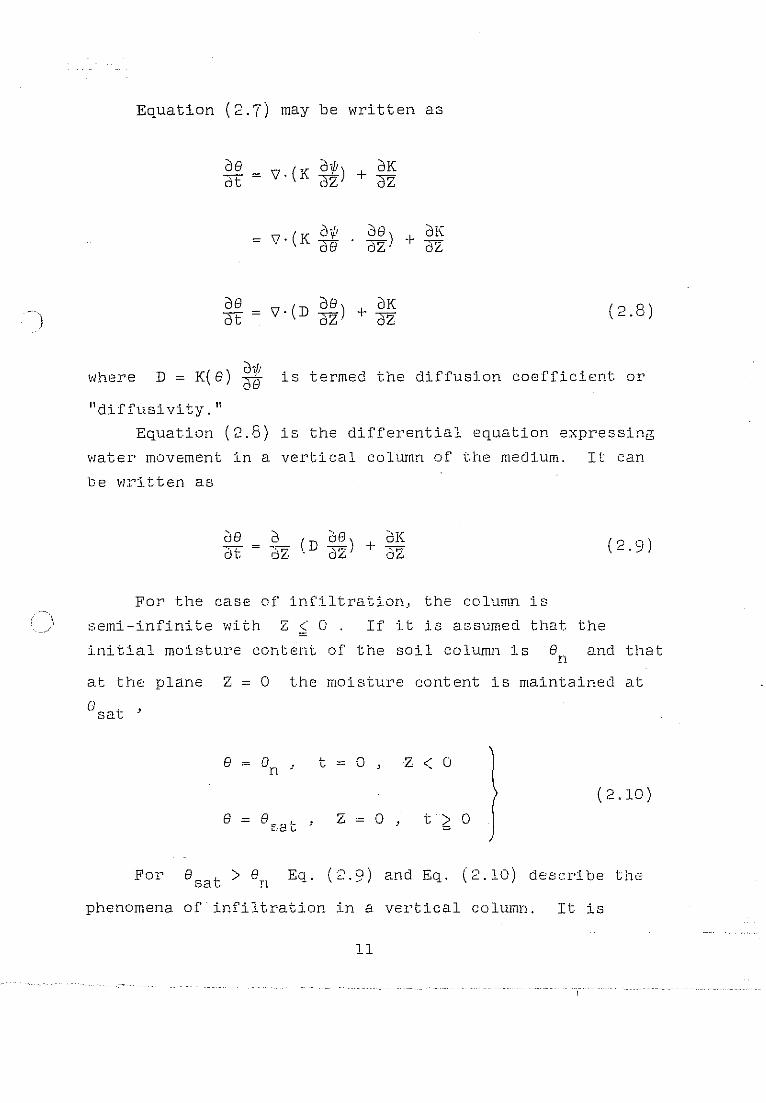
Equation (2.7) may be written as
oB n (K ow) + oK dE" = V' cz dZ
(K 21~' OB) + oK ="iJ' dB' dZ dZ
~Bt = "iJ'(D~) + ~ u oZ oZ (2.8)
where D = K( e) d~J is termed the diffusi.on coefficient or dB "diffusivity."
Equation (2.8) is the differential equation expressing
water movement in a vertical column of t.he medium. It can
be written as
dB dt
(D d~) + oK . dL. 6Z (2.9)
For the case of infiltration., the column is
semi-infinite with Z < O. If it is assumed that the
initial moisture content of the soil column is Bn 2nd that
at the plane Z = 0 the mOisture content is maintained at
B - Bn , t = o. Z < 0
(2.10)
B = B.a.' Z - 0 ,-, L..
t ;; 0
For Bsat> en Eq. (2.9) and Eq. (2.10) describe the
phenomena of infiltration in a vertical column. It is
11

..; I'r ; : .',. II" !;il :;g .L ;
convenient to write x for (-Z) , so that Eq. (2.9) and
Eq. (2.10) become
dB d (D dB) dK Cit = ax - dX .ax (2.11)
B = B , t n = 0 , x> 0
(2.12)
B = Bsat , x = 0 , t ~ 0
x is now the vertical ordinate, positive downward, hence
the region to be considered is positive. Equation (2.11)
is a non-linear, second order partial differential equation
of the diffusion type, inhomogeneous in B
Klute suggested a numerical method of solving Eq. (2.11).
However, Philip in reviewing this method found the accuracy
to be poor even with considerable labor expended.
Subsequently Philip (1957) developed a new numerical
procedure which enables a rapid and accurate solution of
Eq. (2 .ll).
12

2.3 THE MATHEr-1NI'ICAL THEORY OF INFILTRATION --PHILIP'S
SOLUTION (19~'7)
A summary (:f Lhe method a::: 0utliEed by Philip (19';7) i;,
p:iven belovJ.
The equation fc'r ini"i.ltrBtion as ExpresGed by Klute viafJ
subject to the conditions
e _. rJ n
9 = D . sat. "
dK (2.11) - -,-~JZ
x - 0 .' t 2; 0
As a first estimate of x, Philip dropped ehe last
'cerm of Eq. (2.11) and worked v;1th the non-linear diffuE!ion
equation for the case Gf' horlzontal infiltration
where x' is a first estimate of x. Eq. (2.13) is
rmbJect to the conditions,
B f) n
, t - 0 x, > 0 ~ 9 = ro
CI [:Ia t , Xl = 0 , t 2; 0 !
13
(2.13)
(2.14)
.---.--.~

, ~, I :11
l j!
! 1,: I:" , ;!
') , :, ~ Ji
"
.~ 0",
-!:~
;:j
i.m Hn ! ~!: 1m
),; i III
,i· , n' !, i 1!
IT" ::'
" " Ii ,I
" ![ H' " ~i
5 1 ii II
~ ,I ]
ii "
!
The transformation
q, ( e) = x't
1 oq, - 2 (liT = t
1 - 2
( 2.15)
allows Eq. (2.13) to be reduced to the ordinary differential
equation
__ (oD oe fd(f) d(f)-
2 2 D ~) (oq, )
dq,2 ox'
( q, -1 de d -~ t ) d(f) = d(f)
1 2 (D ~)(t- 2)

" ....
(2.16 )
and e is then made the independent variable by multiplying
both sides of Eq. (2.16) by giving
subject to the conditions
e ->- e , <p ->- 00 (this implies that n
e = e sat ' <p = 0
Integrating leads to
<p de = - 2D
e e de ->- 0) ->- n' d<p
= 2D de d<p
( 2.17)
(2.18)
(2.19)
The lower limit of the integral is fixed as en by Eq.
(2.18), therefore Eq. (2.19) is subject to the condition
e = e sat ' <p = 0 (2.20)
Equation (2.19) subject to Eq. (2.20) is then solved
by means of forward integration with one initial condition
determined by trial and improved by iteration. Full details
of the method are given in one of Philip's earlier papers l
1
• 44 ·
Philip, J. R., Numerical solution of equations of the diffusion type with diffusivity concentration-dependent. Trans. Faraday Soc., 51, pp. 885-892, 1955.
15
j. ,
i 'I 1 , I ,
,,'
i j .: I ,
rrn= 75
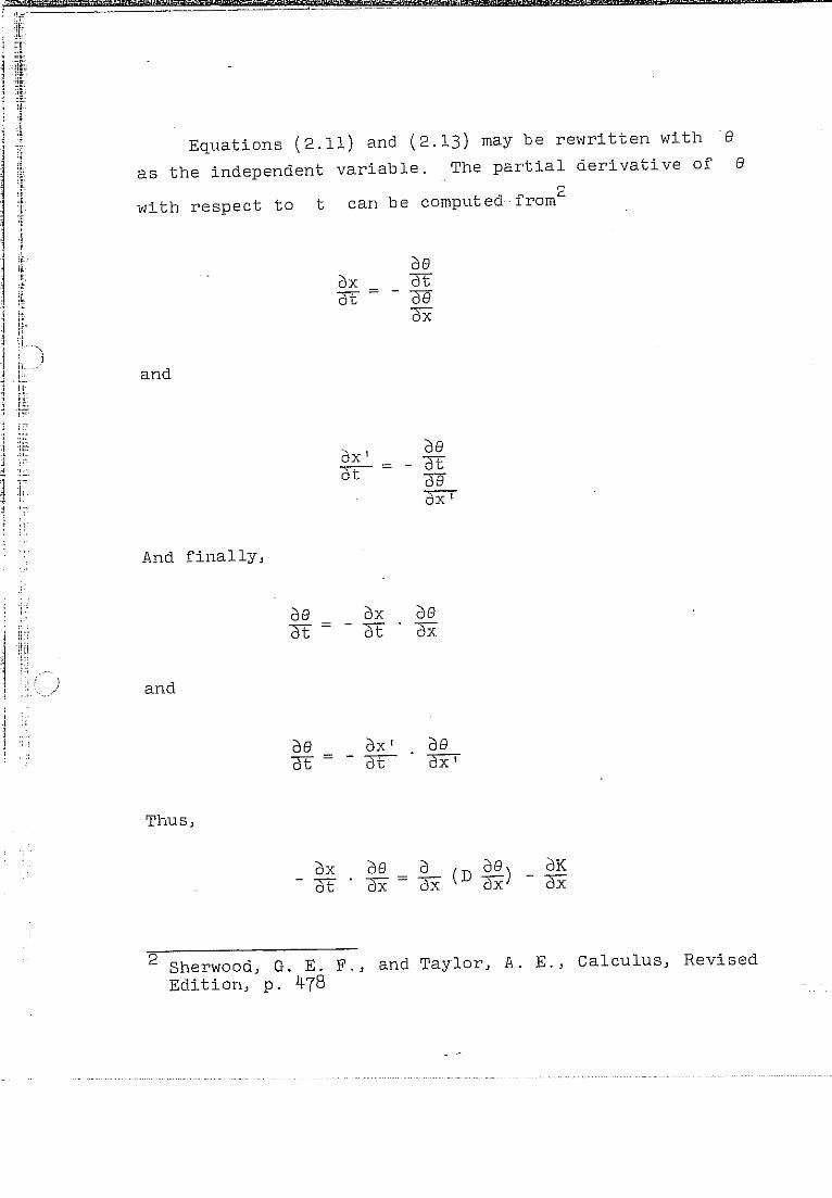
Equations (2.11) and (2.13) may be rewritten with e as the independent variable. The partial derivative of e
with respect to t can be computed from"
and
And finally,
and
Thus,
ox - Cit
dX' at
de = - Cit
de ox'
de dx =
2 Sherwood, G. E. F., and Taylor, A. E., Calculus, Revised Edition, p. 478

and
dX' de d (D de ) - dt dX' = dX' dX'
Multiplying both sides by
Philip obtained
dX de and
dX d (de dK - ot = dB D CiX) - dB
and
dX' dB
Subtracting Eq. (2.21) from Eq. (2.22)
respectively,
(2.21)
( 2.22)
%t (x-x') = ~ (D ~~,(¥X _ %~')) + ~~
where
dy _ d (D ~~) + dK dt - dB clx' OX dB
y = x - x'
the approximation
applied to Eq. (2.23), leads to
17
(2.23)
(2.24)
(2.25 )

.,
,u,. t,~, .
nHi)
~'.
'" " " 1:'
i: i'
Eq. (2.26)
written as
cannot give y exactly, hence y
y' , the first estimate of y
~ 0 ( oe oy' oe + oK o~ = OS D OX' dB dxT) OS
Use of the transformation
x(e) = Y't- l
y' = Xt
(2.26) .
should be
(2.27)
( 2.28)
enables Eq. (2.27) to be reduced to the ordinary differential
equation
1 2
X = ~ (D (~t- 2) ¥e t) + ~
d ( (de)2dX)+dK X = a:e D diP diP ae
X = ~e (p(e)~) + ~~ (2.29)
in which

~)
pte) = D (~:) 2
Integrating Eq. (2.29), gives
fe
X de = pte) ~ + (K - Kn) e,
n
(2.30)
(2.31)
in which Kn is written for th.e value of K at e = en
subject to the condition
X = 0
Again, Eq. (2.31) subject to Eq. (2.32) is solved
numerically with same method as before.
The new residual error
(2.32)
is then introduced. The same procedure may be repeated with
new residuals until the necessary accuracy is attained.
The solution of Eq. (2.11) is thus found as a power 1
series in
since
2' t ,
",(e)
x( e)
7/1(e)
=
=
=
1 -2 x't
y 't'l
3 - r;
zit c:
1 2
, X, ",(e)t
, y' = x(e)t 3 2
Zl 7/1(e)t =
19

and
so that
That is,
I
x = ¢(e)t2 + x(e)t +
y = x - x'
z = y - y'
x = x' + y
= x' + y'
= x' + y'
3
+ z
+ Zl
~(e)t2 + m(e)t2 + ___ +
.. . .
m
f m(e)t 2 + ---
(2.33)
in which the coefficients ¢(e) , x(e) , ~(e), m(e) , .. , ~ f (e) are functions of e which are the solutions m
of a series of ordinary differential equations which can be
solved by simple numerical methods.
The total infiltration F may be readily obtained
since the total change of moisture content in the semi
infinite column equals the difference between the time
integral of the flux at x = 0 and at infinity
x de + Knt (2.34)
Integrating Eq. (2.33) with respect to e
20

(
m
+ t~~ (e) + ---m
( 2.35)
",here the notation J f(e)
J esat
denotes f(e) de .
en
The series of Eq. (2.35) converges for all expect very
large t) which case has been dealt with by an alternative
method involving a different approach (Philip 19'::;7c). Then
using Eq. (2.35) in Eq. (2.34)
+ t:J + --(l)
m
+ t2~ (e) + ---m
(2.36)
If the infiltration capacity is denoted by l' (that is the
-flux at x = 0) ) then
l' = dF
= :I,t 2 2% + --- +
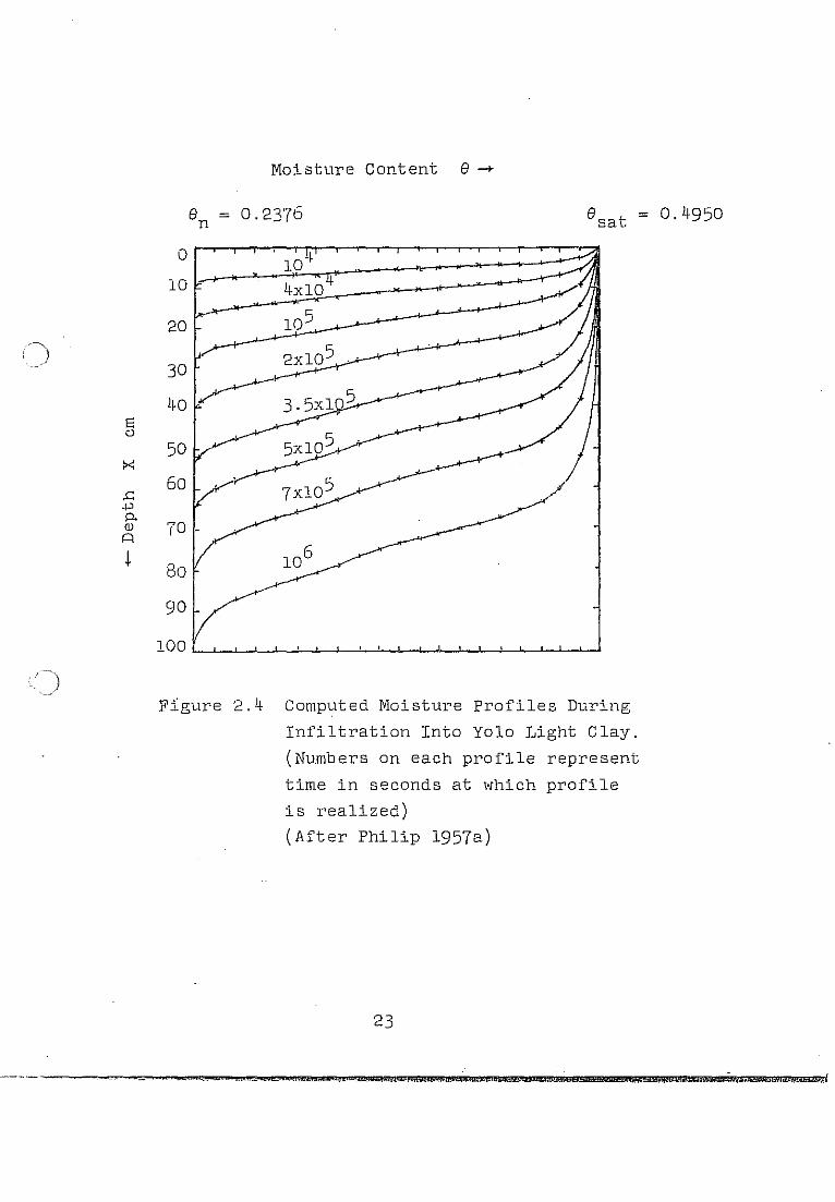
The results obtained by using the foregoing procedure
can perhaps best be noted by citing in brief the numerical
example given by Philip (1957a). The problem is that of
21
P @?4MW 946b I/WjH itlumJi@

infiltration into Yolo light clay with an initial gravimetric
moisture content of 18;'b. On a volume basis 8n = 0.2376
since the apparent specific gravity of the soil was 1.32.
At the plane x = 0, 8 is maintained at its saturation
value of ~-( ~/~ (8 = 0.4950). -' ,./ sat
In the language of this section the problem reduces to
solving Eq. (2.11)
(D (8) _ CiK dX ax
subject to Eq. (2.12) with
e = Bn = 0.2376 J t 0, x > 0
8 = 8 t = 0.4950, x = 0, t > __ 0 ~a
'l'he diffusion coeffi cient D and the permeabi li ty K were
derived by Philip from de.ta by Moore (1939). 'Figure 2.4
shows the results for t = 0 to t = 106 seconds, each
curve represents a rr.oiE-ture profile at a particular time
during infiltration.
22
s ()
:x:
.c: ..., P. ill r::1
t
Moisture content S->-
Sn = 0.2376 S sat =
0 10+ 10 4xlO
" 20 10:';
30
40
50 5xl05
60
~ 80
90
100 . ,
Figure 2.4 Computed Moisture Profiles During
Infiltration Into Yolo Light Clay.
(Numbers on each profile represent
time in seconds at which profile
is realized)
(After Philip 1957a)
23
_. <Q _ 'z _. ~_ ii4 ( .,AWlJl_ ;::; 45.,
0.4950
3.1
m"''TCt'M''''eD'Q';:H" Maw
3. DESCRIPTION OF UNSTEADY UNSATURATED
FLOW PHENOMENA
IDEALIZED COMPLEXITIES IN UNSTEADY UNSATURATED
FLOW PHENOMENA
3.1.1 GENERAL NATURE OF SOIL MOISTURE TENSION OR CAPILLARY
HEAD--1fJ = f l (8)
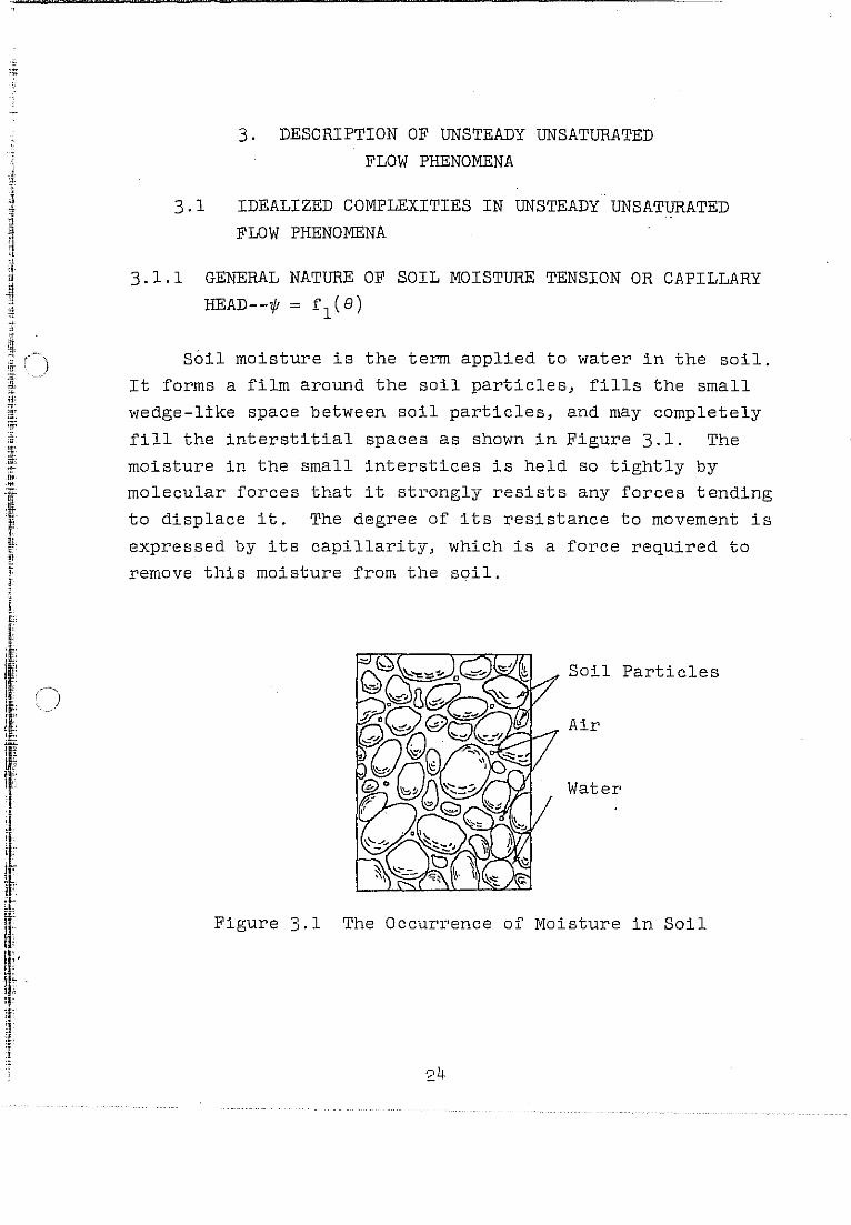
Soil moisture is the term applied to water in the soil.
It forms a film around the soil particles, fills the small
wedge-like space between soil particles, and may completely
fill the interstitial spaces as shown in Figure 3.1. The
moisture in the small interstices is held so tightly by
molecular forces that it strongly resists any forces tending
to displace it. The degree of its resistance to movement is
expressed by its capillarity, which is a force required to
remove this moisture from the soil.
Soil Particles
Air
Water
Figure 3.1 The Occurrence of Moisture in Soil

Buckingham (1907) first proposed characterizing soil
moisture phenomenon on the basis of an energy relationship.
He visualized the flow of water through soil as being
comparable to the flow of electricity through a conductor
and introduced the term capillary potential ~ (analogous
to electric potential) to describe the attraction of soil
for water. Capillary potential ~ is the potential energy
per unit mass o~f water, and it is defined as the work
required to move a unit mass of water from the free-water
surface to the specified point, against capillary force in
the column of soil. It will be seen that, capillary
potential is negative in sign, since water will move upward
from groundwater by capillarity, and work is required to
move water in the soil downward to the reference plane
against capillary action.
'=.:::;::=-- ~-----------_ .....
Figure 3.2 Diagram of a Soil Column at Moisture
Equilibril@ with a Free-Water Surface
25
)
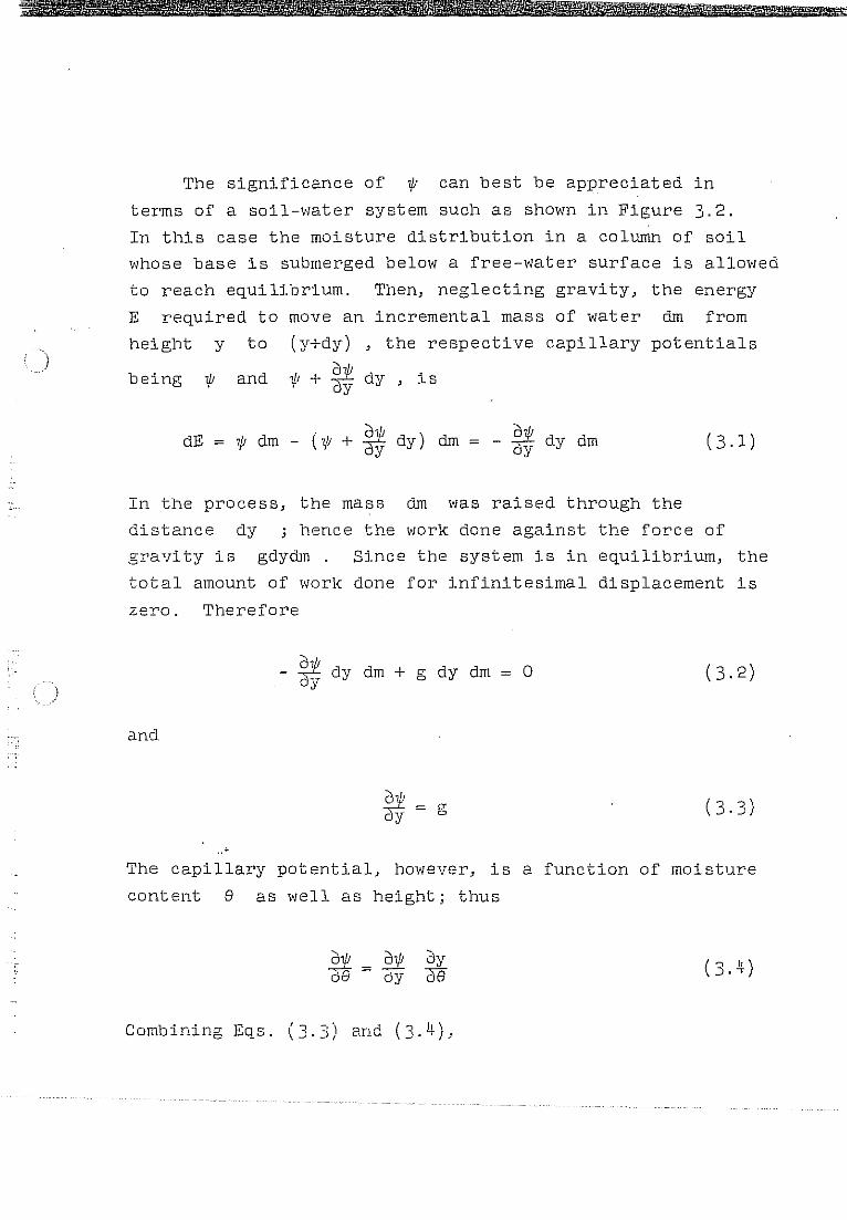
The significance of * can best be appreciated in
terms of a soil-water system such as shown in Figure 3.2. In this case the moisture distribution in a column of soil
whose base is submerged below a free-water surface is allowed
to reach equilibrium. Then, neglecting gravity, the energy
E required to move an incremental mass of water dm from
height y to (y+dy) , the respective capillary potentials
being ~I and 1/1 + %t dy , is
dE = * dm - (1/1 + ~ dy) dm = - ~ dy dm (3.1)
In the process, the mass dm was raised through the
distance dy ; hence the work done against the force of
gravity is gdydm. Since the system is in equilibrium, the
total amount of work done for infinitesimal displacement is
zero. Therefore
and
~' - . dy dm + g dy dm = 0 y
d1J; - = g dy
(3.2)
The capillary potential, however, is a function of moisture
content e as well as height; thus
(3.4)
Combining Eqs. (3.3) and (3.4),

)
d1/1e
= dY dB gdB (3.5)
Integration of either Eq. (3.3) or (3.5) yields (noting that
1/1 = 0 when y = 0)
1/1 = g y (3.6)
Consequently, the capillary potential 1/1 in the c.g.s.
system of units, is numerically equal to the hydrostatic
pressure of the soil water. In unsaturated soils the hydro
static pressures are negative and are frequently replaced by
positive values called soil moisture tensions which are
expressed in terms of the height of a liquid column required
to produce them. That is, their values are negative with
respect to atmospheric pressure, and are usually expressed
in centimeters of water. When the absolute value of the
soil moisture tension is less than one atmosphere ~t may be
determined by means of a tensiometer. For greater tension
its value may be determined by means of a centrifuge or
pressure extractol". Buckingham made numerous experiments
with soil columns and found the relation between soil moisrure
) tension and moisture content. His investigations showed that
the energy required to remove water from soil is a continuous
function, and with moisture content at corresponding Deights
being greater for finer soils as shown in Figure 3.3.
Schofieldl (1935) suggested the use of the logarithm
of the capillary potential pF to express energy relations
of soil water. He defined pF as the common logarithm of
the head in centimeters of water necessary to produce the
1 Schofield, R. K., The pF of the water in Soil, Trans. Third Intern. Congr. Soil Sci., Vol. 2: 37-48, 1935
27

)
40 H ill ...,
30 ctI rIl ~ ill
.c: ill "
Sandy Loam Cecil Clay :> ~ 20 0 H .g ~
·rl ..., 10 .c: rl bO ill ·rl ill ~
:> 0 ill 10 1 H 2 22
Moisture Content in percent
Figure 3.3 Moisture Content versus Height Curves
for Typical Soil (After Buckingham 1907)
soil moisture tension corresponding to that capillary
potential, and thus reduced the extreme range in the values
of the potential facilitating graphical presentation.
Figure 3.4 shows the relation between pF and moisture
content for Greenville loam. It will be noted that a series
of experimental data cannot be expected to plot on a single
curve because there is a marked hysteresis; the value of
soil moisture tension is different depending upon whether
the soil is being subjected to wetting or drying. It is
considerably lower during wetting than during drying. Also,
the lower the moisture content, the greater the soil moisture
tension. Because of this hysteresis phenonomenon one must
be careful to use correct curve when dealing with soil
moisture tensions.
28

7 10,000,000
6 1,000,000
') 100,000
~. 10,000
'" 0. 3 1,000
, 2 , , 100 ,
\ \
1 10
0 0 10 20 3 :; 1
Soil Moisture content e Figure 3.4 Energy Relations for Greenville Loam
(After Schofield 1935)
29
¥ .LzD¥!JWLE&
~ u
-;;>-
.:: 0 'M [}J
;::: QJ
I:-< (jJ
H ;::I
.J-l DO
'M 0 :;;: rl 'M 0 (/)

.. :1
.. , .!
!<;; '" ;
)
rmnwm:: '=tWGnmzm '= 2 m 7="
3.1.2 PERJ>1EABILITY AS A FUNCTION OF MOISTURE CONTENT-
K = f2
(e)
The introduction of the capillary potential function
gave rise to the study of soil moisture as a dynamic system.
By applying this concept to soil moisture studies, the
velocity of flow of water through the soil is considered to
be proportional to the total water-moving force. A conduc
tivity factor, variously called capillary conductivity,
conductivity, and permeability, has been used to express
this proportionality. The term "permeability" is adopted in
this dissertation.
Many data on the permeability of soils in saturated
flow, or with the void spaces entirely filled with water,
are available in papeis of the U.S. Geological Survey and
the American Geophysical Union. However, there are rela
tively few published data on soil permeability in unsaturated
flow. In an unsaturated soil a portion of the void space is
filled with air. This reduces the volume of the medium that
is available for the flow of water. Hence the permeability
of an unsaturated soil depends on the moisture content.
Moore (1939) carried out experiments in which water
moved up a soil column from a water table to be evaporated
from the surface into a controlled atmosphere. At steady
state conditions when the rate of water uptake and the
capillary potential throughout a soil column became steady,
the moisture profile provided all degrees of saturation down
to the almost dry surface soil. The mOisture profile was
determined by direct sampling and the capillary potential by
tensiometers. A knowledge of the capillary potential
together with the rate of flow permitted the permeability to
be evaluated from Darcy's equation at each point in the
profile of k..'l.own moisture content.
30

)
Darcy's law for the motion of water in a porous system
is
v = -Kv¢ (3.7)
That is, the velocity of flow v, may be expressed as the
product of K, the permeability of the soil to water, and
(-v¢) , the total potential gradient tending to cause flow.
For the upward·movement of water in an unsaturated soil
column, (-v¢) is composed of the gradients of capillary
potential *, and of the gravitational potential Z,
therefore
v¢ = vt + 1 (3.8)
Combining Eqs. (3.7) and (3.8), gives
v K = -(vt + 1)
According to Eq. (3.9), unsaturated permeability may be
investigated as a function of capillary potential *, that
is, K = gl(t) . K could also be studied as a function of
mOisture content e through the relationship between t and e , that iS J t = fl(e) as given in Section 3·1.1.
The functions of K = gl(t) , and K = f 2 (e) are shown in
Figure 3.5 and 3.6 respectively.
Irmayl (1954) theOl"ized that the permeability K of
unsaturated soil is not constant, but a universal function
of the degree of liquid saturation. An
1 Irmay, S., On the Hydraulic Conductivity of Unsaturated Soil, Trans. Amer. Geophys. Union, Vol. 35: 463-467, 1954
31
'"FA 4A4& = =

)
14 , ,
12 Yolo Light Clay
e.) 10 OJ rIl
"-s 8 l-e.)
'0 0 rl
:2 6
?oo -I-' 4 ·rl rl orl .0 ttl 2 OJ
~ OJ P. 0
, ~L
-600 -500 -400 -300 -200 -100 0
Capillary Potential 1/1 cm
Figure 3.5 Permeability as a Function of Capillary
Potential K = gl(1/1) (After Moore 1939)
32

14
"., 12 Yolo Light Clay
) C)
OJ [J]
"'-S 10 C)
'-0 0 r-! 8 Q ;>, 6 +' ." rI ." .0 4 cd OJ
~ OJ 2 p,
0 14 18 22 26 30 34 38 42
Moisture Content B (by '<Ieight)
Figure 3.6 Permeability as a Function of Moisture
Content K = f 2(B) (After Moore 1939)
33

approximate theory gives the form, which is a cubic
parabola, and it can be expressed by
K = -y Cd 2 I.L e 2 - p)
(3.10 )
where -y is unit weight of the fluid; I.L is dynamic
viscosity of the flui.d; C is a constant which equals
approximately 0.01, depending on the shape of grains and the
soil structure; de is the effective grain diameter; 8 is
the degree of saturation; 80 is the threshold saturation,
being that part of the voids which is filled with non-moving
water; and p is the porosity. More specifically,
.)
p.J -(--~ .::. - PI
(3.ll)
where Ksat is the soil permeability to water under
conditions of complete saturation. The ratio of Eqs. (3.10)
to (3.11) will be
(3.12)
The curve for K/K _to Sa
plotted against 8 is shown in
Figure 3.7 for 80 = 0.20. 8ince the degree of saturation,
8 , is defined as
8 = e p (3.13)

where S is the volume of water in a unit volume of soil;
and p porosity, is the volume of voids in a unit volume of
soil. Therefore Eq. (3.12) can be written as
(
S-K = Ksat S
sat (3. l~)
Where SiS are the various moisture contents on a
volumetric basis; and So is the threshold moisture content.
The writer has tested some of the available experimental
data and there are indications that a value of 4 or 5 for
the exponent of Eq. (3.1~) is more appropriate. However,
this is based only on the empirical form without any
theoretical justification.
~I} 1.0
0.8 0 ·rl +-'
0.6 ttl ~
:>, +-' 0.4 ·rl rI -rl
~ 0.2 OJ e OJ 0 P.
0 0.2 0.4 0.6 0.8 1.0
Degree of Saturation S
Figure 3.7 Ratio of Unsaturated to Saturated
Permeability as a Function of
Saturation (After Irmay 1954)
35
,0; =0. __ a aow .• CQliG&iM<W e:nJjZQJ\;;zz:£gtM4kS t i@l:::z;ltt$j"Ue

In this discussion of the permeability as a function of
moisture content, two of moisture contents requring defini
tions are the threshold moisture content eO and the
inactive moisture content ei . The threshold moisture
content eO is defined as the moisture content below which
liquid film continuum in the soil no longer exists. If the
moisture content is less than eO only vapor movement
through the soil can occur. In this dissertation we are
restricting ourselves to isothermal, liquid phase movement,
hence there is no vapor movement. The inactive moisture
content ei is defined as that moisture which does not
contribute to the flow through the soil. It consists of
hygroscopic moisture absorbed at the surface of the soil
particles and some of the capillary moisture held in the very
fine interstices. It is essentially inactive and will not
flow through the soil under the hydraulic energy gradients
that are ordinarily encountered. For most soils the inactive
soil moisture ei is not constant. It tends to decrease
somewhat in value as the moisture content e of the soil
gets larger than eo The relationship is represented
schematically in Figure 3.B. This phenomenon is created by
the unbalance in molecular forces that occur as the liquid
films in contact with the soil particles get thicker.
Threshold moisture content eO is a constant for a given
soil. It represents the lowest mOisture content at which a
soil exhibits permeability. At threshold mOisture content
all moisture is inactive. At higher mOisture contents ei
becomes somewhat smaller than eO However, for most
instances it may be assumed that ei is approximately equal
to eO over the full range of moisture contents. This is 'a

very good approximation for sandy soils though not very
good for clays.
CD
-IJ ~ ill
-IJ ~ 0 0
ill H ;:)
-IJ rn .r! 0 ~
-IJ ctl rJ)
CD
CD
0 CD
Air Content
" .,.-_---i>i<80 8. "" C ,[sat; Vapor Liquid Phase Mov8J1ent
JYiJvemerrt
Moisture Content e--Figure 3.8 Schematic Representation of Relation
between Threshold MOisture Content 80 and Inactive Moisture Content 8i
37
== .''"''E! Law emmA!

()
3.1.3 PHYSICAL RELATION FOR THE ENERGY GRADIENT--i = L,(ljJ) :)
The energy concept of soil moisture has been shown to
be useful in problems of moisture flow. Since all flow
phenomena are the consequence of an energy gradient, some
method of evaluating the potential energy at various points
in the system is needed if the flow is to be characterized.
In an unsaturated soil, disregarding the effect of gravity,
the velocity of flow is proportional to the difference in
capillary potential, and water tends to flow from the
moister regions of the soil to dryer regions. In other
words, the direction of flow is from a region of high
potential to a region of low potential. When expressed in
terms of tension, flow will occur from regions of low tension
to regions of high tension.
Moisture movements are influenced by the force of
gravity in addition to the capillary force. The sum of the
energy gradients of capillary potential ~ and gravitational
potential Z is the total force affecting vertical moisture
movement. The energy gradient i is expressible in a
variety of forms depending on the nature of the flow
problem. Some expressions for the energy gradient i are
presented here:
(8) Horizontal Flow. In horizontal flow, with flow
in the horizontal direction of x, gravity
effects ar'e nil, and the flow is created by
capillary action. The energy gradient i for
such conditions is expressible as
. ~ l = dx (3.15)
')
\ .)
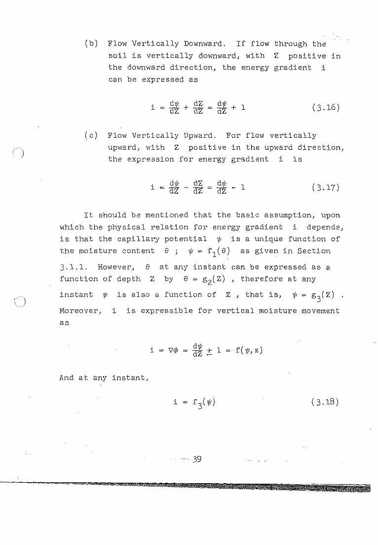
(b) Flow Vertically Downward. If flow through the
soil is vertically downward, with Z positive in
the downward direction, the energy gradient i
can be expressed as
d~1 dZ d'" i = dZ + dZ = ~ + 1 (3.16 )
(c) Flow Vertically llpward. For flow vertically
upward, with Z positive in the upward direction,
the expression for energy gradient i is
(3.17)
It should be mentioned that the basic assumption, upon
which the physical relation for energy gradient i depends,
is that the capillary potential ~I is a unique function of
the moisture content e w = fl(e) as given in Section
3.1.1. However, e at any instant can be expressed as a
function of depth Z by e = g2(Z) , therefore at any
instant 1/1 is also a function of Z, that is, 1/1 = g3(Z)
Moreover, i is expressible for vertical moisture movement
as
i = 'Yep = d1{J + 1 dZ - = f(1/J,z)
And at any instant,
i = f 3(7f!) (3.18)
.~ .. 39

i )
Philip gave a sequence of computed total potential ¢ profiles for the example of infiltration into Yolo light clay
as shown in Figure 3.9. The curves showing the relation
between the total potential ¢ and depth Z are smooth
curves indicating that the total potential ¢ is a
continuous function of the depth Z. By applying those
functions above, therefore, the capillary potential ~ is
a un:i:que function of moisture content e.
o'~-----.--------r-------~------.-------~
I \ I
10 \ , , \ \ , \
20 \ , S I 0 I
" ,
N , \
..c: 30 \-E-
-I-' ' \I P- I OJ
,0 ~
, , 40
, \ , \ I \ \ I
50 \
0 50 100 150 200 250
Total potential ¢ = ~ + Z , cm
Figure 3.9 Computed Profiles of Total Potential ¢
During Infiltration Into Yolo Light
Clay
The nQ~bers on each profile represent
the time in seconds at which the profile
is realized (After Philip 1957d)
40

)
0
20
E !fO (J
" 60 N
l .c +-' So P, ill P I 100
r 120 0 100 200 300 400 500 600
Soi.1 1·1oisturt; Tension '/1, crn
Figure 3.10 Soil Moisture Tension .', , versus
DEp~i1 Z Cur've for Yolo Light Clay
Iii = g.,( Z) (Aft.er Moore 1939) .J
Figure 3.10 shows the soil moisture tension ~ ver'sus
~epth Z curve at Eteady state conditions for Yolo light
clay, ~ - g3(Z) (data ta]cen directly from Moorets paper
1939). In Figure 3.11 the corresponding energy gradient i
versus Z curve is shown. This curve is developed by
evaluating the capillary potential gradients
41

)
desired points in the soil column by drawing tangents to ttle
1/1 = g~(Z) curve (Figure 3.10) and determining ttleir slope. J
1'he energy gradient i is ttlen determined by adding 1.0 to
the aforementioned slope of Figure 3.10.
0
20
S <:)
40 ,
N
..r::: 60 -I-' P. ill P 80
100
120 o
~ 10 20 30 40
Energy Gradient
~
50 60 70
i=0i'.+l dZ
So
Figure 3.11 Ttle Corresponding Energy Gradient i
in an Infiltration Situation for
Yolo Light Clay

)
3.2 NATURAL SOIL CHARACTERISTICS IN UNSTEADY UNSATURATED
FLOW PHENOMENA
In the discussion of unsteady unsaturated flow in
Section 3.1, it was assumed that the energy concept of soil
moisture can be advantageously applied to a wide variety of
soil moisture problems. This is true providing capillary
tension is a function only of the soil water content.
However, this is an idealized approach. The natural charac
teristics of a soil mass in unsteady unsaturated flow are not
a function of soil moisture content alone, but are influenced
by the physical behavior of the texture, structure and
constituents of the soil. Biological and chemical factors
also affect the soil structure. Some of th~ effects are
discussed in the following sections.
3.2.1 THE EFFECTS OF SWELLING AND SHRINKAGE ON THE
STRUCTURE OF SOILS
It is obvious that the swelling and shrinkage of soil
colloids are rather complicated physical phenomena. A soil
) swells when it takes up a liquid as its volume is enlarged
and its cohesion is diminished. The drying of the soil
colloids causes a shrinkage of the soil mass and a cementa
tion of clay particles. The liquid used in swelling may
consist of:
(a) Polar liquids bound at the surface of a solid body
thereby increasing its active volume.
(b) Liquids associated with the solid body as a solid
solution.
(c) Polar liquids reacting with solids to form a
complex compound.
43
j . :1 n
;.; ~
)
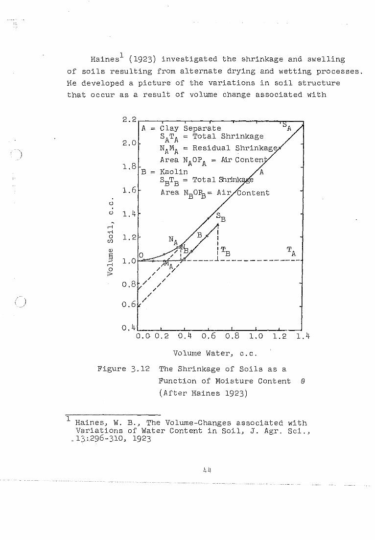
Haines l (1923) investigated the shrinkage and swelling
of soils resulting from alternate drying and wetting processes.
He developed a picture of the variations in soil structure
that occur as a result of volume change associated with
CJ
CJ
" rl .r! 0
CJJ
Gl S ;3 rl 0 :>
2.2
2.0
1.8
1.6
1.4
1.2
1.0
A =
B =
Clay SATA
NAMA Area
separate = Total Shrinkage
= Residual Shrinkage
NAOPA = .Air Conten
Kaolin A SBTB = Total Shr.ink e
Area NBOPB = Air Content
SB
0: 0 ITB TA !-""==i>-_r-;=-----J.-- -- - - --------
0.4~ __ ~ __ ~~~~--~--~--~--~ 0.0 0.2 0.4 0.6 0.8 1.0 1.2 1.4
Volume Water, c.c.
Figure 3.12 The Shrinkage of Soils as a
Function of MOisture Content B
(After Haines 1923)
1 Haines, W. B., The Volume-Changes associated with Variations of Water Content in Soil, J. Agr. Sci.,
_13:296-310, 1923
44

)
varying moisture content. When the volume of soil is
plotted as a function of the volume of water removed, several
significant facts concerning shrinkage become obvious. A
few important curves from his original data are shown in
Figures 3.12 and 3.13. Curve A represents a clay separate
contaj.ning 90.':;% clay, curve B is for kaolin containing ':;2.8,%
clay, and curve D represents a clay subsoil that has been
alternately dried and rewetted.
1.4
<.) 1.3 Clay Subsoil 1. Drying
<.) 2. Rewetted
" 1.2 3. Redried rl 'r! 0
t:I]
OJ 1.1
S rl -0 1.0 :>
0.9 0.0 0.1 0.2 0.3 o. 0.5 0.6
Volume Water, c.c.
Figure 3.13 The Alternate Drying and Wetting
Curves for a Typical Subsoil
(After ,Haines 1923)

In Figure 3.12 it is noted that, as the thoroughly
puddled samples are dried, the decrease in the volume of the
soil is equal to the volume of the water lost. All the
curves are parallel in the wet region and have a slope of l.
As drying progresses, there is a distinct break (points NA
and NB
) in the curve, and the change in soil volume becomes
much less than the volume of water removed. This break
signifies the point at which air enters the soil. Haines has
suggested that this portion of the curve be called II res idual
shrinkage" as distinguished from the total shrinkage that
takes place from complete saturation to dryness. If the
straight portion of the curve is extrapolated to intersect
the vel'tical axis, then the values of OPA and OPB will
represent the volume of the pore space that is occupied by
air in dried soils.
In Figure 3.13 it is observed that the volume of the
reVJetted soil is greater than that of the original. This
increase in volume is permanent after complete drying and is
undoubtedlY,due to the entrance of air into the soil mass,
the air then becoming occluded in the pore spaces. It is
apparei,t that alternate wetting and drying produce
aggregation as a result of unequal strains and stresses that
are set up by shrinkage and swelling processes, together
with the disruptive action of air entrapped in the pores on
wetting. Drying causes a cementation of the clay particles
as the soil mass shrinlcs. Air enters into the pores during
drying. The rapid intake of water during wetting is
responsible for unequal swelling as well as the compression
of the occluded air. Because of these effects there is a
\'ariation in soil structure as moisture content changes. This
val"iation in soil structure alters the permeability of the
soil. The effect is quite pronounced with clayey soils but
practically negligible in the case of sands.
ll6

3.2.2 NON-HOMOGENEITY IN THE SOIL STRUCTURE
Soil structure is defined as the arrangement of soil
particles into certain patterns. The type of arrangement
varies with the amount and nature of the aggregates. Between
the particles in any soil is the pore space. These pores
may be 8mall or large, continuous or discontinuous, depending
upon the type and arrangement of the particles. Therefore
the differences in soil structure will be expressed by:
(a) The structural patte:-n of the various horizons
of the soil profile.
(b) The extent of aggregation.
(0) The amount and nature of the pore space.
From the viewpoint of the permeabi 11 ty of a soil one is
concerned with the shape, size, and distribution of the pore
space. The total porosity of soil is defined as that
percentage of the soil volume which is not occupied by solid
particles. It may be divided into non-capillary and
capillary poroeities. The non-capillary porosity is that
due to the large pores which will not hold water tightly by
capillarity; they are commonly filled with air and are
responsib Ie for the air capacity of' the soil. Capi llary
porosity is attriolJ.table to the small pores that hold water
by capillarity. They are responsible for the water capacity
of soils. A schematic diagram of soil porosity is shown in
Figure 3.1~. It is seen t.hat the Marshall silt loam has
uniform capillary and non-capillary porosities throughout
the entire profile, while in the Shelby loam, the maximum
porosity occurs in the upper 12 inches, and the most
impermeable layer occurs at about 22 to 26 inches below
surface. Because of the difference in distribution of soil
porosity there is a variation of permeability in the Shelby
loam soil column.
47

Non-Capillary Pores
Non-Capillary Pores
Soil Volume
Capillary Pores
Soil Volume
Capillary Pores
o r;:-+-..,.-..;:-r-I-r...,n.71 6
12
18 24 30 36 420~~20~4~0~6~0~8~0~100
per cent of Total Volume
Marshall Silt Loam
o M~"",-,-t,-"""7':f-:n 6
12
18 24 30 36 42
0 20 40 60 80 100
per cent of Total Volume
Shelby Loam
Figure 3.14 Pore-cSpace Relationships in Marshall
Silt Loam and Shelby Loam (After
Baver, 1932)
One of the basic assumptions that is usually made in
the theory of flow of fluids through porous media is that
the medium is homogeneous. This means that the soil medium
has the same permeability at all points. It is often further
assumed that the medium is either isotropic or anisotropic
as regards soil permeability to water under the conditions
of full saturation. If at any point in a soil column the
permeability is the same in every direction, the soil is
said to be isotropic; if it is not the same in eveI'y
direction, the soil is ani sotropic. Because soil structure
is rarely, if ever, truly homogeneous or isotropic, this
presents a problem which must be considered in applying
permeability concepts to the flow problem. If a non
homogeneous soil column is encountered in an unsteady
unsatuI'ated -flow problem, the determination of moisture flow
48

)
will involve a statistical problem of sampling in addition
to the effects of variation of moisture content on
permeability.
3.2.3 BACTERIAL AND BIOLOGICAL INFLUENCES ON SOIL STRUCTURE
There are many puzzling questions associated with the
"?f'fect of' organic matter upon soil structure. l~artin and
Waksmanl (19~O) observed that the growth of' micro-organisms
led to a binding together of soil particles and, consequently,
an increase in soil aggregation. The more readily the
complex organic materials decomposed, the greater was the
effect upon aggregation" The extent of aggregation was found
to be dependent upon the nature of the micro-organisms, the
amount of growth produced, and the nature of the substrate.
Soil fauna are most abundant where there is ample
vegetative cover. This is particularly true in dense sods
and good forest covers. The soil under a thick forest litter
is permeated with the channels of earthworms and other biotic
life. These channels make the soil rapidly permeable to
water. Removal of the litter by burning or pasturing
destroys the basic condition that favors the development of
an abundant soil flora. TJ1e permeability of the soil
disappears along with the decreasing biotiC activity. This
fact was confirmed by the data of Auten2 (1934), who found
that the rate of absorption of water by soils in burned
1
2
Martin, J. P., and Haksman, S. A., Influence of micro-organisms. in soil aggregation and e'rosion, Soil Sci., 50; 29-47.. 191fO
Auten, J. T., The effect of forest burning and pasturing in the Ozarks on the water absorption of forest SOils. U.S. Dept. Agr. Forest Service, Central states Forest Exp, sta. Note 16, 1931f
49

woods was only about 20% as fast as in natural undisturbed
oak woods.
The permeability of a given soil in a given area is
subject to change depending on the bacterial and biological
activity. Often these activities are a functicin of termpera
ture and moisture content. Hence most soils exhibit seasonal
changes in permeability.
3.2.4 EFFECT OF CHEMICAL CHARACTERISTICS OF THE WATER
There are many factors that affect the movement of
vlater through soils and cause difficulty in making
permeability determinations in both the laboratory and field.
Most soils may be classed as unstable materials whose size
and arrangement of pores change as a result of the passage
of water through the media.
It is common knowledge that the quality of the water
which percolates through the soil has a marked effect upon
the permeability of the soil. The electrolyte concentra
tion influences the permeability of most soils. It has been
observed -by a number of investigators that the permeability
of soils decreases with time after water is applied.
Bodman l (1938) indicated that the "Explanation of the great
decreases in saturated water permeability of all of the
soils examined seems to lie in the early removal of
electrolytes and subsequent gradual dispersion and rearrange
ment of the clay particles so that the conducting pores are
l"educed in size more or less permanently."
1 Bodman, G. B., The variability of the permeability constant at low hydraulic gradients during saturated water flow in soils, Soil Sci. Soc. Amer. Proc. 2:45-53, 1938
50

Fireman2 (1941,) has stated that if the amount of
sodium in the irrigation water is high compared with the
8JJlOunt of other salt contents (calcium plus magnesium), the
soil will not take water readily. The soil particles will
disperse and tighten up the soil reducing the size of the
pore spaces, therefore the soil i'iill become sticky and
relatively impermeable. -,
Quirk and Schofield.) (1955) presented quantitative data
showing the decrease in permeability as a function of the
electrolyte concentration of the water for soils having
various exchangeable sodium levels. They also presented a
relationship between exchangeable sodium percentage and
electrolyte concentration for which permeability was either
stable or decreasing. Figure 3.15 shows varying the
concentration of irrigation water in order to maintain a
stable permeability condition.
2 Fireman, M., Permeability measurements on disturbed soil samples, Soil Sci. 58:337-353, 1944
3 Quirk, J. P. and Schofield, R. !C., The effect of electrolyte concentration on soil permeability, Jour. Soil Sci. 6;163-178, 1955
51

I,
il i-
ii :; i: i. I' , , I: j,; . ,-,,, I,: . i: Ii'
I:. ~ ; '"
,,,,. "ii" -"I
:'"
';1
S .,-l 'd 0 60 Ul
Cll M so .g Cll bD >=: 40 cO ..c: CJ ~ 30
1'<1 QJ
bD cO
20 +-'
>=: 10 Cll CJ H Cll 0 P-<
0
Decreasing permeability
----
- Stable permeability
5 10 15 20 25 30
g :g M o Ul
s UJ
& 'd QJ
+-' cO H ;:l +-' cO Ul
3S
Electrolyte Concentration (milliequivalent per liter)
Figure 3.15 The Electrolyte Concentration of
Irrigation Water Required to maintain
a Stable Soil Permeability for Varying
Degrees of Exchangeable Sodium
Saturation
(After Quirk and Schofield 1955)
52

If. A]I)ALY'rrCAL APPROACH TO THE SOLUTION OF
UNSTEADY UNSATURA'l'ED FLo\v PROBLE~1S IN
SOILS--WRITER'S ANALYTICAL WORK
--STRIP METHOD
4: 1 'I'HE NATURE OF UNSTEADY UNSATURA'l'ED FLOW IN SOILS
The nature of uniitEady unsaturated 'flow in soils can
best be seen by examining a particular example of such flow.
Take the case of infiltration, Figure 4.1. At some time tl
after the onset of infiltration the mOisture distribution in
the soil will be approximately as shown in Figure 4.1a and
i+'lb. A short time (6t) later the moisture distribution
will be as shown in Figure " 1 Lr • ...L C .
It should be mentioned here that 9 i , the inactive
moisture content (Sec. 3.1.2) i.s defined as that mOisture
which does not contribute to the flow through the soil, and
90
' the threshold moisture content is the lowest moisture
content at which a soil exhi bi t s permeabi Ii ty. Therefore
at any given level in the soil, where the wetting front has
preceded this level, the moving moisture content should be
considered as the difference between total moisture content
9 and inactive moisture content 9 i However, the value
of 9 i is generally unknown and in most instances it may
be assLUned approximately equal to 90 , When applying the
continuity principle only the net excess of flow of water
into and out of any volwne element is considered. Therefore
the effective moisture content 9' is equal to total
moisture content 9 less the inactive moisture content 9i
.
Since it is assumed that 8i = 80 .' the effective moisture
content 8' = 8 - B_ u
53

z z
(a-B)
( a) ( c)
t = tl t = t + lit
Figure 4.1 MOisture Distribution During Infiltration
(Assumption a ~a a ~a ) Inactive- Threshold' i- 0
In Figure 4.2 is depicted an infiltration situation.
Here, infiltration is used for purpose of example only.
Capillary rise or any other unsteady unsaturated flow situa
tion could have been used .just as well. The moisture profile
is divided into a number of horizontal strips. Under initial
conditions the moisture distribution is as indicated in
Figure 4.2a. The corresponding permeabilities, soil moisture
tensions and energ\' gradi ent s are shown in Figures 4. 2b,
4.2c, and 4.2drespectively.
S4

z
!"'- (B2
-B O)
f.!--- (B3-~ L-----"'
(a) Moisture Distribution
z
(c) Soil MOisture Tension
(Capillary Head)
Figure 4.2 Infiltration
55
Z
Z
K'J-----I c:
(b) Permeability
(d) Energy Gradient
i = ~ + 1 dZ

4.2. DARCY'S LAlf AND CONTINUITY PRINCIPLE APPLIED TO
UNSTEADY UNSATURATED FLOW
In the case of an unsaturated medium the question
arises as to whether or not Darcy's law is applicable. In
an unsaturated soil a portion of the void space is filled
with air. Since air inclusions effectively prevent water
flow through themselves, they maybe replaced by a solid
phase and the result would be a saturated medium. It may be
seen then that the presence of air in the pore space has the
effect of reducing the volume of the medium available for
flow of water and does not itself invalidate Darcy's law.
Childs and George l (1950) working with unsaturated sands
found that at a given moisture content, Darcy's law was
valid.
It may be expected that there is a limitation to the
application of Darcy's law in unsteady flow. However, for
most flow problems in soils, the gross velocity is very low.
Each element of water moving through a porous medium follows
a continuous.ly curvilinear path at a continuously varying
speed and with a varying acceleration. The magnitude of the
!) gross acceleration is rather small compared to the velocity,
therefore it seems reasonable to assume that Darcy's law is
applicable to unsteady flow.
Darcy's law is not sufficient to determine a given flow
problem. In addition, the flow of water must satisfy the
equation of continuity. This may be expressed for the
writer's purpose as: "the net excess of flow of water into
and out of any volt@e element is equal to the change in
storage within that VOlume element". This means that the
water is treated as a continuouE' medium and its motion is
governed by Darcy's law.
1 Chi Ids, E. C. and George, N. C., Permeability of porous materials, Proc. Roy. Soc. (London), 210A: 392-399, 1950
56

( )
)
4.3 DERIVATION OF DIFFERENTIAL EQUATI0N OF INFILTRATION BY
CONCEPT OF FIXED SECTION
It is the purpose of this section to derive the
differential equation of infiltration from the viewpoint of
a fixed section, and to interpret tll.e relation between the
matll.ematical differential equation and tll.e grapll.ical
numerical procedure.
Tll.e equation of infiltration as expressed by Philip was
de clt =
wll.ere D = K~ cle
Therefore,
Cle dt =
=
=
This means that,
(de) dt
" (D de) ClK 0 ( 4.1) dz - dz dz
Cl
(K * de dK dz dz) -dz
, (K Clw) ClK 0
clz dz' - dZ
Cl (K (~ 1» dz -
(4,2) z = constant constant
If two sections that are fixed in space are taken,
Figure 4.3, then at time t = tl and t = tl + dt , the
corrsponding moisture distribution, permeability K, and
energy gradient i are as indicated in Figures 4.3a and
57
1 1
I , I,
.I
" I ,I ,,' j q:

)
. . . ~
)
4.3b, since K at any time t is also a function of z as
is the i at the time t .
T dz
T dz
K
(K+ ~ dZ)
(a)t=tl
j (K+ ~ dt)
o( K+ ~K dZ) (K+ ~ dz)+ ~t dt
(0) t = tl + dt
i
(il~; dZ)
(il ~; dt)
d(il~~dZ) (il~; dz)+ d~ dt
Figure 4.3 Schematic Diagram of Moisture Profile
for the Fixed Section During
Infiltration
58

Applying Darcy's law and the continuity principle to a
fixed section, one can write:
(Volume of Inflow during dt)
Ki + I = A (
. dK ) ( lK + dE" dt i +
2
di "t) df Q ) dt
where A is the gross cross-sectional area through which
the flow ib occuring.
) Neglecting higher order terms,
! )
K %~ dt + i * dt I ':;; A (Ki + -=-=--~2--=":'c---) dt ( 4 .3)
(Volume of Outflow during de)
O=A
Again, neglecting the higher order tenns and combining the
remaining terms one gets,
(4.4)
Subtracting Eq. (4.3) from Eq. (4.4)
o - I = A (K~dZ + i~~dZ) dt ( 4.5)
Since (Volume in) minus (Volume out) l"Iill be equal to 6S,
the change in storage duriEg dt
59
---------------------------------====.= .... ~--~

68 = AciBdz (4.6)
Therefore equating Eq. (4.6) to Eq. (4.5), gives
AdBdz = A (K ~dZ + i ~dZ) dt (4.7)
Dividing both sides by Adzdt ,
(~. 8)
that is,
dB = d(Ki) dt dz (4.9)
same as Eq. (4.2).
From the foregoing derivation one may state that the
differential equation of infiltration is the expression at
an instant as regard to a fixed section, and using the
difference (denoted by 6) instead by differential, then the
geometrical interpretation of Eq. (4.9) can be explained as:
the slope of the product of Ki at a particular section is
equal to the rate of change of moisture content at that
section at the particular instant of time under consideration.
The geometric interpretation is shown schematically in
Figure 4.4.
60

1---... (8 - 80 ) -,--
z
f---......... Ki
z
Figure 4.~· The Geometrical Interpretation of
Infiltration Equation
M = 6(Ki) 6t 6z
61
¢ft.;
6z

'.
'. \ !
t
" .',
'.
.!.
" i ,
4.4 ANALYSIS BY STRIP METHOD USING CONCEPT OF MOVING SECTIONS
HAVING FIXED MOISTURE CONTENTS
An infiltration situation is depicted in Figure 4.5.
The moisture profile is divided into a number of horizontal
strips, a straight line connecting the extremities of
adjoining strips. The dashed line shows the moisture profile after time interval (f',t)
8SAT
f zl
+- 81 Ml 8N
_l
+ Z 2 zN
~ 82 +- 8N
i 3 8
3 f', Z2 zN+l 8 • ,
~ ~ ~~-IM z4 *
-~-~\8 3
f',z 3
4 llz4
( a)
Figure 4.5 Moisture Distribution During
Infiltration
62
(b)
a (f',8N_l
I
!}MN
~ ' f',zN

In this approach it is assumed that the moisture
content 8 of a section in the soil is increasing by an
amount (68) during the time interval (6t) and that the
posi tion of the original moi.sture content 8 moves a
distance (6z) durinc that time interval. On this basis it
is possible to derermine the net movement (6~) of the
position of' any particular moieture content during the time
interval (6t) ,
Referring to
of the slopes of
Figure 4.5b and using the weighted average
lines ab and bc to express the slope
68N
6zN at point b one may I'lri t e :
( 4 . 10)
where 68N
is the grcl'ith of the moisture content during the
time int erval (6t) at the Nth level.
More specifically,
(4.11)
8 1 - 82 8
2 - 8~
68 2 ( z )( z3) + ( z .J)(z2)
2 3 6z2
= Zn + ~~ co .J
(4.12)
etc.
63
ali""'!! W2£1-U AFila MIE

, , ,. to. , I .... i ) , .'
" , j' .. n.
L
.o.
r
'. ,
From the differential equation of infiltration, and
using the difference (denoted by 6) instead by differential,
one may write Eq. (4.2) in the following fashion:
(4.13)
or
(4.14)
therefore, according to Figure 4.5 and using the weighted
average of the product Ki, this can be written as
and
KSATiO - Kli l ( 21 )(20)
~
68 1 = 21 +
Kli l - K~i2 ( , c:: )(Z.,) +
"'2 .J 68 2 =
22 +
etc.
Kli l - K i + ( ~ 2 2)(2
1)
~2
22
K2i2 - K i ( .. 3 3)(z2)
~3
z., .J
(6t )
(6t)
(6t )
(4.15)
(4.16)
(4.17)
substituting Eq. (4.16) into Eq. (4.11) and Eq. (4.17)
into Eq. (4.12) etc., one can solve for 6z 1 , 6z2 , etc.
64

K i - K i K i - K i ( SAT 0 1 l)(z ) + ( 1 1 2 2)(z )
zl 2 z2 1 6z1 = -e"S-A-T--=-;;-e ----'e,---"e--'''------- (6t)
(-=:":=--Z_~1)(Z2) + (\ 2)(Zl) 1 2
and
Substituting Eq. (4.15) into Eq. (4.10), the general
expression will be
( ~_liN_1 - ~iN)( ) + (~iN - ~+liN+1)(z )
(1j.1S)
(4.19)
zN zN+1 zN+1 N /',zN = ---*---,,---------r;---';i-'-'-'------- (/',t) e BN e - B
( N -1 _ ) ( ) + (N N+ 1) (z ) " zN+1 Z N ~N N+1
(4.20)
If the strips are of equal height, that is
etc. (4.21)
or
( 4. 22)
Equations (4. lS), (4.19) and (4.20 ) become :
65

f:: :! , "
i
• • , ! ; , , , ,.
--,
"
i [-, ,. !,: I,
... I'; ,', ,
1i.
i , '-,. :' .
. "-'0
)
)
f'bnam
(KSATiO - K i ) L1z 1 = (8SAT
2 2 (L1t) 8 2 )
L1z 2 = (Kli l - K3i 3)
(L1t) (8 1 - 83
)
etc.
And the general equation for L1z N
is
L1z = N
( 4.24 )
(L1t) ( 4.25)
However, in most instances the height of the strips
need not be equally spaced, thus using Eq. (4.20) one can
simplify as following:
( 4.26)
where L1zN is the movement ::>f the Nth section moisture
content during time interval (L1t) , zN' 8N , ~ and
iN are the height of the strip, moisture content,
permeability and energy gradient of the soil at Nth level
as defined before.
The procedure above can be followed through successive
strips until they have all been considered, thus the movement
of each section's moisture content will represent the
progress of the moving front during the time interval (L1t)
This then gives the ]Jew moisture profi1e at the end of the
first time interval. By repeating the entire process again,

-
the moisture profile at the end of sucGessive time
intervals can be ascertained.

"
, "
'. ,.
,
'P'iii!'8&errmm RF7Srmwr:m 11 wm twrrm rnnmmnt'13'iW"f' - , '5 ! iirl 7 FE if WXS~
5.1
5. THE GENERAL OUTLINE OF THE
NUMERICAL PROCEDURE
THE BASIC DATA FOR ILLUSTRATIVE EXAMPLE
In order to apply the strip method to any flow
situation, one must have knowledge of the physical and
hydraulic characteristics of the soil. That is; the general
nature of soil moisture tension ~ = fl(e) , permeability as
a function of moisture content K = f 2 (e) , and the physical
relation for the energy gradient i = f3(~) as outlined in
Chapter 3 must be known. Also, the initial moisture
distribution must be known or assumed.
For illustration, the example presented here is for
infiltration. In this example water is infiltrating into
Yolo light clay. The data are taken directly from Moore's
paper (1939 ) as shown in Table 5.l. These data are the
wetting soil moisture tension ~, and permeability K as
functions of mOisture content e for that soil. They are
shown in Figures 5.1 and 5.2 respectively. The initial
moisture distribution is chosen from Philip profiles at
a
time t = 3.5xl05 seconds. This profile is divided into 11
strips. The value.s employed in the computations are given
in Table 5.2. Starting with these data the strip method is
applied through a step-by-step procedure.
68

-j
-)
i&ii4lJ:U+ ;4
Table 5.1 Wetting Soil Moisture Tension 1/1 and Permeability
K as Functions of Moisture Content e (Apparent
specific gravity of Yolo light clay = 1.32)
Moisture Content e Soil Moisture Permeability
Per cent Tension 1/1 Kx106
by Weight by Volume em em/sec
37.5 0.4-950 0 12.3
37 0.4-884- 8 8.60
36 0.4-752 16 6.15
35 0.4-620 22 4-.4-0
34- 0.4-4-88 27 3.30
33 0.4-356 32 2.56
32 0.4-224- 37 1.91
31 0.4-092 4-4- 1.4-8
30 0.3960 50 1.21
29 0.3828 58 1.06
28 0.3696 67 0.97
27 0.3564- 76 0.88
26 0.34-32 86 0.795
25 0.3300 108 0.398
24- 0.3168 14-0 0.215
23 0.3036 172 0.133
22 0.2904- 224- 0.091
21 0.2772 278 0.064-
20 0.264-0 366 . 0.04-1
19 0.2508 4-4-0 0.022
18 0.2376 592 0.012
69
4t&'f FM ;;4. db g Am;;;- Ii

(;1
! f I;'
Ii; " I:; ,<'
" II!
) 1;'( "I ", I';. l~~
'" I-j.
", f" .,' ~:
'r', :.! , .. '" n .;
"
' .
. . , , " ..
S ()
'i>-
~ 0 ·rl 1ll ~ OJ
8
OJ H ::J +' 1ll ·rl 0 ~
rl ·rl 0 Cfl
600
500
400
300
200
100
O~&-______ -L ______ ~ ________ -J __________ ~ __ ~~ __ ~
20 25 30 35 40
MOisture Content e (by Weight)
Figure 5.1 Curve of Soil Moisture Tension '"
versus Moisture Content e for Yolo
Light Clay (After Moore 1939)
70

1
0 1 QJ Ul
"-S 0
'-0 0 rl 8 Q p.,
-l-' ·rl rl ·rl .0 6 ctI QJ
S H QJ
Il;
4
2
•
"
20
Moisture Content B (by Weight)
Figure 5.2 Curve of Permeability K versus
Moisture Content
Clay (After Moore
71
B for Yolo Light
1939)
}[
.'Ii
, , --.-
J~ ~ i ;' i

(/ ! I
, .-" r,; '" 1':: , .... r'!, ,----", . } , . ... ,., 'l' \111
t~
" .,. ,~! 0'1-'
;.i:; .. ,. H,
~~ )~r
I.: ., \,
: ,~,
. iT '>lr
'i . , ; ',~;
" ..
Table 5.2 Values of Soil Moisture Tension ~ and
Permeability K used to compute Infiltration
Into Yolo Light Clay
Moisture Content e Soil Permeability Moisture
Moisture Kxl06 Distribution
Tension Z em
by Weight by Volume ~ em em/sec Philip Profile
at t=3.5xl05
seconds
37.5 0.49500 0 12.300 0.00
35.8 0.47256 18.0 6.150 25.80
34.1 0.45012 26.0 3.150 30.70
32.4 0.42768 35.0 2.190 32.80
30.6 0.40392 46.0 1.570 34.80
28.8 0.38016 59.0 1.100 36.60
27.0 0.35640 76.0 0.780 38 .~O
25.2 0.33264 105.0 0.~35 40.90
23.4 0:30888 158.0 0.175 43.50
21.6 0.28512 245.0 0.085 45.60
19.8 0.26136 375.0 0.049 48.00
18.0 0.23760 592.0 0.012 54.90
..
72

5.2 THE NUMERICAL EXAMPLE OF HAND CALCULATIONS
Table 5.3 shows the hand calculations for the first
two time intervals. A time interval of 4 bot = 1. 5xlO
seconds is used.
eViden6ed in this
A column by column explanation is self
table. Footnotes indicate some of the
details of the computations. These required about six hours
of work, approximately three hours for each time interval.
73

" ,
'/ ," ,I,
I,
, '~ "I, ~ ,I, d' ,1,-
:~t , '" I,
'" ", ,
\~~ i ",
:;t !~~
u,;;
!.i. " '~~ !
"n
" I'
I ~:,
H'
~~
;~! '" ..
Table 5.3 Sample Computations of Infiltration Into Yolo
Light Clay by Strip Method
(1) ( 2) ( 3) ( 4 ) ( 5) ( 6)
Section eN eN eN
_1 - eN "'N "'N - "'N -1
wt Vol Vol em = 6",N em
1 37·5 0.49500 0.0
2 35.8 0.47256 0.02244 18.0 18.0
3 34.1 0.45012 0.02244 26.0 8.0
4 32.4 0.42768 0.02244 35.0 9.0
5 30.6 0.40392 0.02376 46.0 11.0
6 28.8 0.38016 0.02376 59.0 13.0
7 27.0 0.35640 0.02376 76.0 17. 0
8 25.2 0.33264 0.02376 105.0 29.0
9 23.4 0.30888 0.02376 158.0 53.0 10 21.6 0.28512 0.02376 245.0 87.0
11 19.8 0.26136 0.02376 375.0 130.0
12 18.0 0.23760 0.02376 592.0 217.0
74

Table 5.3 (Continued)
( 7) (8) ( 9) ( 10) (ll)(a) ,
K ZN 'V1/IN Wt. ('V1/I)N ,
ZN 1: :
106 em = ZN - ZN_l = ( 61/1) 6Z N
em/sec = 6ZN ::
em .,;;~ ~!! ~!: .,q , -',<,j -,
12.300 0.00 ,;ti h'U "' 6.150 25.80 2S.80 0.6977 1.4831t -,;
::Ii ,;i;
1. 6326 3.4898 3:1
3.150 30.70 Jt .90 ~~!
~I
2.190 32.80 2.10 4.2857 4.9077 --:1 ~ !
:~j
1. 570 34.80 2.00 5.5000 6.4064 ,;! ,-:: ";:,
1.100 36.60 1.80 7.2222 8.3333 ," :ii
0.780 38.40 1.80 9.4444 10.3467 [1
0.435 40.90 2.50 1l.6000 15.9062 ~
0.175 43.50 2.60 20.3846 32.0260 !ti .. _.
0.085 45.60 2.10 41. 4286 47.3730 ,,,.
ii 0.049 48.00 2.40 54.1667 48.3041 1~
49.2352(b) ~
0.012 54.90 6.90 31. 4493 Ii !~ ;~ " -, ~ i~ ;~ H
.!:
Notes: " il
('V1/IN) (zN+l) + ('V1/IN+l) (zN) ( a) wt. ('V1/I)N = ( zN zN+1 J +
(b) wt . ('11/1) 12 = 2(wt. ('V1J)1l) - ( wt . ('11/1) 10)
75
-41;;:U4i£ZiJw= ,_' _ _ _2!luttJWZ.iWtiiiWi1i£J.illZ\¥Q!ii ,e*~~?5j§P $4liUi!lM;Z;;hi--*M~c:: .. ;;;g~

Table 5.3 (Continued)
( 12) ( 13) (14 ) (15) . ( 16)
d~ zN+zN+l iN ~~N EN_liN _l-ENiN ( ZN)2
" !h 106 106 2 ""- em = wt.(V1J!)N+l
em
i ~; '~~ . em/sec em/sec • i~
". Mf!( I!l:
I" 11~ . . ~~ 30.70 2.4834 15.2729 665.64 " ."~
1'" 7. 00 4.4898 14.1429 1.1300 24.01 tJ:, i:
.~- 4.10 4.41
'.l~ 5.9077 12.9379 1. 2050 ,j~ ,. ';~ 3.80 7.4064 11.6280 1.3099 4.00 It~
I} 3.60 9.3333 10.2666 1. 3614 3.24
" 4.30 11.3467 8.8504 1. 4162 3.24 ·~L .
. ~~ 5.10 16.9062 7.3541 1. 4963 6.25 Ii,
" 4.70 33.0260 5.7796 1. 5745 6.76 .. . , 4.50 48.3730 4.1117 1.6679 4.41 ;
., ':' 9.30 49.3041 2.4159 1.6958 5.76 '" " "i! 50.2352 0.6028 1.8131 47·61 <, ", !-.

)
Table 5.3 (Continued)
( 17) 2
(lIKi)N( zN+l)
+(lIKi)N+l(zN)2
106
cm3/sec
33.9154 10.5967 9.6897 8.9994
13.6993 19.9556 18.2185 17.0856 91.1805
Notes: ( c) Eq. ( 4.26)
(18)
(MN) ( zN+l) 2
+(6BN+l)(zN)
2 cm
15.4757 0.6377 0.1945 0.1720 0.1540 0.2255 0.3091 0.2654 0.2416 1. 2681
2
where 4 6t = 1.5xl0 seconds
( 19) ( c) ( 20) ( g)
6zN ~'
cm = ZN+6zN
cm
O.OOOO(d) 0.0000
0.7784(e) 26.5784 0.7978 31.4978 0.8172 33.6172 0.8450 35 .. 6450 0.8766 37.4766 0.9113 39.3113 0.9684 41.8684 1.0297 44.5297 1.0608 46.6608 1.0785 49.0785
1.1446(f) 56.0446
(d) lIz1 = 0.0 , there is no growth at 1st section, that is at the surface of the ground.
(e) lIz2 = 2(6z3) - (6z4)
( lit) ( f)
( g) Z I N
is the new mOisture profile at the end of the
first time interval.
77

";
, " : II'
· 1!:r
: I~~. I;';:
, .. ~~, 1'''<,1
, I'~ · r~'. , j;, i ,',) : 1'1"' ~ , I·~ , .. ,,, , Ir. ...
-" :: -q~" "
· :'ll" iU ;, I~.! t- .:~ ::: _I~~
(:-I~~ ~' .• '~1 .
: ·I~".
! ,~;; , '~"
, ,
Table 5.3 (Continued)
( 21) (22)
ZN 1 'V1/IN 1
= ZN 1 -ZN_l 1 !EL = (t;Z')N = ~' , em
26.5784 0.6772 4.9194 1.6262 2.1194 4.2465 2.0278 5.4246 1.8316 7.0976 1.8347 9.,2658 2.5571 11.3410 2.6613 19.9151 2.1311 40.8240 2.4177 53.7701
6.9661, 31.1509
(23) (a) (24) wt . ('11/1 1 ) N zN'+zN+l
,
em
1. 4780 31. 4978 3.4575 7.0388 4.8486 4.1472 6.3036 3.8594 8.1808 3.6663
10.1327 4.3918 15.5424 5.2184 31. 5262 4.7924 46.8892 4.5488 47.9424 9.3838
48.9956(b)
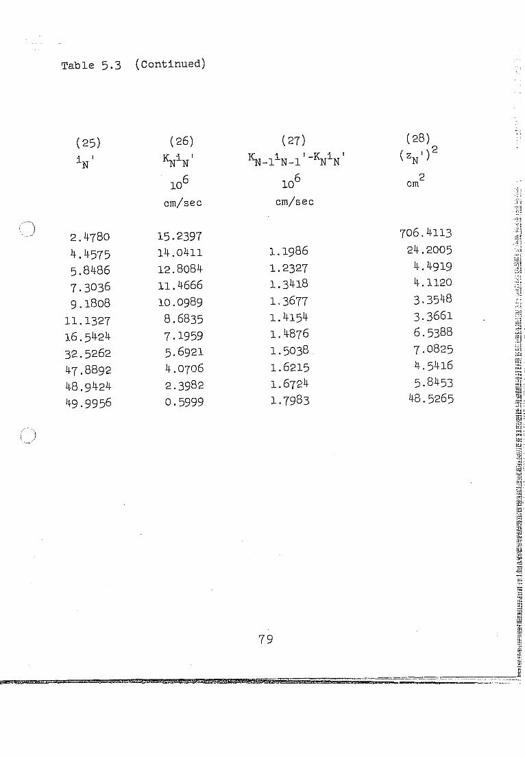
Table 5.3 (Continued)
( 25) ( 26)
iN ,
~iN ,
106
em/sec
2.4-780 15.2397
4-.4-575 14-.04-11
5.84-86 12.8084-
7.3036 11. 4-666
9.1808 10.0989
11.1327 8.6835 16.54-24- 7.1959 32.5262 5.6921
4-7.8892 4-.0706
4-8.94-24- 2.3982
4-9.9956 0.5999
:)
(27)
~-1 i N_1 ' -~iN ,
106
em/sec
1.1986 1.2327 1.34-18 1.3677 1. 4-154-1.4-876 1. 5038. 1.6215 1.6724-1.7983
(28) (zN' ) 2
2 em
706.4-113 24-.2005
4-.4-919 4-.1120 3.354-8 3.3661 6.5388 7.0825 4-.54-16 5.84-53
4-8.5265
'i:
':1 ~ ,
.~ ~ ~~ ,

~; r.:ii ,'i
~-. ', .. ; 1 :~i; ,II,
''1:, - ~,.
; .~::-: ., 1:1
/" "~Ii !. '-:.~~' , ;, ~i! ; 1.- 'i!
L ,~,
~. ,~, ;, ,;'
i r ! I
""
)
)
Table 5.3 (Continued)
( 29)
(Mi')N(zN+l,)2
+( Mi ' )N+l (zN') 2
106 , cm3/sec
35.2159 11.0961 10.1255 9.3522
14.2624 20.3690 18.3139 17.0735 91.6673
(30) (31)(c)
(MN) (zN+l') 2 zN ,
+(MN+l) (zN,)2 em
cm2
O.OOOO(d)
16.3949 0.8045(e)
0.6439 0.8204
0.1990 0.8363 0.1774 0.8561
0.1597 0.8784
0.2353 0.9092 0.3236 0.9442 0.2762 0.9946 0.2468 1.0377
1. 2919 1.0643
1. 1353( f)
so

Table 5.3 (Continued)
Z 11
N
= Z '+6z ' N N
cm
0.0000
27.3829
32.3182
34. ~535 36. ':;.011
38.3550 40.2205 42.8126
45.5243
47.6985 SO .1428
57.1799
Notes:
Repeat Columns
(21)--(32), etc.
( h) Z 11 is the moisture profile at the end of the second N
time interval.
,·l

5.3 A BALGOL PROGRAM THROUGH USE OF THE BURROUGHS 220
DIGITAL COMPUTER
The hand computation procedures are quite lengthy so
that computations have been carried out through use of a
digital computer. The aspects of the BALGOL program for the
infiltration example are shown in Table 5.4.
In programming the strip method, one is able to take
advantage of the procedure calling which is a sub-program
of BALGOL. Thus the time interval can be selected either in
equal or unequal intervals. The writer has -made two runs
using the initial moisture distribution at t = 3.5X10⁵
seconds, one with equal time intervals of lit = 1.0X10⁴
seconds for 65 intervals, the other with unequal time
intervals of lit = 1.5xl04 seconds for the first ten
intervals, then lit = 2.0xl04 seconds for the next ten
intervals and finally lit = 3.0X10⁴ seconds for the last ten
intervals. Moisture distributions at times t equal to
5.0X10⁵ seconds, 7.0xl05 seconds and 10xl05 seconds are
plotted in Figure 5.3. The Philip profiles are also depicted
in the same figure. Their corresponding values are presented
in Table 5.5.
The writer has also selected the second initial
moisture distribution from Philip profiles at t = 10xl05
seconds.·' (The reason for this selection will be discussed
in Section 6.2). Equal time intervals of lit = 5.0X10⁴
seconds for 50 intervals were used. Moisture distributions
at times t equal to l5xl05 seconds, 20xl05 seconds,
25xl05 seconds, 30xl05 seconds and 35xl0 5 seconds are
plotted in Figure 5.4. Also, the Philip profiles are shown
in the same figure. Their numerical values are presented in
82

Table 5.6. The machine time amounted to about 10 seconds
per time interval for each run.. All results computed are
listed orderly in Appendix B.
83
, .c'l

;: i
, ,'I'
"1 " !.,,) :
:: , ;,;1 ,i
. ,
." '
.:'~~ ! -~',.: 1-
"" .,,'" ... _;:,' 'I
'" ~ . ,,~ ':::':i "
", .:
Table 5.4 Example of BALGOL Program for Infiltration Into Yolo Light Clay
$$$ TIME ON 1244 FRIDAY, 11/30/62
*S480 BALGOL 5 MIN. FLORA C. WANG CE DEPT. EXT. 2321 FW1 BURROUGHS ALGEBRAIC COMPILER-STANFORD VERSION 10/20/62
COMMENT APPLICATION OF STRIP METHOD TO INFILTRATION PHENOMENON $
INTEGER N, M, P, Q $
BOOLEAN B $ ARRAY Z(2,12), THETA(12), K(12), PSI(12), GPSI(12),
HZ(12), WPSI(12), 1(12), DELZ(12) $ INPUT DATA(N,Z(l,N),THETA(N),K(N),PSI(N)) $
WRITE($$HED) $ RD.. READ ( $B$DATA) $ IF B $ GO NEXT $ FORMAT HED(B4,*N*,B9,*Z*,B9,*THETA*,B11,*K*,B12,
*PSI*,W3)$ WRITE ( $$OUT1, FORM1) $ OUTPUT OUT1 (N ,Z (1 ,N) ,THETA (N) ,K(N) ,PSI (N)) $
FORMAT FORM1(B3,I3,B3,X10.4,B3,X9.5,B3,F12.5,B3,X7.1, WO) $
GO RD :~
NEXT .. PROCEDURE STRIPMETHOD(DELT,P,Q$Z(,),THETA(), K(),PSI()) ~,
BEGIN
INTEGER N,M,P,Q $
ARRAY GPSI(12) ,HZ(12) ,WPSI(12) ,1(12) ,DELZ(12) FOR M = (P,l,Q) $
BEGIN WRITE($$NEWM,SKIP) $ OUTPUT NEWM(M) :~
FORMAT SKIP(*M = *,Il4,W3) $ FOR N = (2,1,12) $
FW2 FW3 FW4 FW5 FW6
FW7 Fw8 FW9 FW10
FW11 FW12
FW13
FW14
FW15
FW16
FW17 FW18
$ FW19 FW20 FW21 FW22
FW23 FW24
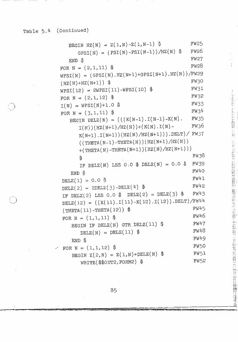
Table 5.4 (Continued)
e.%QIJ4I:;:;UdIAd_
BEGIN HZ(N) = Z(l,N)-Z(l,N-l) $ FW25
GPSI(N) = (PSI(N)-PSI(N-l»!HZ(N):$ FW26
END :ip FW27
FOR N = (2,1,11) I FW28
WPSI(N) = (GPSI(N) .HZ(N+l)+GPSI(N+l) .HZ(N) )/FW29
(HZ(N)+HZ(N+l» I FW30
WPSI(12) = 2WPSI(1l)-WPSI(10) I FW31
FOR N = (2,1,12) $ FW32
I(N) = WPSI(N)+1.0 G FW33
FOR N = (3,1,11) 8 FW34
BEGIN DELZ(N) = (((K(N-l).I(N-l)-K(N). FW35
I(N) )(HZ(N+l)/HZ(N) )+(K(N) .I(N) - FW36
K(N+l) .I(N+l) (HZ(N) /HZ(N+l») .DELT)/ FW37
( (THETA (N -1) -THETA (N) ) (HZ( N+l) /HZ( N) )
+(THETA(N)-THETA(N+l»(HZ(N)/HZ(N+l»)
$ ~38
IF DELZ( N) LSS O. 0 :~ DELZ( N) = 0.0 ·t\ FW39
END $ Fw40
DELZ( 1) = 0.0 !$ Fw41
DELZ( 2) = 2DELZ(:3) -DEL2,( 4) I Fw42
IF DELZ(2) LSS 0.0 $ DELZ(2) = DELZ(3) 11> Fw43
DELZ( 12) = ((K( ll). I( ll) -K( 12) .I( 12» .DELT)/FVJ44
(THETA(11)-THETA(12» I Fw4S
FOR N = (1,1,11) $ Fw46
BEGIN IF DELZ(N) GTR DELZ(ll) $ Fw47
DELZ(N) = DELZ(11) I Fw48
END $ Fw49
FOR N = (1,1,12) $ BEGIN Z(2,N) = Z(l,N)+DELZ(N) $
vJRITE($$OUT2,FORM2) $
85
FW')O
F\1':;l
FW52
~-;. _ . .,.- ... : .
.;., :
'''-, , :T-l . :.:; .
: f. ~
"""' :jl
;;,j.
J

Table 5.4 (Cant inued )
OUTPUT OUT2(N,Z(2,N)) :II> FW53 FORMAT FORM2(B3,I3,B5,Xl0.4,WO) :II> FW54 Z(l,N) = Z(2,N) :II> FW55
END :II> FW56 END $ FW57
RETURN END $ FW58 STRIP METHOD (1. 5**4,1, lQ:~Z ( , ),THETA ( ), K( ), PSI ( ) ) $ FW59
) STRIPMETHOD(2. 0**4,11 ,20$Z( ,) ,THETA ( ) ,K() ,PSI()) $ FW60 STRIPMETHOD(3.0**4,21,30$Z(,),THETA(),K(),PSI()) :Ip FW61 FINISH $ FW62 COMPILED PROGRAM ENDS AT 0791 PROGRAM VARIABLES BEGIN AT 9036
DATA CARDS N Z THETA K PSI 1 0.0 0.49500 0.12300,-04 0.0 Dl 2 25·8 0.47256 0.61500,-05 18.0 D2
3 30.,( 0.45012 0.31500,-05 26.0 D3 4 32.8 0.42768 0.21900,-05 35·0 D4
) 5 34.8 0.40392 0.15700,-05 46.0 D5 6 36.6 0.38016 0.11000, -05 59.0 D6
7 38.4 0.35640 0.78000,-06 76.0 D7 8 40.9 0.33264 0.43500,-06 105·0 D8
9 43·5 0.30888 0.17500,-06 158.0 D9 10 l.i ~
·5· b 0.28512 0.85000,-07 245·0 Dl0
11 48.0 0.26136 0.49000,-07 375·0 Dll 12 54.9 0.23760 0.12000, -0'( 592.0 D12
SENTINEL D13
ALL CARDS READ ~p:~ip TIME OFF 1249
86

, i ) I ;
I I
I I I
! ! !
Table 5.5 Numerical Results of Computed Molsture Profiles by
the Strip Method (Initial Moisture Distribution at
Time t = 3.5xl05 sec.)
(1 ) (2 ) (3)
Section MOisture t=3.5xl05
Content seconds
e Philip's
by Weight Z
cm
1 37·5 0.00
2 35·8 25·80
3 34.1 30·70
4 32.4 32.80
5 30.6 34.80
6 28.8 36,60
7 27·0 38.40
8 25·2 40·90
9 23.4 43·50
10 21.6 45·60
11 19.8 48.00
12 18.0 54·90
Note:
All Philip's data are read approximately from Philip's
MOisture. profiles (Theory of Infiltration: 1, p. 354).

Table 5.5 (Continued)
( 4- )
t = 5.0xl05 seconds
Philip 1 s Strip Method
Z 4- 6t=1. 5xl04-6t=1.0xl0
em Z Z
em em
0.00 0.00 0.00
33.80 34-.39 34-.4-1
38.90 39·35 39.35
4-1. 10 [l1.51 4-1. 50
4-3.4-0 4- 3.62 4-3.59
4-5.4-0 4-5.54- 4-5.53
4-7.50 4-7·50 4-7.50
50.20 50.26 50.27
53.20 53.14- 53.14-
55.80 55.4-9 55.4-9
58.50 58.15 58.16
66.00 65.77 65.78
88

Table 5.5 (Continued)
( 5)
t = 7.0xl05 seconds Philip I s Strip Method
Z
ern z ern
l} 0.00 0.00
45.80 46.86 51.00 51.79 53·30 53.93 55.70 56.03 57.80 57.95 60.00 59·92 62.80 62.72 65.90 65.67 68.60 68.07 71. 50 70.85 80.00 79.19
89
t-.t=2.0X10⁴
Z
ern
0.00 If6 . 90 51.82 53.88 56.05 57.90 59.92 62.66 65.63 68.04 70.83 79.17
."
ill
:U " ~i i :i "i'
i'
L ."

Table 5.5 (Continued)
( 6)
t = 10.Oxl05 seconds
Philip I s Strip Method
Z M=1.0xl04 4 llt=3.0xlO
ern Z Z
ern ern
0.00 0.00 0.00
64.00 65.80 65.82
69.40 70.73 70.74
71.90 72.86 72.80
74.40 74.96 74.95
76.60 76.88 76.83
78.90 78. 84 78.82
81.80 81.64 81.58
85.00 84.59 84.54
87.90 87.00 86.95
91.00 89.79 89.75
100.00 98.91 98. 85
90

o
10
20
30
1+0
'" <:) 50 " .c
+> p. QJ
H
Moisture content B (by Weight)
S 20 ~o 35 40
0-0-~~>----<G>--O Phi lip I s 1 +--+-+-t Strip Method
Figure 5.3 Computed Moisture Profiles During In~iltra
tion Into Yolo Light Clay (Numbers on each
profile represent time in seconds at which
profile is realized)
91
.1:
"I ;

. "
± mn eli
Table 5.6 Numerical Results of Computed Moisture Profiles
for Large Times by the Strip Method (Initial
Moisture Distribution at time t=10xl05 sec.)
( 1) ( 2) (3) ( 4 )
Section Moisture t=lOxl05 t=15xl05
Content seconds seconds
e Philip's Philip's Strip
by Weight Z Z Method
cm cm t.t=5xl0 4
Z~ cm
1 37.5 0.00 0.00 0.00
2 35.8 59.00 82.00 84.06
3 34.1 64.00 88.00 89.06
4 32.4 68.50 93.50 91. 58
5 30.6 70.60 96.00 94.51
6 28.8 72.70 98.50 96.67
7 27.0 75.00 101.00 99.74
8 25.2 78.80 105.00 103.00
9 23.4 82.40 109.00 107.03
10 21.6 85.50 11'2.50 110.12
11 19.6 88.70 116.00 113.76
12 18.0 99.00 127.00 125.38
Note: All Philip's data are read approximately from Philip's
moisture profiles (Theory of Infiltration: 2, p. 447)
qr;\

Table 5.6 (Continued)
( 5) ( 6)
" t=2C;x10 5 t=20xl0-' ~
seC!onds seconds
P'nilip!s Strip Philip's Strip
Z .Method Z Methoci
4 il em 6t=5xlO em Llt=5x10'
Z, em r; L, em
0.00 0.00 0.00 0.00
105.50 108.84 131.00 133.65
111. SO 11 -. 011 .).u-r 137.00 138.65
117,50 116.3': 143.00 141.16
120.00 119.29 145.':,0 l!}i.f.lO
123·50 12l.44 149.00 HfJ. 2'~
126.00 124.52 151-50 149. ::~3
131.00 127.77 156.50 152.5·8
134.50 131.01 160.00 156.62
138.00 134.90 163.50 159.71
141. 50 "l -,q c.,'1 l..)U.,..I'· 168.00 163.35
1 ,::,4 . 00 l~)O. '73 181.00 1-''- "l~ _(0.1-)
93
. I

Table 5.6 (Continued)
(7) (8)
t=30xl05 t=35xl05
seconds seconds
Philip's Strip Philip's Strip
Z Method Z Method 4 t;t=5xl04
em t;t=5xl0 em
Z, em Z, em
0.00 0.00 0.00 0.00
153.50 158.48 177.50 183.31 161.00 163.48 186.00 188.31
167.00 165.99 192.00 190.83
169.50 168.93 194.50 193.76 173.00 171.08 198.00 195.92 175.50 174.16 200.50 198.99 180.50 177.41 205.50 202.24
184.50 181. 114 209.50 206.28 187.50 184.54 212.50 209.37 193.00 188.18 218.00 213.01
206.00 201.9l 231.00 226.86
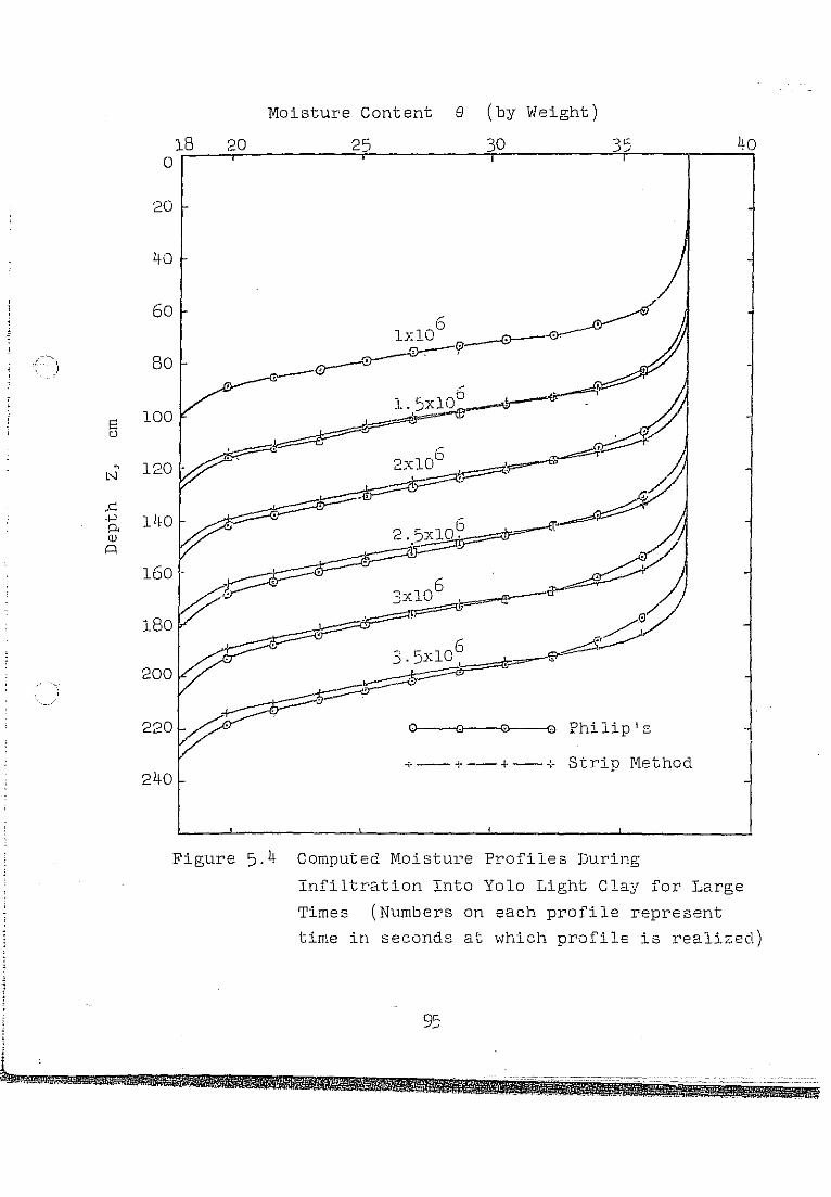
E: " ,
N
.c: -I-' p. OJ p
Moisture Content e (by Weight)
lS 20 25 30 35 40 0
20
40
60 6
lxlO ~(iI '. ,
So
6 100
1. 5xlO
~~ ,~. 6
120 - - - ') -10 ~X
140
160 - ~: ."
180 /0 3.5xlO~ ~' .,
200
220 ~ Philip I S
-i'--+--+--+ Strip Method 240
Figure 5.4 computed Moisture Profiles During
Infiltration Into Yolo Light Clay for Large
Times (N,®bers on each profile represent
time in seconds at which profile is realized)
95

i '
_1-... ;i! ;I, ; F ..
1t' ~ ;-~[ ,~ ;~J!~ ~ ~l
:;Ij; .,,'
-"6. CONCLUSIONS, DISCUSSIONS, AND FURTHER
RESEARCH POSSIBILITIES
6.1 TESTING THE RESULTS OF THE STRIP METHOD
In order to check the validity of the strip method, the
example of infiltration presented by Philip (1957c, p. 446)
is recomputed using the strip method procedure. The average
infiltration rate is calculated by dividing the area between
two successive moisture profiles of Figures 5.3 and 5.4 by
the increments of time. The comparative results are
-presented in Table 6.1 and are also shown in Figure 6.1. As
can be seen, the new approach gives results that correspond
closely to the Philip approach.
Referring to Figures 5.3 and 5.4 as time t increases
without limit, the strip method permits one to predict the
moisture profile which is approaching a constant shape
advancing down the column at a constant velocity_ In other
words, the infiltration capacity f is approaching a
constant value equal to saturated permeability (Ksat ) as
time goes
f c = Ksat
to infinity.
-6 = 12.3xlO
The line bc in Figure 6.1 represents
cm/sec , the asymptote to the
infiltration rate curve.
96
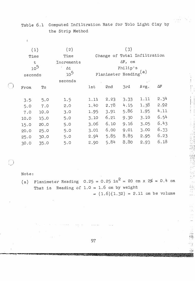
Table 6.1 Computed Infiltration Rate for Yolo Lj.ght Clay by
the Strip Method
( 1) ( 2) ( 3)
Time Time Change of Total Infiltration
t Increments iP, em
105 lit Philip's
seconds 105 Planimeter Reading(a)
seconds
From To 1st 2nd 3rd Avg.
3·5 5.0 1.5 1.11 2.23 3.33 1.11 2.34
5·0 7.0 2.0 1. 40 2.78 4.15 1.38 2·92
7.0 10.0 3.0 1.95 3.91 5.86 1.95 4.11
10"0 15.0 5.0 3.10 6.21 9.30 3.10 6.54
15·0 20.0 5·0 3.06 6.10 9.16 3.05 6.43
20.0 25.0 5.0 3.01 6.00 9.01 3·00 6 ?~ .~.)
25·0 30.0 5.0 2.94 5.85 8.85 2.95 6.23
30.0 35.0 5·0 2.90 5.81f 8.80 2.93 6.18
Note:
(a) Planimeter Reading 0.25 = 0.25 in2
= 20 em x 2% = 0.4 em
That is Reading of 1.0 = 1.6 em by weight
= (1.6)(1.32) = 2.11 em be volume
97
, . i
i
" , ··"1
111
i:,1

Table 6.1 (Continued)
( 4) Average Infiltration Rate
Strip Method 6F 106 em/sec f AVG = l'>t ) )
Planimeter Reading(a)
1st 2nd 3rd Avg. Philip I s Strip Method
1.13 2.2B 3.43 1.14 2.41 15.65 16.05 1. 44 2.90 4.33 1.44 3.04 14.60 15.20
1.99 4.00 6.01 2.00 4.22 13.70 14.05
3·17 6.32 9.47 3.16 6.66 13.10 13.35 3.10 6.20 9.29 3·09 6.53 12.B5 13.05
3.05 6.oB 9.12 3.04 6.40 12.65 12.Bo
3·00 5.98 B.95 2.98 6.30 12.45 12.60
2.96 5·91 B.BB 2.96 6.21f 12.35 12.50
98

CJ OJ
I.[) o rl X 'H
120 r.------.------.-----~------~----~---,
100
80 ..
'''-..., ~ ?o· -.-___ "____ .j
:~-________ -~-_-______ ~ ____ ._-_-__ ~ ______ ~ ________ ~~_a __ C_1 o ~
2xlO .....
Time t, seconds
Figure 6.la Infiltration Rate Curve for small times
(Depicted from Philip's 1957c, p. 446)
99
.------------~---------.-- ..... - - -

i5'F* FW
C)
OJ [JJ
"-5
=
IBr-______ ~------.--------.-------.--------r---,
17 .----.----.----. Philip's
16 ____ +-+-+ Strip Method
15
14
13-
Time t. seconds
Figure 6.1Q Computed Infiltration Rate Curve for
Large Times (point s a and b of Figure 6'.lb
correspond to a and b of Figure 6.1a)
100
..

6.2 COMMENTS ON THIS NEW APPROACH
The analysis presented here is idealized to the extent
that it is assumed the soil is unaffected by the physical
behavior of the texture, structure and characteristics of
the soil, and by the chemical content of the water passing
through it. The analysis also is for a homogeneous soil;
however, it could be modified for a layered soil, providing
the knowledge of the physical and hydraulic characteristics
--jf various layers are known.
In analyzing the strip method, one is able to take
advantage of computing the net movement (/',z) of the
position of any particular moisture content fJ during the
time interval (/',t) , instead of calculating moisture
increment (/',fJ) of this original moisture content fJ
during that time interval. Thus the soil moisture tension
and permeability of each section under consideration will
remain the same for successive time intervals. However, the
method introduces a slight error in depicting the moisture
profile after time interval (/',t) , since a straight line is
assmned to connect the extremities of adjoining strips.
Figure 6.2 is exaggerated in order to show the plotted
:.._)sitions of mOisture profiles. Meanwhile, the writer
believes that judicious selection of the length of time
interval will reduce both the computational error and time
without sacrificing accuracy.
The writer has made two runs using different time
intervals taking the initial moisture distribution at time
t = 3.5xl05 seconds as mentioned in Section 5.3. One run is
4 with equal time intervals of /',t = 1.OxlO seconds for 65
intervals; the other with unequal time intervals of
4 4 II /',t = 1.5xlO seconds, 2.0xlO seconds, and 3.0xlO· seconds
for the first, second, and last ten intervals. As can be
101
." ) , \

seen, the results presented in Table 5.5 and Figure 5.3 are
in very close agreement.
With respect to Philip's second paper (1957c), he has
stated that when time is very great his series solution of
Eq. (2.33) becomes unreliable. In his numerical example, he
pOints out when time t exceeds 5xl0 5 seconds, the solution
given by the first four terms of series Eq. (2.33) becomes
increasingly inaccurate. Therefore he used an alternative
method (1957c, p. 435-p. 448) involving a different approach
) to obtain the moisture profiles for large times (after
t = 5xl05 seconds). To supplement this occurrence the
writer has used Philip profiles at time t = 10xl05 seconds
as the second initial moisture distribution.
In applying the strip method one must start with a
known or assumed moisture profile. The development of the
moisture profile with time is entirely dependent upon the
physical characteristics of the medium, that is, the soil
moisture tension and permeability of the soil. Assumed
initial moisture distribution generally does not lead to a
good check with experimental work, because the physical
phenomena occuring during time interval (6t) are very
involved. Best results are obtained if the initial moisture
distribution is known.
102

___ --~ Mohture Content e
) ,
N
)
( M)
computed (M)
-----Y Plotted Moisture Profile
'~omputed Moisture Profile
Figure 6.2 Computed and Plotted Moisture
Distributions During Infiltration
103

6.3 SUGGESTIONS FOR FURTHER RESEARCH POSSIBILITIES
On the basis of the results of this dissertation there
are indications that, besides infiltration phenomenon, this
technique is also adaptable to problems of drainage and
upward ~low in soils induced by evaporation. Perhaps, one
of the more interesting and practical applications of the
strip method would be to apply it to other situations such
as evaporation from a soil after a period of infiltration.
Figure 6.3 shows that when infiltration ceases, the profile
development is characterized bya further penetration down
ward of the water front under the action of gravity and a
movement upward to the dry surface through evaporation. In
this case some means of adjusting the soil moisture tension
curve to account for variations in the wetting and drying
zones of the soil will have to be devised. Difficulty in
computation may arise at the dividing line between upward
and downward movement. However, it is anticipated that
further research should lead to the development of methods
permitting application to the field conditions, and it is
also hoped that further study will permit the use of this
approach in situations where initial soil moisture is not
Imown.
104

)
~ MOisture Content e
\ \ \
\3 \2 \
1
; \
\ \ \
\)) ~// s ~ /
'" / "
Figure 6.3 Moisture Movement in Soil During
Period of Evaporation
105
L.
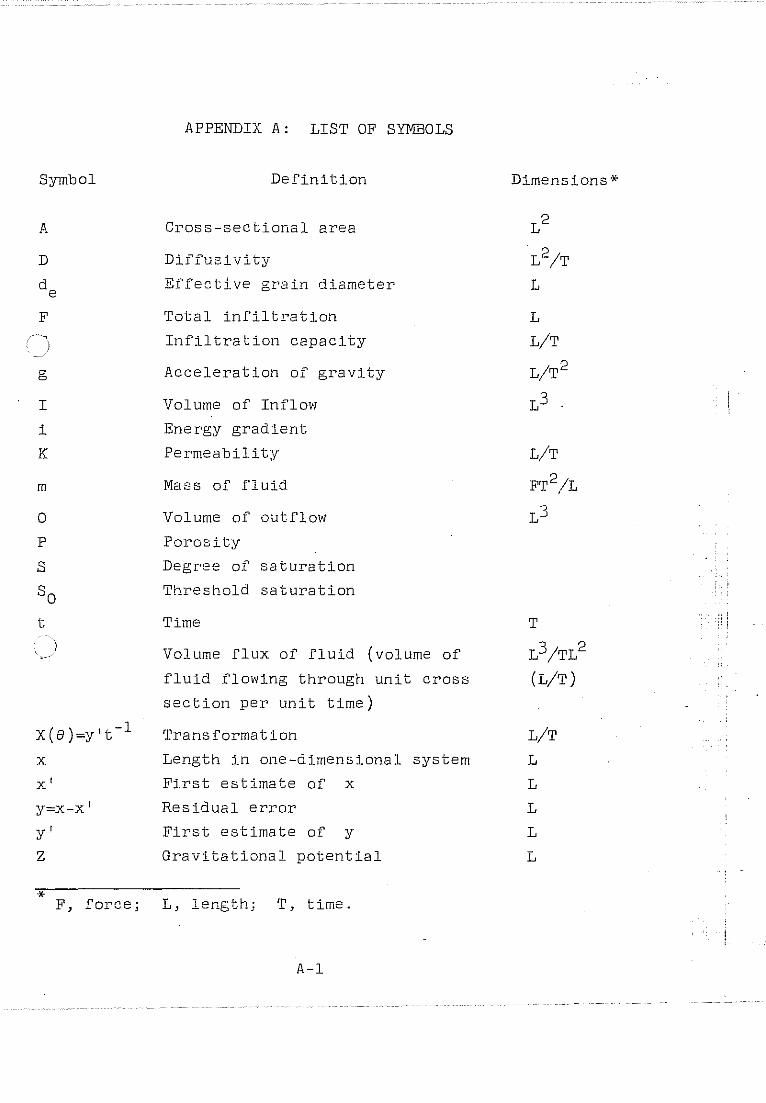
Symbol
A
D
g
I
i
K
m
)
X(B)=y't-1
x
x'
y=x-x'
y'
Z
*
APPENDIX A: LIST OF SYMBOLS
Definition
Cross-sectional area
Diffusivity
Effective grain diameter
Total infiltration
Infiltration capacity
Acceleration of gravity
Volume of Inflow
Energy gradient
Permeability
Mass of fluid
Volume of outflow
Porosity
Degree of saturation
Threshold saturation
Time
Volume flux of fluid (volume of
fluid flowing through unit cross
section per unit time)
Transformation
Length in one-dimensional system
First estimate of x
Residual error
First estimate of y
Gravitational potential
F, force; L, length; T, time.
A-I
Dimensions*
LIT
FT2/L .,
L.J
LIT
L
L
L
L
L
f !

Symbol
z
B
p
APPENDIX A (Continued)
Definition
Height of the strip
Unit weight of fluid
Change of storage
Movement of a section
Change of moisture content
Moisture content expressed in
volumetric terms
Dimensions
Inactive moisture content L3/L3
Initial mOisture content L3/L3
Threshold moisture content L3/L3
Moisture content on dry weight basis F/F
Dynamic viscosity FT/L2
Density of fluid FT 2/L 4
Bulk density on dry weight basis FT 2/L 4
Mass of fluid per total volume FT2/L4
Total potential L
Negative pressure (capillary
potential)
L
q,(B)=xt- l / 2 Boltzmann transformation
A-2

APPENDIX B: RESULTS OF COMPUTATIONS
B.l Computed MOisture Profiles for 65 Equal Time Intervals
of L1t = 1. OX104- seconds with Initial Moisture
Distribution at time t G
= 3.5xl05 seconds.
Section MOisture M=l(a) M=2 M=3 Content Depth Z
e em (by Weight)
1 37·.5 0.00 0.00 ·0.00 2 35·8 26·31 26.84- 27.38
3 34-.1 31.23 31·77 32.32 ~. 32.4 33·34- 33.89 34.4-5
5 30.6 35·36 35· 93 36·50 6 28.8 37.18 37.76 38.35
7 27.0 39.00 39.61 4-0.21
8 25·2 4-1·54- 4-2.18 4-2.81
9 23.4 4-4-.18 4-4-.85 4-5· 51 10 21. 6 4-6.30 4-7.00 4-7.68 'I:
. )ll ' .
19.8 ~8. 71 4-9.4-3 50.13 12 18.0 55·66 56 .42 57·17
Ii
Note: (a) M is the number of time intervals.
B-1

E.l (Continued)
M=4 M=5 M=6 M=7 M=8 M=9
0.00 0 .. 00 0.00 0.00 0.00 0.00
27.93 28·50 29.08 29.66 30.24 30.82 32.87 33.44 34.02 34.60 35·19 35· 78 35.01 35,58 36.16 36.75 37.34 37.93 37.08 37.66 38.24 38.83 39.42 40.02
("J 38.94 39.53 40,,12 40.72 41.31 41.91 ~
40.82 41.42 42.02 42.62 43.23 43.84 43.43 44.06 41f.68 45·30 45 .. 92 If6·54 46.16 ~6.81 47.45 48.09 48.73 49,,36 48.36 49.03 49.69 50.34 51.00 51.64 50.83 51 .52 52.20 52.88 53·55 54.22
57.92 58.66 59·39 60,12 60.84 61 .. 56
M=10 M=11 M=12 M=13 M=14 M=15
0.00 0.00 0.00 0.00 0.00. 0.00 31,41 32.00 32·59 33·19 33·79 34.39
.'-----.., 36.37 36.96 37·55 38.15 38.75 39.35 ;,,,j
38.52 39.11 3971 40.31 40.91 41. 51 40.61 41.21 41.81 42.41 43.02 43.62 42·52 43.12 43.72 44·33 44.93 45.54 44.45 45·05 45·66 46.27 46.89 47.50 47.17 If 7.78 48. 110 49·02 49.64 50.26 1[9.99 50.63 51.26 51.89 52·5:), 53.14 52.29 52.93 53·57 54 21 54.85 55. 49 54.88 55.54 56 .20 56 .85 57·50 58.15 62.27 62.98 63 68 64.38 65·08 65·77
H-"

B.l (Cant inued )
! ! , :
M=16 M=17 M=18 M=19 M=20 M=21 ,: i i , , , , : , ,
0.00 0.00 0.00 0.00 0.00 0.00 : ! ,
35. 00 35. 61 36.22 36.83 37.45 38.07 I
39.96 40·57 41.18 41.79 42.40 43.02
42.12 42.73 43.34 43.95 44·56 45·18 • i
44.23 44.84 45·45 46.06 46.67 47.29 ! !
.!+6.15 46.76 47.37 47,99 48.60 49.22 I l , ; ,
49.95 48.11 48.72 49.34 50·57 51.19 ! • 50.88 51·50 52 .12 52.74 53.36 53.98 ! .. 53.77 54.40 55·02 55.65 56.27 56 .90 !
a ~
56.12 58.02 58.65 56.75 57.39 59.28 , i
58.80 59.44 60.08 60.72 61.36 62.00 I ~ ~
66.46 67·14 67.83 68·51 69.19 69.86 1 • 1 i , : l
, , i i:;
! I ' ,
:_1 ii
M=24 M=26 '., ~
M=22 M=23 M=25 M=27 : : ~ ;-: OJ'
! ,: ~
0.00 0.00 0.00 0.00 0.00 0.00 iii i , , . '11 l
38.69 40.56 39.31 39·93 41.18 41.81 ."11 it
::ii ~
~3.64 44.26 44.88 45· 51 46.13 46.76 ' : ill , , " " " 't
45·79 46.41 47.03 47.65 48.28 48·90 :; i , j
47.91 48·52 49·14 49.77 50.39 51.01 ,:Ii!
jl 3 " i i'
49.83 50.45 51.07 51,69 52.31 52.94 I' ;
51.80 52.42 53.04 53.66 54.29 54.91 I· a , . :: :-
54.60 55. 22 55·84 56 .46 57·09 57.71 " Ii , :
"
57.52 58.15 58 .77 59.40 60.02 60.65 " I ;; , .
59.91 60·53 61.16 61.79 62.42 63.05 ' ~
·1 Iii " ~
62.64 63.27 63"91 64.54 65. 17 65·80 ,[ ... Ii !!, 'i
70·54 71.21 71.88 72·55 73·22 73.89 . ~
~
. ,~- -
.:' =-~:::..:-:..::
:,'." f'7; B-3 -;'
! L
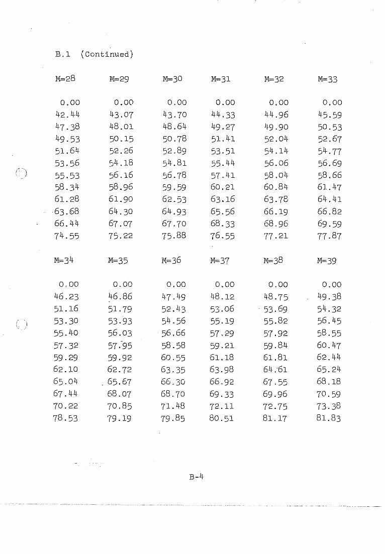
B.l (Continued)
M=28 M=29 M=30 M=31 M=32 M=33
0.00 0.00 0.00 0.00 0.00. 0.00 42.44 43.07 43.70 44.33 44.96 45.59 47.38 48.01 48.64 49.27 49.90 50.53 49.53 50.15 50.78 51.41 52.04 52.67 51.64 52.26 52.89 53.51 Sif.14 54.77 53.56 54.18 54.81 55.44 56.06 56.69 - . t ) 55.53 56.16 56.78 57.41 58.04 58.66 58.34 58.96 59.59 60.21 60.84 61.47 61.28 61.90 62.53 63.16 63.78 64.41 63.68 64.30 64.93 65.56 66.19 66.82 66.44 67.07 67.70 68.33 68.96 69.59 74.55 75.22 75.88 76.55 '{7.21 77.87
M=34 M=35 iVI= 36 lVI= 37 M=38 M=39
0.00 0.00 0.00 0.00 0.00 0.00 46.23 46.86 47.49 If8.12 48.75 49.38 51.16 51.79 52.43 53.06 53.69 54.32 53.30 53.93 54.56 55·19 55.82 56.45 55.40 56.03 56.66 57.29 57.92 58.55 57.32 57.95 58.58 59.21 59.84 60.47 59.29 59.92 60.55 61.18 61.81 62.44 62.10 62.72 63.35 63.98 64.61 65.24 65.04 . 65.67 66.30 66.92 67.55 68.18 67.44 68.07 68.70 69.33 69.96 70.59 70.22 70.85 71.48 72.11 72.75 73.38 78.53 79.19 79.85 80.51 81.17 81.83
B-4

B.l (Continued)
M=40 M=41 M=42 M=43 M=44 M=45
0.00 0.00 0.00 0.00 0.00 0.00 50.01 50.64 51. 27 51.90 52.53 53.16 54.95 55.58 56.21 56.84 57.47 58.10 57.08 57.71 . 58.34 58.97 59.60 60.23 59.18 59.81 60.44 61.07 61.70 62.33 61.10 61. 73 62.36 62.99 63.62 64.25 63.07 63.70 64.33 64.96 65.59 66.22 "~I
\..,j.87 66.50 67.13 67.76 68.39 69.02 68.81 69.44 70.07 70.70 71.33 71.96 71. 22 71.85 72.48 73.11 73.74 74.37 74.01 74.64 75.27 75.90 76.53 77.16 82.49 83.15 83.81 84.40 85.12 85.78
M=46 M=47 M=48 M=49 M=50 M=':;l
0.00 0.00 0.00 0.00 0.00 0.00
53·79 54.43 :; 5. 06 55.69 56.32 ':,6·95 .. ,
58.73 59.36 60.00 60.63 61.26 61.89 ' ::;
( \87 61. 50 62.13 62.76 6" 0'0 ---l' ..J~ 64.02 -
62.96 63.60 6~.23 64.86 65.49 66.12 64.88 65.51 66.14 66.77 67.40 68.04 66.85 67.48 68.11 68.74 69.37 70.01 69.65 70.28 70.91 71.54 72.17 72.80 72.59 73.23 73.86 74.49 75.12 75·75 75.00 75.63 76.26 76.89 77.53 78.16 7/.79 78.42 79.05 79.69 80.32 80.95 86.44 87.10 87.76 88.41 89.07 89.73
i !
B ---,

B.1 (Continued)
M=S2 M=S3 M=S4 M=5S M=56 M=S7
0.00 0.00 0.00 0.00 0.00 0.00
57. S8 S8.21 58.8S 59.48 60.11 60.74
62.52 63.1S 63.78 64.42 65.0S 65.68
64.65 6S.28 65.91 66.55 67.18 67.81
66.75 67.38 68.01 68.64 69.28 69.91
68.67 r9 ~n b .:)_ 69.9-3 70.56 71.19 71.82
70.64 71.27 71.90 72.53 73.16 73.79
73.44 74.07 74.70 75.33 75.96 76.59
76.38 77.01 77.64 78.27 78.90 79.54
78.79 79.41 80.05 80.68 81. 31 81.94
81.58 82.21 82.84 83.47 84.11 84.74
90.38 91.04 91.70 92.35 93.01 93.67
M=58 M=59 M=60 M=61 M=62 M=63
0.00 0.00 0.00 0.00 0.00 0.00
61.37 62.00 62.64 63.27 63.90 64.53
66.31 66.94 67.57 68.21 68.84 69.47
68.44 69.07 69.70 70.34 70.97 71.60 .
70.54 71.17 7L80 72.43 73 ·97 73.70
72.45 73.09 73.72 74.35 74.98 75.61
74.42 75.05 75.69 76.32 76.95 77 .58
77.22 77.85 78.49 79.l2 79.75 80.38
80.17 80.80 81.43 82.06 82.69 83.32
82.58 83.21 83.84 84.47 85.10 85.73
85.37 86.00 86.63 87.26 87.90 88.53
94.32 94.98 95.63 96.29 96.95 97.60

B.l ( Continued)
M=64 M=65
0.00 0.00 65.16 65.80 70.10 70.73 72.23 72.86 74.33 74.96 76.24 76.88 78.21 78.84 8l.01 8l.64 83.96 8 tl.59 86.37 87.00 89.16 89.79 98.26 98.91
B-7
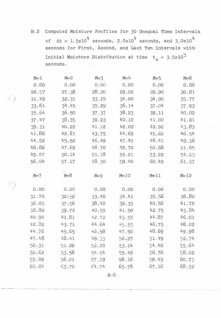
B.2 Computed Moisture Profiles for 30 Unequal Time Intervals
M=l
P.OO
26.57 3l.~9
33.61 35.6~
37 .~7 39·31 41.86 ~~.52
46.66 ~9.07
56.0~
M=7
0.00 31.70
j8.80 40.90 42,82
~)o. 31 52.62 55.22
~ ~ ~ of L'>t = 1.5xlO seconds, 2.0xlO seconds, and 3.0xlO
seconds for First, Second, and Last Ten Intervals with
Initial Moisture Distribution at time to = 3.5xl05
seconds.
0.00
27.38
32.31
34. ~5
36.50
~0.22
~2.8l
~5.52
4'r . 69 50. 1~ 57.17
0.00
32:59 37. ~,6 39.72 1~1. 81
43·71 ~5.65
48.41 51.26
53,58 56.21 63-,70
~'l= 3 0.0(:
28.20
33,15
35.29
37,37 39.23 ~1.12
~3.75
46,~9
48 70 . ,
51.18
"8 010 ./J,_,
0.00 33, lr6
38. ~2
~0.59
~~, 64
4/ "8 D.?
49.33
~,7 .19 64,74
B-8
M.=4
0.00 29.06
3~,00
36.14
38.23
40.12 ~2.02
~~.69
~7. ~5
49.70 52.21 59.40
jVl=lO
0.00 3~.~1
39.35 ~l. 50
~3, 59
~7.50
50.27 53.1~
55. 1r9 58.16
65·78
M=5
0.00 29.96 34.90
37.0~
39.11 ~l.OO
42.92 1+5.62 48.41 50.68
5'3.22
60.~9
M=11
0.00 35.56 ~O.~)6
~2,75
!r~ ,87
46.75 48.69 51. 49 54 . ~·o :;6.76 5,9.}+5
6'! .16
M=6
0.00 30.81
35.77 37.93
40.02
Ill. 91
113.83
~0,5~
lr9.36
51.65
ol. 57
M=12
0.00
36.80
~1.72
43.84 46.01 48.02 49.913
55.6~
')8.02 60.73 68,52

B.2 (Continued)
M=13 M=14 M=15 M=16 M=17 M=18
0.00 0.00 0.00 0.00 0.00 0.00
38.08 39.35 40.62 41.87 43.13 44.38
42.99 44.27 45.54 46.79 48.04 49.30
LI5.11 46:33 47·59 48.85 50.10 51. 36
Lf7·22 48.50 49.77 51.02 52.27 53.53
49.08 50.35 51.62 52.87 54.13 55.39
, , 51.13 52.40 53.66 54.90 56.15 57.41 I
54.01 55.14 56.38 57.63 58.88 60.14
56.90 58.16 59.37 60.61 61.86. 63.11
59.28 60.54 61. 79 63.02 64.27 65.52
62.01 63.28 64.55 65.80 67.06 68.31
69.88 71.22 72.57 73·90 75.22 76.54
M=19 M=20 M=21 M=22 M=23 M=2Lf
0.00 0.00 0.00 0.00 0.00 0.00
45.64 46.90 48.79 50.68 52.57 54.47
50.56 51.82 53.71 55.60 57.49 59.38
52.62 53.88 55.77 57.66 59.55 61. 4.4
54.79 56.05 57.94 59.83 61.71 63.60
56.64 57.90 59.79 61.68 63.58 65.47
58.66 59.92 61.81 63.70 65.59 67.47
61.40 62.66 64.55 66.44 68.33 70.22
64.37 65.63 67.52 69.41 71.30 73.19
66.78 68.04 69.93 71.82 73.71 75.60
69.57 70.83 72.72 74.61 76.50 78.39
77.86 79.17 81.15 83.12 85.09 87.06
B-9
1\
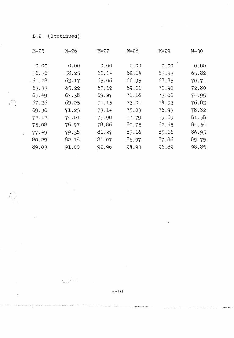
B.2 (Continued)
M=25 M=26 M=27 M=28 M=29 M=30
0.00 0.00 0.00 0.00 0.00 0.00 56.36 58.25 60.14 62.04 63.93 65.82
- 61. 28 63.17 65.06 66.95 68.85 70.74 63.33 65.22 67.12 69.01 70.90 72.80 65.49 67.38 69.27 71.16 73.06 74,,95 67.36 69.25 71.15 73.04 74.93 76.83 69,,36 71.25 73,,14 75,,03 76.93 78.82 72.12 74.01 75.90 77.79 79.69 81. 58 75.08 76.97 78.86 80.75 82.65 84.54 77 .49 79.38 81.27 83.16 85.06 86.95 80.29 82.18 84.07 85.97 87.86 89.75 89.03 91.00 92.96 94.93 96.89 98.85
B-10


71$ mow = 7""-7'""P' rt _~_
B.3 (Continued)
M=13 M=14 M=15 M=16 M=17 M=18
0.00 0.00 0.00 0.00 0.00 0.00
91.49 93.97 96.44 98.92 10l. 40 103.88 96.49 98.97 101. 44 103.92 106 .. 40 108.88 99.01 101.48 103496 106.44 108 .. 92 lll. 40
101.94 104.42 106.89 109.37 111.85 114.33 104 .. 10 106.57 109.05 111.53 114.01 ll6.49 107.17 109.65 112 .. 12 ll4.60 117.08 ll9.56 110 .. 42 ll2.90 115.38 117.86 120.33 122.81 ll4.46 ll6.94 119.41 12l.89 124.37 126.85
117·55 120.03 122" 50 124.98 127 .. 46 129.94 121.19 123.67 126.14 128.62 131.10 133.58 133.00 135.54 138.08 140 .. 62 143.16 145.70
M=19 M=20 M=21 . M=22 M=23 M=2 1! .
0.00 0.00 0.,00 0.00 0.00 0 .. 00 106.::16 10S.84 111.32 113.80 116.28 ll8.76 111.36 113.84 116.32 118.80 12l. 28 123.76 113.88 l16,35 l1S.83 12l. 31 123.79 126.28 116.81 119.29 121.77 124 .. 25 126.73 129.21 ll8.96 121.44 123.92 126.40 128.88 13l. 37 122.04 124.52 127.00 129.48 13l.96 134.44 125.29 127.77 130.25 132.73 135·21 137.69 129.33 13l.81 134.29 136.77 139.25 14l. 73 132.42 131f.90 137.3'3 l39.S6 I 1f2.34 144.32 136.06 1:.S.54 141. 02 143.50 145.98 148.46 148.24 150.78 153.31 155.S5 158.39 160.93
f',-12
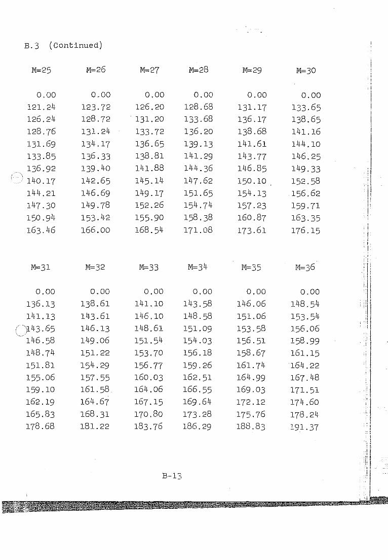
B.3 (continued)
M=25 M=26 M=27 M=28 M=29 M=30
0.00 0.00 0.00 0.00 0.00 0.00 121.24 123.72 126.20 128.68 131.17 133.65 126.24 128.72 . 131. 20 133.68 136.17 138.65 128.76 131.24 133.72 136.20 138.68 141.16 131. 69 134.17 136.65 139.13 141.61 144.10 133.85 136.33 138.81 141.29 143.77 146.25 136.92 139. ~O 141.88 144.36 11r6.85 149.33 ,!
140.17 142.65 145.14 147.62 150.10 , 152.58 , I,
144.21 146.69 149.17 151.65 154.13 156.62 i I ! i
147.30 149.78 152.26 154.74 157.23 159.71 1 ' I·
150.91l 153.42 155.90 158.38 160.87 163.35 i ,
163.46 166.00 168.54 171.08 173.61 176.15 ' , i :
. I
! , , M=31 M=32 M=33 M=34 M=35 M=36 ,:/ :
, , , , ,I
0.00 0.00 0.00 0.00 0.00 0.00 "
I 136.13 138.61 141.10 143.58 146.06 148.54 !I 141.13 11r3.61 146.10 148.58 151.06 153.54 I
I "I
\14~ 65 ,.. 5· 146.13 148.61 151.09 153.58 156.06 i
146.58 149.06 151.54 154.03 156.51 158.99 148.74 151.22 153.70 156.18 158.67 161.15 151.81 154.29 156.77 159.26 161.74 164.22 155.06 157.55 160.03 162.51 164.99 167.48 159.10 161.58 164.06 166.55 169.03 171. 51 162.19 164.67 167.15 169.64 172.12 174.60
q 165.83 168.31 170.80 173.28 175.76 178.24 iI
178.68 181.22 183.76 186.29 188.83 191.37
B~13

B.3 (Continued)
M=37 M=38 M=39 M=40 M=41 M=42
0.00 0.00 0.00 0.00 0.00 0.00 1:;1.03 153.51 155.99 158.48 160.96 163.44 156.03 IS8.51 16099 163.48 165.96 168.44 1:18. 51~ 1(:::l.O3 163.51 165.99 168.48 170.96 161.48 163 .. 96 166.41~ 168.93 171.~1 173.89 163.63 166.12 168.60 171.08 173.::1 176.05 166.71 169.19 171. 67 1"4,16 176.61'1 179.12 169.96 172.44 IH.93 1""0'7 4' ! f' .L 179.89 182.38 17~.00 176.4e "L 7S 96 . . ,- 181. 11)+ 183.93 186.41 177 .09 179.57 182.05 184.54 187.02 189.50 180.73 183.21 IB5 .. 69 18e.le 190.66 193.11[
193·90 196.44 198.97 201. Sl 20 lL04 206.58
M=43 11']=44 lVl=, 4 5 JVl=46 M=47 lV1=11.8
0.00 0.00 0.00 0.00 0.00 0.00 ') 165.93 168.41 i'--' ",..., ,'1 .. I .O;i 173.38 175.86 178.34
170.93 173.41 ]75.89 1'78.38 180.86 183.34 1"'" 44 - I -' - 175.93 178.41 180.89 183.38 1.9S.e6 176.38 178.86 181.34 183.83 186.31 188.79 178.53 181.02 183.50 1.95.98 188.47 190,95 18l. 61 181[.09 le6.57 189.06 191.54 194.02 184.86 187,,3 1+ 189.83 192.31 194.79 197.28 IBe.90 191.38 193.86 196.35 198.83 201. 31 19l. 99 1911.47 196.95 199.44 201.92 204.40 195.63 198.11 200.59 203.08 205.56 208.04 209.12 211e65 214,19 21tJ.72 219,26 221.79

E.3 (Continued)
M=49 M=50
0.00 0.00
lS0.S3 lS3.31
185.83 lSS.31 lSS.34 190.83 191.28 193.76
193.43 195.92
.. 196 .51 198.99 . 199.76 202.24
203.S0 206.23
206.S9 209.37 210.53 213.01 221, . 33 226.86
( )
B-15
, "
I I I
: I I ,
i'
i i
I I ! I I
. I
i I I I
i i! !
, I " !
l I

APPENDIX C: BIBLIOGRAPHY
1. Ashcroft, G., Marsh, D. D., Evans, D. D., and Boersma, L., 1962, Numerical Method for Solving the Diffusion Equation: I. Horizontal Flow in Semi-Infinite Media. Soi~ SCi. Soc. Amer. Pree., Vol. 26, No.6: 522-525.
2. Auten, J. T., 1934, The Effect of Forest Burning and Pasturing in tbe Ozarks on the Water Absorption of Forest Soils, U.S. Dept. Agr. Fores~ Service, Central States Forest Exp. Sta, Note 16.
3. Baver, L. D., 1959, Soil Physics, John Wiley and Sons, Inc., New York, Ttlird Edi ti on: 81- 303.
4, Bodman, G. B., 1938., The Variability of the Permeability Constant at Low HydrBulic GradlentE During Saturated Water Flow in Soils Soil Sci. Soc. Amer. Proc. 2: 45-53.
5. Bodman, G. B., and Colman, E. A., 1944, MOisture and Energy Condltions During Downward Entry of Water into Soils. Soil Sci. Soc. Amer. Proc, 8: 116-122.
6. Buckingham, E., 1907, Studies on the Movement of Soil Moisture. U.S. Dept. Agr. Bur. Soils, Bul. 38: 1-61.
7. Childs, E. C .• 1956, Recent Advances in the Study of Water Movement in Unsaturated Soil. Trans. Intern. Congr. Soil Sci. 6th Congr. 39: 265-274.
8. Childs, E. C" and George, N .. C., 1950, The Permeability of Porous Materials. Proc. Roy. Soc. (London), 210A: 392-399.
9.
10.
Fireman, ~" 1944, Permeability Measurements on Disturbed Soil Samples.. Soil SCi., 58: 337-353 ..
Gardner, Tests of in Soil.
W .. R .. , and Mayhugh, M. s., 1958, Solutions the Diffusion Equation for the Movement of SolI Sci. Soc .. Amer. Proc., 22: 197-201.
and Water
11. Haines. W. E., 1923, The Volume-Change AssOCiated with Variations of Water in Soil. J. Agr. Sci., 13: 296-310.
12. Horton, R. E., 1933, Tbe Role of Infiltration in the Hydrologic Cycle. Trans. Amer Geophys. Union, Vol. 14: ~46-460.
13. Irmay, S., 195~, On the Hydraulic Conductivity of Unsaturated Soils, Trans. Amer. Geophys. Union, Vol. 35: 463-467.
C-l
. , ,
: I I I ,

BIBLIOGRAPHY (Continued)
14. Klute, A", 1951, Some Theoretical Aspects of the Flow of Water in Unsaturated Soils. Soil Sci. Soc. Amer. Proc., 16: 144-148.
15, Klute, A., 1952, A Numerical Method for Solving the Flow Equation for Water in Unsaturated Materials. Soil Sci. 73: 105-116 .
16. Linsley, Ray K., and Franzini, Joseph B" 1955, Elements of Hydraulic Engineering. McGraw-Hill Book Company, New York, 486-523,
17. Linsley, Ray K., Kohler, Max A., and Paulhus, Joseph L. H., 1958, Hydrology for Engineers. McGraw-Hill Book Company, Inc., New York, 122-148.
18. Linsley, Ray K., Kohler, Max A., and Paulhus, Joseph L. H., 1949, Applied Hydrology. McGraw-Hill Book Company, Inc., New York, 283-315.
19. Martin, J. p" and Waksman, S. A., 1940, Influence of Micro-Organisms in Soil Aggregation and Erosion, Soil Sci., 50: 29-47.
20. Moore, R. E., 1939, Water Conduction f-rom Shallow Water Tables. Hilgardia, 12: 383-426.
21. Nielsen, D. R., Biggar, J. W .. , and DaVidson, J. M." 1961, The Prediction of Soil Water Movement Based on a Diffusion Equation, First Annual Report, Univ. of Calif., DaViS, Calif.
22. Philip, J. R~, 1955, Numerical Solution of Equations of the Diffusion Type with Diffusivity ConcentrationDependent. Trans. Faraday Soc., 51: 885-892.
23. Philip, J. R., 1957a, The Theory of Infiltration: 1. The Infiltration Equation and Its Solution. Soil SCi., 83: 345-357-
24. Philip, J. R., 1957c, The Theory of Infiltration: 2. The Profile of Infinity. Soil Sci., 83: 435-448.
25. Philip, J. R., 1957d, The Theory of Infiltration: 3. MOisture Profiles and Relation to Experiment, Soil SCi., 84: 163-178,
C-2

BIBLIOGRAPHY (Continued)
26. Philip, J. R., 1957e, The Theory of Infiltration: 4. Sorptivity and Algebraic Infiltration Equations. Soil Sci., 84: 257-264.
27. Quirk, J. P., and Schofield, R. K., 1955. The Effect of Electrolyte Concentration on Soil Permeability. Jour. Soil Sci., 6: 163-178.
28. Richards, L. A., 1931, Capillary Conduction of Liquids in Porous Mediums. Physics, 1: 318-333.
29. Richards, L. A., 1955, Retention and Transmission of Water in Soil. United States Salinity Lab., Riverside, Calif., Yearbook of Agr .. , Separate No. 2580: 144-151.
30. Richards, L. A., and Richards, S. J., 1957, Soil Moisture. United States Salinity Lab., Riverside, Calif., Yearbook of Agr., Separate No. 2788: 49-60.
31. Russell, M. B., 1942, The Utility of the Energy Concept of Soil Moisture. Soil Sci. Soc. Amer. Proc., 7: 90-94.
32. Schofield, R. K., 1935, The pF of the Water in Soil. Trans. Third Inter. Congr. Soil Sci., Vol. 2: 37-48.
33. Sherwood, G. E. F., and Taylor, A. E., Calculus. Revised Edition, p. 478, Prentice-Hall.
34. Todd, David K., 1959, Ground Water Hydrology. John Wiley and Sons, New York, 14-77.
35. Veihmeyer, F. J., and Edlefsen, N. E., 1937, Interpretation of Soil Moisture Problems by means of EnergyChanges. Trans. Amer. Geophys. Union, 18: 302-318.
36. Watson, K. K., 1958, Infiltration Studies with Particular Reference to Infiltrometer Experiments on a Small Rural Catchment. Thesis submitted to New South Wales University of Technology, 185-193.
37. Youngs, E. G., 1957, Moisture Profiles During Vertical Infiltration. Agr. Research Council Unit of Soil Physics, Cambridge, England, 283-290.
C-3