AN ANTITRUST ANALYSIS OF BUNDLED LOYALTY DISCOUNTS

by Patrick Greenleea David Reitmanb David S. Sibleyc

October 30, 2006

Abstract Consider a monopolist in one market that faces competition in a second market. Bundled loyalty

discounts, in which customers receive a price break on the monopoly good in exchange for making all

purchases from the monopolist, have ambiguous welfare effects. To analyze such discounts as predatory

pricing is incorrect. In some settings, they act as tie-in sales. Existing tests for whether such discounts

violate Section 2 of the Sherman Act do not track changes in consumer surplus or total surplus. We

present a new test and use it in an illustrative example based on SmithKline that assumes the “tied” market

is a homogeneous good. If the tied market is characterized by Hotelling competition, bundling by the

monopolist causes the rival firm to reduce its price. In numerical examples, we find that this can deter

entry or induce exit.

JEL Code: L42 Keywords: market share discount; bundling; tying; predation ___________ aU.S. Department of Justice, 600 E Street NW, Suite 10000, Washington DC 20530, USA

patrick.greenlee@usdoj.gov. Corresponding author. ph: 001-202-307-3745, fx: 001-202-514-5847. bCRA International, 1201 F Street NW, Suite 700, Washington DC 20004, USA, dreitman@crai.com

cEconomics Department, University of Texas at Austin, 1 University Station #C3100, Austin TX 78712,

USA, dsibley@ersgroup.com

This is an updated version of EAG Discussion Paper 04-2, February 2004. We thank Dennis Carlton,

Einer Elhauge, Ken Hendricks, Barry Nalebuff, Alex Raskovich, and Greg Werden for helpful comments,

as well as Sarah Dolnick and Shameek Sinha for excellent research assistance. The views expressed

herein are solely those of the authors and do not represent the views of the United States Department of

Justice.

1

I. INTRODUCTION

Bundled loyalty discounts provide price breaks on one or more products to buyers that remain

sufficiently loyal to a supplier. They resemble volume discounts in that shifting incremental purchases

from a rival supplier may allow a buyer to satisfy a loyalty requirement and thereby enjoy lower prices.

They resemble tying when affordable prices for one (tying) product are available only to consumers that

are completely loyal to the supplier in their purchases of a second (tied) product. Like volume discounts

and tying, bundled loyalty discounts can enhance or diminish consumer surplus and total welfare by

improving the ability to price discriminate, and they can change the long run incentives for single-product

firms to enter/exit. Open questions include under what conditions should competition authorities treat

bundled loyalty discounts like tying or predatory pricing, and when do bundled rebates enhance welfare.

Bundled loyalty discounts have recently received considerable attention in antitrust circles in light

of LePage’s, Inc. et al. v. 3M Company,1 Michelin v. Commission,2 and a number of pending court cases. 3

Until recently, the practice of bundled rebates has received comparatively little scholarly and judicial

scrutiny. Indeed, only a small number of cases litigated in the U.S. have focused squarely on these

practices, including SmithKline Corp. v. Eli Lilly & Co.4 and Ortho Diagnostics Sys., Inc. v. Abbott Lab,

Inc.5 Virgin Atlantic Airways Ltd. v. British Airways PLC6 involved similar practices, but the district court

found allegations of anticompetitive behavior to be unsupported by fact. LePage’s provides a good

background for the issues involved.

The facts in LePage’s begin with the very strong brand name of Scotch tape, a 3M product. Most

retail merchants believed that they had to offer Scotch tape. Until the early 1990’s, 3M’s share of the U.S.

1 324 F.3d 141 (3rd Cir. 2003). 2 Case T-203/01 Manufacture francaise des pneumatiques Michelin v Commission [2003] ECR II-4071. 3 See, for example, reports on litigation involving pharmaceuticals (Hensley 2004 and Pollack 2005) and microprocessors (Parloff 2006), as well as Antitrust Modernization Commission (2005), European Commission (2005), and the commentary of Ahlborn and Bailey (2006). 4 427 F. Supp 1089, 1094 (E.D.PA.1976); 1976 U.S. Dist. LEXIS 12486j 1976-2 Trade Cas. (CCH), P61, 199. 5 920 F. Supp. 455 (1996). 6 257 F. 3d 256 (2001). A similar lawsuit was litigated in Europe: Case IV/D-2/34.780.

2

market for transparent and invisible tape exceeded 90%. Starting in the early 1990’s, however, 3M’s share

began to erode with the rise of office superstores such as Staples and Office Depot. These retailers sold

products, including tape, under their own names as private labels. LePage’s dominated the growing

private label segment, with an 88% market share in 1992. Its share of the overall tape market, however,

was only 14%.

3M responded by adding a private label of its own, under the Highland name. 3M’s entry

involved the use of a bundled rebate program that “offered discounts to certain customers conditioned on

purchases spanning” multiple product lines, with the size of the rebate depending on the extent to which

the customer met growth targets established by 3M. 3M’s bundled discounts apparently proved successful

in shifting a large fraction of private label tape business to 3M. In 1992, LePage’s filed a four-count

antitrust suit against 3M that was ultimately narrowed to a monopolization claim under Section 2 of the

Sherman Act. 7 LePage’s argued that it was foreclosed from selling private label tape because it could not

cover its costs and still compensate customers for the rebates lost on other products in the discount

program when the customer bought private label tape from LePage’s instead of from 3M.

The legal strategy of the defendant, 3M, was to compare price to cost and use the case law of

predation. It argued that as long as the price of each item in its bundle exceeded cost, the pricing scheme

was legal. In other words, 3M argued that the relevant case law was that of predatory pricing, as presented

in Brooke Group.8 In its appellate filings, 3M used a different approach, the Ortho test. In Ortho, the

defendant offered bundled discounts on products,9 some of which were competitive and some of which

were monopoly products due to patents. The Court allocated the total bundle rebate to the competitive

product in question and compared that globally discounted price to the defendant’s cost. This approach

effectively adapted Brooke Group to the analysis of bundled discounts. According to this test, if the

7 One of the four counts was exclusive dealing. The jury found against LePage’s on this claim. 8 Brooke Group Ltd. v. Brown & Williamson Tobacco Corp. 509 U.S. 209 (1993). 9 In the context of these cases, bundling refers to a set of discount prices that are only available if the relevant products are bought largely or entirely from the dominant multi-product firm. This differs from the standard usage in economics, where bundling refers to the sale of a set number of units of various goods.

3

discount-adjusted price of the competitive product exceeds its cost, then the bundled discount pricing

strategy is deemed not anti-competitive.

The great interest in LePage’s probably stems from the fact that bundled rebates are a widespread

business practice. Until LePage’s, the Ortho test was an accepted way of analyzing bundled discounts.

The Court of Appeals’ decision in LePage’s, however, leaves matters in doubt. To quote the U.S.

Department of Justice:

…The court of appeals was unclear as to what aspect of bundled rebates constituted exclusionary conduct, and neither it nor other courts have definitively resolved what legal principles and economic analyses should control. 10 Employing a bundled loyalty discount imposes switching costs on customers because a customer

that shifts some purchases to a rival seller pays a higher unit price for the quantity still purchased from the

incumbent. In VAA/BA, Virgin Atlantic proposed an incremental sales test to judge the legality of such

pricing plans. This test compares the competitor’s incremental revenue from making those new sales to

the customer to the competitor’s incremental cost. Because the competitor must compensate the customer

for the switching cost, net incremental revenue may be forced below incremental cost. In such a setting,

“incremental” competition is unprofitable and is deterred by the loyalty discount plan. The VAA/BA test

simply checks whether net incremental revenue exceeds incremental cost, and if it does, the loyalty

discount plan is presumed legal. Like Ortho, this test analyzes bundled rebates using predation case law.

The academic economics literature on bundled discounts is rather sparse. Bundling for the

purpose of price discrimination has a large literature, but usually in a monopoly setting. The main

exception is Nalebuff (2004a), who has written extensively on how bundling can be used to reduce

competition. Discounts that apply to every unit purchased have a smaller literature. Kolay, Shaffer, and

Ordover (2004) examine a monopolist’s use of all-units discounts on a single product, and compare them

to menus of two-part tariffs. Greenlee and Reitman (2004) analyze loyalty discounts, both with and

without bundling. In a duopoly differentiated products setting in which both firms can offer a loyalty 10 Brief for the United States as Amicus Curiae, 3M Company FKA Minnesota Mining and Manufacturing Company, Petitioners, and LePage’s Incorporated, et al. On Petition for a Writ of Certiorari to the United States Court of Appeals for the Third Circuit, at 8.

4

program to a retailer that sells to consumers with varying tastes, they show that firms pass the VAA/BA

test in equilibrium. Thus failing the VAA/BA test suggests that a firm has goals other than short-term

profit maximization. In a setting similar to LePage’s, they show that the introduction of bundled discounts

causes standalone prices to rise. The welfare effects of bundled rebates in Greenlee and Reitman (2004)

are ambiguous, since their models allow for price discrimination across consumer types. 11 Nalebuff

(2004b, 2005) together contain results similar to Theorems 1 and 2 below, under the assumption that the

tied market is perfectly competitive. We relax this assumption in part of our analysis.

From the standpoint of antitrust enforcement, it is unclear what body of case law best applies to

bundled discounts. The approaches of the Ortho test and the VAA/BA incremental test suggest that

bundled rebates should be analyzed as a method of predation. In LePage’s, 3M argued vigorously in its

appellate briefs that its discounts were legal under Brooke Group because even its discounted prices were

above cost, an assertion not challenged by the plaintiff.

However, because the intent of bundling is to induce consumers to buy multiple products from a

single seller, perhaps tying is a more appropriate way to look at bundled discounts. Indeed, the Third

Circuit suggested this in LePage’s, but went no further. It is worth noting that in LePage’s and in Ortho,

the firm offering the loyalty program included in the bundle a product over which it had either a

monopoly (Ortho, due to patents) or a very strong brand name (Scotch tape, in LePage’s). Monopoly

goods within the bundle, then, may play the role of tying products. As we show below, however, bundled

discounts are not always equivalent to tying.

While our focus is on the short term competitive effects of bundled loyalty discounts, a full

analysis of bundled rebates would also consider the longer term implications as new competitors

contemplate entry and/or incumbent competitors consider exit. Similar to tying, bundled rebates can

change the terms on which firms compete in the linked market. As we will discuss, however, the manner

in which bundled rebates influence the dynamics of competition differ from the effects of tying. 11 Their model includes small consumers that are not eligible for a loyalty program. Small consumers are always harmed by the introduction of a loyalty program, but this loss may be balanced by surplus gains to large consumers. For alternative analyses and commentary, see also Carlton (2001) and Tom et al. (2000).

5

To summarize, this paper provides preliminary answers to two main questions. First, what is the

correct legal framework to use in the antitrust analysis of bundled loyalty discounts? Second, how can one

distinguish between bundled discounts that benefit consumers from ones that do not?

We reach the following conclusions.

• When the tied market is perfectly competitive, bundled discounts resemble tying and are not a

form of predatory pricing.

• Bundled discounts can raise or lower consumer welfare. In either case, equally efficient

competitors may be foreclosed. Profit-maximizing bundled discounts lower consumer surplus

when the tied market is perfectly competitive.

• If products in the tied market are homogeneous, simple price comparison tests exist that can

distinguish bundled rebates that raise consumer surplus from those that do not.

• These tests, applied to SmithKline, suggest that the bundled discounts at issue there probably

lowered consumer surplus and total surplus.

• If the rivalrous market is a differentiated product duopoly rather than characterized by

homogeneous goods, bundled discounts are not equivalent to tying. In such cases, profit-

maximizing loyalty programs have ambiguous welfare effects, and aggregate consumer surplus

can rise or fall due to bundling. This suggests that bundled discounts should not always be

analyzed as tying arrangements.

• In the differentiated product setting, bundled discounts reduce rents for the non-bundling firm.

Numerical examples indicate that bundled discounts can deter entry or induce exit.

The remainder of this article is organized in the following manner. Section II introduces our base

model of a monopolist in one market that faces perfect competition in a second market. Sections III and

IV discuss existing tests of bundled discounts and introduce a generalized test. Section V applies this test

to SmithKline. Section VI briefly looks at nonlinear pricing and establishes that a monopolist benefits

6

from offering a menu of bundled “three-part tariffs” that is not feasible without bundling. Section VII

modifies the initial model by making the second market a differentiated duopoly. Section VIII concludes.

II. MODEL 1: PERFECT COMPETITION IN THE LINKED MARKET

Firm 1 has a monopoly in market A and is one of many perfect competitors in market B. For each

consumer, demands are economically independent and described by ( )AA PQ and ( )BB PQ . All

consumers demand B, though some consumers may have zero demand for A at any positive price. Non-

zero demands are assumed to be downward sloping. As in LePage’s, firm 1 signs a contract with each

consumer that specifies bundled rebates, or fails to do so. Absent signing a contract, the consumer buys A

at the standalone price and B at marginal cost.

Let ( )ii PCS be consumer surplus, where ( ) ( )iiii PQPSC −=′ , BAi ,= . Denote by AP the

choke price for market A, given by ( ){ }0inf =AAA PQP , and let *AP and *

BP be the standalone monopoly

prices in markets A and B. Firm A has constant marginal cost Ac for A and all firms have constant

marginal cost Bc for B.

An important assumption throughout is that consumer surplus is positive in market A at the

monopoly price. This rules out the possibility that firm 1 extracts the entire consumer surplus via a two-

part tariff. Less-than-full rent extraction can occur for a variety of reasons including contract

incompleteness and demand uncertainty. When contracts cannot completely specify the terms of

exchange, the joint surplus of the supplier and retailer depends on the parties’ relative bargaining power,

so rent extraction typically is less than complete.12 When demand for the monopoly product is stochastic,

the optimal two-part tariff does not extract all expected surplus from market A. Under this interpretation,

( )AA PQ can be thought of as an expected demand curve and ( )AA PCS as expected consumer surplus. 13

12 Consult Iyer and Villas-Boas (2003), including their discussion of the empirical study of branded tuna pricing by Kadiyali et al. (2000). 13 See Mathewson and Winter (1997) and Brown and Sibley (1986). We address demand uncertainty in Section VI.

7

To establish terminology, a price pair ( )BA PP , is a bundled loyalty discount if it is available to

consumers only on the condition that they buy everything from firm 1. Firm 1 also sets a standalone price

for A, which a consumer pays if he or she buys B from a competitor. The price of A in the bundle is

discounted from the standalone price. We imagine an initial situation in which firm 1 prices

independently across markets, setting prices at ( )BA cP ,* . Subsequently, firm 1 offers a bundled discount

plan, consisting of bundled prices and a standalone price for A. This paper studies the effects of this

pricing innovation.

We consider, in turn, independent pricing by the monopolist and a loyalty program that consists

of a standalone price AP and a price pair ( )BAA PP ,ε− . A consumer that participates in the loyalty

program receives an Aε discount on all its purchase of A whenever it agrees to make all of its B

purchases (at price BB cP > ) from firm 1. Faced with these alternatives, the consumer decides whether to

participate in the bundled rebate program and makes purchases accordingly.

A. Pareto-Improving Bundled Rebates

One theme of this article is that bundled rebates, with or without a share-based loyalty feature,

can improve or harm welfare. To see how welfare may increase, suppose that initially there is

independent pricing, firm 1 charges *AP for A and Bc for B. Firm 1 can construct another pair of prices

consisting of a slightly discounted price of A and a price of B slightly above Bc . We can write this price

pair as ( )BAA PP ,* ε− . For BP close enough to Bc , consumers prefer this pair to ( )BA cP ,* . Furthermore,

since the effect of Aε on profits is second-order, but that of BB cP − is first-order, firm 1’s profit

increases. If firm 1 makes ( )BAA PP ,* ε− available only to consumers who buy entirely from firm 1, then

( )BAA PP ,* ε− is a bundled rebate. Note that because the consumer prefers the bundled rebate to the initial

(and still available) prices, an equally efficient competitor cannot make sales of B at price equal to Bc .

8

To develop intuition, we first consider introducing bundled rebates ( )BA PP , under the

assumption that the standalone price for A remains at the monopoly level. In the subsection that follows

this initial development, we allow the monopolist also to adjust the standalone price. When the standalone

price remains at the monopoly level, the optimal loyalty discount program ( )BA PP , maximizes firm 1

profit subject to the constraint that consumer surplus at ( )BA PP , weakly exceeds consumer surplus at

( )BA cP ,* . Formally, the monopolist’s objective is to

{ }BA PP ,Maximize ( ) ( )BBAA PP ππ + (1)

subject to: ( ) ( ) ( ) ( )BBAABBAA cCSPCSPCSPCS +≥+ *

Without loss of generality, we assume that if the incentive compatibility restraint is met with

equality, the consumer selects the bundled rebate program.

Theorem 1: [Pareto Improvement] Letting ( )BA PP , denote the optimal program prices, the solution to (1)

has the following features:

(1) ( ) ( ) ( ) ( )BBAABBAA cCSPCSPCSPCS +=+ * .

(2) ( ) ( ) ( ) ( )BBAABBAA cPPP ππππ +>+ * .

(3) Total surplus at ( )BA PP , exceeds total surplus at ( )BA cP ,* .

(4) *iii PPc << , BAi ,= .

(5) Equally efficient competitors are foreclosed in market B.

Proof. See Appendix.

This theorem has three implications. First, it shows that the effect of bundled rebates for antitrust

analysis is not akin to predation. Not only do AP and BP exceed marginal cost, but there is no short run

profit sacrifice, as called for by Brooke Group. Nevertheless, equally efficient competitors are foreclosed:

9

the lost discount on A exceeds the benefit received from obtaining B at price Bc instead of BP . Second,

although foreclosure is often discussed as reducing welfare, this need not hold for bundled rebates. Third,

bundled rebates are equivalent to tie-in sales in this setting. The “standalone” price *AP serves only to

induce consumers to select the bundled prices and buy everything from firm 1.

B. Monopoly Extension Using Bundled Rebates

We now consider how bundled rebates can extend monopoly from A to B. Firm 1 sets a

standalone price for A, AP , a discount Aε , and also sets a price BP for B. The prices ( )BAA PP ,ε− are

only available if the consumer buys everything from firm 1. Otherwise, the consumer pays AP to buy A

from firm 1 and buys B from a competitor at price Bc . Firm 1’s objective is to

{ }BAA PP ,,Maximize

ε ( ) ( )BBAAA PP πεπ +− (2)

subject to: ( ) ( ) ( ) ( )BBAABBAAA cCSPCSPCSPCS +≥+− ε

Observe that in this setting, the standalone price AP can be set arbitrarily high provided that Aε increases

in a similar fashion. As AA PP ˆ→ , ( ) 0→AA PCS and the incentive compatibility constraint in this

problem converges to that of a straight requirements tying problem. 14

If ( ) ( ) ( )BBBBAA cCSPCSPCS ≥+ ** then the constraint above is slack at the optimum. The

bundled rebate is ( )** , BA PP and AP ( )AAP ε+= * can be set so that

( ) ( ) ( ) ( ){ }PCScCSPCSPCSPP ABBBBAAA ≥−+≥ ** inf (3)

If ( ) ( ) ( )BBBBAA cCSPCSPCS <+ ** then the constraint binds at the optimum and A AP ε− and BP are set

below their monopoly levels. In equilibrium, AA PP ˆ≥ in order to relax the incentive constraint as much

14 This does not hold for less competitive settings like the differentiated products setting we study in Section VII, or when there are small consumers that cannot qualify for any loyalty discount program as in Greenlee and Reitman (2004).

10

as possible. With this, the problem is akin to a requirements tying problem, but monopoly extension is not

complete. The following theorem summarizes this discussion.

Theorem 2: [Monopoly Extension] Consider the loyalty discount ( )BAAA PPP ,, ε− .

(i) If ( ) ( ) ( )BBBBAA cCSPCSPCS >+ ** , then *AAA PP =− ε , *

BB PP = , and

( ) ( ) ( ) ( ){ }PCScCSPCSPCSPP ABBBBAAA ≥−+≥ **inf .

(ii) If ( ) ( ) ( )BBBBAA cCSPCSPCS <+ ** , then *AAA PP <− ε , *

BBB PPc << , and AA PP ˆ≥ .

Notice that equally efficient competitors are foreclosed again, and employing a bundled rebate reduces

consumer welfare. In Theorem 2.i, total surplus declines because the bundled rebate generates a

deadweight loss in B and no change in A.

Note that in Theorem 2.ii, where ( ) ( ) ( )BBBBAA cCSPCSPCS <+ ** , the profit maximizing price

of A, AAP ε− , is below the initial monopoly price, *AP . One might conjecture that consumer welfare

increases because the effective price of A has fallen. For Theorem 2.ii, however, the optimal prices

constrain consumer welfare to equal ( )BB cCS . In contrast, consumer welfare equals

( ) ( ) ( )BBAABB cCSPCScCS >+ * under independent pricing. Hence, using a bundled rebate reduces

consumer welfare, even though the price of A has fallen.

The total surplus effect of bundled discounts, however, is ambiguous. Compared to the

independent prices ( )BA cP ,* , in Theorem 2.ii the bundled price of A is lower and that of B is higher.

Hence, total surplus rises or falls depending on the relative market demands. The following corollary

provides additional precision for the case of linear demands in both markets.

Corollary 1. Suppose demands and costs are linear in both markets.

11

(i) Theorem 2.i corresponds to the inequality: ( ) ( )BBAA cCScCS 3≥ .

(ii) If ( ) ( ) ( )BBAABB cCScCScCS 39

16 <≤ , then Theorem 2.ii applies and bundled discounts

lower total surplus.

(iii) If ( ) ( )BBAA cCScCS9

16< , then Theorem 2.ii applies and bundled discounts increase

total surplus.

Proof: See Appendix.

For ease of exposition, we have assumed no uncertainty in the demand curves for A and B. With

this modeling simplification, bundled discounts are unnecessary whenever the monopolist can set a two-

part tariff that extracts all surplus in A. As Mathewson and Winter (1997) establish, however, tying can

improve profits when demands for A and B are uncertain but correlated. With stochastic demand, the

optimal two-part tariff does not extract all surplus in A, and tying allows the monopolist to flexibly extract

additional consumer surplus when demand is high. In Section VI, we introduce uncertainty by having the

consumer’s demand be a random variable (high or low) whose realization is unobserved by firms. If

demand realizations for A and B satisfy non-crossing and uniform ordering properties, then firm 1 earns

strictly greater profit when it offers a menu of bundled “three-part tariffs” (consisting of an entry fee, a

discounted price for A, and a discounted price for B) than when it offers a menu of separate two-part

tariffs for A and prices competitively in B. Thus with demand uncertainty, bundled discounts are not

redundant to a monopolist that can offer two-part tariffs. 15

The purpose of stating Theorems 1 and 2 separately is to provide a means of distinguishing

bundled rebate plans that lower consumer welfare from those that do not. For example, one could

compare the effective price of the monopoly good in the bundle to its price under a pre-existing

independent pricing regime. If there is no difference, then the bundled rebate plan cannot be Pareto-

15 Mathewson and Winter (1997) establish this for a monopolist that offers a single three-part tariff to all consumer types. In Section VI, we show this for a monopolist that offers a menu of three-part tariffs to a population of two customer types. See also Sibley and Srinagesh (1997) and Iyer and Villas-Boas (2003).

12

improving, since Pareto-improving discount plans involve at least a small reduction in the price of the

monopoly good (Theorem 1). Such a pattern of no price change for A would be consistent with Theorem

2.i. If the price of A in the bundle is lower than the pre-existing independent price, this is consistent with

both Theorem 1 and Theorem 2. To distinguish between them, compare the standalone prices. Under

Theorem 1, the standalone price is simply the pre-existing monopoly price, while under Theorem 2.ii the

equilibrium standalone price is higher. The only cases left to consider involve the standalone price being

less than *AP , which is not optimal for firm 1. Thus, even though the bundle price of B is above marginal

cost, the net consumer effect is seen just by comparing AP and *AP .16 Naturally, applying these tests

requires price data for well-defined periods preceding and following the introduction of bundled rebates.

One may object that Theorem 1 is of little relevance because the monopolist can increase its

profits by raising the standalone price above the initial monopoly price. The implication is that one would

never expect to see a standalone price no higher than the pre-bundling monopoly price. One response is

that, nonetheless, firms may behave in this manner. 3M, for example, claimed consistently that its

bundled discount prices were all lower that its pre-bundling prices and that the standalone prices were

simply the pre-bundling prices, with subsequent adjustments for cost increases. 17 At a minimum, if Model

1 applies, the condition *AA PP ≤ could be used as a safe harbor in antitrust enforcement.18

III. EXISTING TESTS OF BUNDLED REBATES

As argued above, bundled rebates are not equivalent to predation, so the case law involving

Brooke Group is unlikely to be directly useful in antitrust enforcement. Rather, for settings resembling

Model 1, bundled rebates are best viewed as a form of tie-in sale. That said, the case law on tying does

16 It would be tempting to apply this test to LePage’s. Unfortunately, the prices required are not available in the public record. For a discussion, including the approach presented here, consult Rubinfeld (2005). 17 See Rubinfeld (2005:253). 18 Of course, a shrewd monopolist may initially set its monopoly price artificially high in order to reach such a safe harbor after introducing a bundled loyalty discount program.

13

not provide convenient rule of reason tests for the competitive effects of bundled rebates, and tying often

has ambiguous welfare effects.

One test described above is the Ortho test. In our terminology, the Ortho test would ask whether

firm 1’s revenues from B less the discounts on A cover its costs of B. If so, then the bundled rebates plan

is presumed legal. 19 One problem with this test is that it assumes disequilibrium behavior. That is, if it is

passed, why has not a market B competitor already undercut the bundle?20

Alternatively, competitors may have higher costs than firm 1, so that they cannot undercut in

market B. This implies a different underlying model than the present one, and it is not clear that antitrust

attention is warranted when rivals have higher costs. Thus, if the Ortho test is passed by firm 1, but rivals

in market B cannot undercut firm 1’s price in market B, their lack of success may not result from firm 1’s

pricing, but from their own cost disadvantages.

A second point to keep in mind is that a bundled discount program can fail the Ortho test yet still

raise consumer surplus. 21 Consider again the intuit ion behind Theorem 1. Suppose the monopolist offers a

loyalty discount program that prices A slightly below *AP and B at marginal cost. To a first order,

monopolist profits have not fallen and the consumer strictly prefers facing ( )BAA cP ,* ε− rather than

( )BA cP ,* . Thus, total welfare and consumer welfare have risen. However, even for Aε extremely small, a

perfect competitor in B cannot “pay” the consumer Aε and still earn a non-negative profit. For these two

reasons, the Ortho test cannot detect consumer surplus or total surplus changes. Nonetheless, it can be

used as a safe harbor test.22

19 This test is equivalent to determining whether pricing for A and B under the bundled rebate is “compensatory” as introduced by Ordover and Willig (1981). Ordover served as an economic expert for the plaintiff in Ortho. See also Nalebuff (2004c). 20 The test that we propose above, though, has a similar theoretical problem: any bundled discount plan that passes it, given Theorem 1, cannot be maximizing profits. 21 In this respect, the Ortho test once again resembles cost tests for predation. 22 For more on how both our test and the Ortho test can be used as a safe harbor for legitimate conduct, see Greenlee and Reitman (2005).

14

The VAA/BA incremental profit test also merits discussion. Share-based discounts can exist within

a bundle of prices or can apply to an unbundled single product. Parsing the term “bundled rebates,” it

appears that for homogenous goods it is the bundling of discounted prices that has importance for

competition, not whether the discounted prices within the bundle are share-based. While a loyalty

discount program may make it unprofitable for equally efficient competitors to win incremental business,

such firms can compete effectively for the consumer’s entire requirements. Thus, with homogenous

products, a bundled discount program can flunk the VAA/BA test, yet not reduce competition, consumer

surplus, or total surplus. Hence, the usefulness of the VAA/BA incremental test in the present context

appears limited.23 By contrast, the price comparisons described above involve equilibrium prices and can

distinguish bundled rebates that raise consumer welfare from those that lower it. Neither the Ortho test

nor the VAA/BA test can do this, even in principle.

IV. EXTENSIONS AND VARIATIONS OF MODEL 1

A. Non-Independent Demands

Our discussion has assumed independent demands for A and B. This facilitates characterizing the

optimal bundled and standalone prices. For the more limited (but still important) purpose of determining

whether a newly introduced bundled discount strategy raises or lowers consumer surplus, we do not need

this assumption.

Suppose that the introduction of a bundled discount causes no change in the price of B. If the

standalone price of A, AP , is no higher than the pre-bundling monopoly price, then the outside options

available to consumers are no worse than before the introduction of the bundled rebate. Consumer surplus

cannot decline following the introduction of such a program. Clearly, this requires no special assumptions

about whether A and B are complements, substitutes, or are independent.

23 However, as mentioned above, if products are differentiated and buyers prefer a mix of products from multiple firms, then the VAA/BA incremental test can distinguish short run profit maximizing behavior from potentially exclusionary behavior. See Greenlee and Reitman (2004, 2005).

15

Suppose, alternatively, that the standalone price of A rises with the introduction of the bundled

rebate. Since the price of B cannot fall below Bc in equilibrium, this implies that the outside options

available to consumers are less desirable than the initial prices *AP and Bc . The loyalty program that

maximizes firm 1 profit makes the consumer indifferent between the bundle rebate prices ( ),A A BP Pε−

and the standalone prices ( ),A BP c . Hence, if *A AP P> then introducing the bundled rebate reduces

consumer surplus. Thus, assuming that firm 1 maximizes profits, we have a test to determine how

bundled loyalty discounts affect consumer surplus: if *A AP P≤ , consumer surplus weakly increases, and if

*A AP P> , consumer surplus diminishes.

As a practical matter, one should sound a cautionary note about the second part of the test. To

infer consumer harm from observing *A AP P> requires that firm 1 comes close to actually maximizing

profits. If the firm fails to maximize profits, it could be true that *A A AP Pε− < and BB cP = , but

*A AP P> . Clearly, the consumer benefits, but since *

A AP P> , our proposed test would suggest otherwise.

Hence, before using *A AP P> to infer anything, the analyst should try to verify that the bundling firm is

maximizing profits. Alternatively, if the bundled price is sufficiently high that *A A AP Pε− > , then the

bundled discount unambiguously diminishes consumer surplus and total surplus. This qualification does

not affect the positive inference to be made when *AA PP ≤ .

B. Two Firms in the Competitive Market

So far, we have assumed that the non-monopoly market is perfectly competitive. This assumption

ensured that the equilibrium prices of firm 1’s market B rivals are not affected by firm 1’s pricing

strategy. Nothing changes if there is only one market B rival, provided that the B products are

16

homogeneous and firms can set prices for B-only customers that differ from the bundle price for B.24 The

equilibrium in such cases has firm 1 setting loyalty program prices in a manner that makes the consumer

indifferent between accepting the program and purchasing only B at cost, and firm 2 (the sole market B

rival) setting price at marginal cost.

The duopoly results change if the firms cannot distinguish consumers that purchase A and B from

those that purchase only B, or if the firms cannot prevent resale. Here, we briefly discuss how the analysis

changes for this version of our first model, and examine it more deeply in a differentiated products setting

in Section VII. With the assumption of homogenous goods, both firms price B at marginal cost in

equilibrium absent a loyalty discount program. Introducing a bundled loyalty discount can only cause

firm 1’s price of B to rise, and firm 2 may respond optimally by increasing its price. In such instances, a

test in the spirit of the above is still useful. If the standalone price of A under bundling is higher than the

pre-bundling monopoly price of A, then Theorem 2 implies that consumer surplus falls, even if firm 2

prices at marginal cost. To the extent that firm 2 raises its price, that conclusion is reinforced. On the

other hand, if the standalone price is not greater than the pre-bundling monopoly price, we can no longer

conclude that consumer surplus has declined.

C. Effects on Entry and Exit

The result of firm 1’s introduction of bundled rebates has, from one perspective, a dramatic

impact on firm 2: rival firms are foreclosed from serving consumers who buy both A and B. Nevertheless,

the model’s assumptions imply much less stark effects in the long term. Given the assumption of perfect

competition and constant marginal costs in market B, firms enter only when they have no fixed costs. To

the extent that there are consumers who buy only in market B, rival firms still operate in the B market and

earn normal profit. Thus for this model, bundled rebates have no additional adverse impact on

competition given the potential for entry.

In fact, as discussed above, if the B market is a duopoly prior to the introduction of bundled

rebates, and firms cannot distinguish A-and-B consumers from B-only consumers, then the use of bundled

24 An equivalent assumption would be that there are no consumers that purchase only B.

17

rebates increases profits not only for firm 1 but also for its rival. Taking this one step further, suppose that

firm 1 initially has a monopoly in markets A and B, and faces a potential entrant in market B. Absent

bundling, the prospect of intense competition deters entry whenever the potential entrant has positive

entry costs. If firm 1 uses bundled rebates, however, the potential entrant will earn positive operating

profit and thus enters when it has sufficiently small entry costs. Thus, while bundled rebates foreclose an

entrant from part of the market, such a pricing strategy may induce entry by increasing the profits

available to the potential entrant.

V. SMITHKLINE RECONSIDERED

An example of how our test can be applied is provided by SmithKline.25 Lilly was the sole U.S.

supplier of the cephalosporin family of antibiotics, introducing it in 1964 under the brand name Keflin.

Subsequently, Lilly introduced three other cephalosporins, under the brand names Keflex, Loridine and

Kafocin. Lilly had U.S. patents and exclusive rights for each of these drugs, and was the sole U.S.

supplier of cephalosporins until October 1973. At that time, SmithKline entered the cephalosporin market

with a drug called Ancef, obtained from a U.S. patent owner under a non-exclusive license. About a

month later, Lilly introduced Kefzol, an antibiotic generically equivalent (and thus a direct competitor) to

Ancef. To show how our test can be applied, we assume that Ancef and Kefzol are perfect substitutes.

Prior to entry by SmithKline, Lilly had offered volume-related rebates, as part of a Cephalosporin

Savings Plan (CSP). In the latter half of 1974, Lilly examined ways to combat SmithKline, and on April

1, 1975, it introduced a Revised CSP that reduced the discount to hospitals by about 3%. At the same

time, the new pricing plan gave an additional 3% rebate on a hospital’s total cephalosporin purchases

provided the hospital bought certain minimum quantities, specific to each hospital, for any three of Lilly’s

five cephalosporin drugs. 26

25 Nalebuff (2005) and Kobayashi (2005) also discuss SmithKline from the standpoint of the Ortho test. 26 See Opinion, in SmithKline, ibid Findings of Fact, paragraph 90. SmithKline argued that the total effect of the revised CSP was that “Hospitals allegedly receive approximately the same aggregate rebate under the revised CSP as that paid under the CSP.” See Opinion, p. 27.

18

From this discussion, the main elements of SmithKline roughly coincide with the assumptions of

our model. Lilly had monopoly cephalosporin products in the Revised CSP bundle and offered a discount

on the bundle. Lilly’s Kefzol and SmithKline’s Ancef were generically equivalent and, we assume,

perfectly homogeneous. 27

The Court calculated return on sales for Ancef assuming that SmithKline matched Lilly’s bundled

rebates. Assuming that SmithKline produced Ancef as efficiently as Lilly made Kefzol, the Court found

that SmithKline could not match Lilly’s bundled rebates without incurring losses. 28 That is, an equally

efficient competitor of Kefzol (or Ancef) could not have been profitable against the Revised CSP. The

Court found that Lilly had willfully maintained monopoly power under Section 2 of the Sherman Act, but

found that Lilly’s pricing practices did not constitute tying, under Section 1. Thus, the Court used the

Ortho test as a “bright line” test to determine whether or not Lilly’s rebates were anticompetitive.

Based on our analysis, Lilly’s bundled prices probably reduced consumer surplus and total

surplus. Because the 3% loyalty discount on Lilly’s bundle was cancelled out by the roughly 3%

reduction in volume-related rebates, a customer that bought the same quantity of the Lilly monopoly

products under the Revised CSP as under the original CSP would have paid the same price either way. In

our terminology, letting A refer to Lilly’s monopoly goods, AAA PP ε+= * , where *AP is the monopoly

price prior to the Revised CSP. In other words, the standalone prices of Lilly’s monopoly goods rose

under the Revised CSP and the discounted price with the loyalty rebates was approximately the same as

under the original CSP. By the argument in the previous section, even if the price of Ancef rose due to

Lilly’s bundling, we can conclude that the Lilly pricing strategy likely reduced consumer surplus.

Furthermore, since there was no change in the price paid for the monopoly products, and the price paid

for Kefzol rose, we can also conclude that total surplus declined. The Revised CSP would have the

27 This, along with an assumption that no hospitals purchased only the Kefzol/Ancef products, enables us to apply the test. If Ancef and Kefzol were not regarded as perfect substitutes by customers, then this analysis would not apply. 28 See Opinion, paragraph 110.

19

desired effect of lowering SmithKline’s sales of Ancef and preserving profits on Lilly’s cephalosporins

even if the price for Kefzol were somewhat above that for Ancef.29

Even though the SmithKline decision was correct, our analysis suggests that its reasoning could

have yielded a perverse welfare result. When the SmithKline court based its conclusion on the negative

margin calculation for an equally efficient supplier of Kefzol (or Ancef), it employed the Ortho test. The

Court correctly concluded that the Revised CSP foreclosed SmithKline. However, if the Revised CSP did

not include higher standalone prices for the monopoly products, consumer surplus and total surplus would

not have fallen (Theorem 1), yet an equally efficient competitor would have been foreclosed. Thus, the

SmithKline reasoning can generate incorrect inferences about the welfare effects of bundled rebates.30

VI. BUNDLED DISCOUNTS AND NONLINEAR PRICES

We assumed above that positive consumer surplus exists in market A at the monopoly price. We

deferred discussion of two-part tariffs and other types of nonlinear prices, partly on grounds of

convenience. In some cases, two part tariffs may allow the monopolist to extract consumer surplus in

market 1 completely. However, total surplus extraction is unlikely to be feasible in most cases. 31

Consistent with this is the fact that bundled discounts are often used without an entry fee, e.g. the

SmithKline case discussed above. In this section we demonstrate that optimal nonlinear prices often leave

positive expected consumer surplus, and that linking markets via a loyalty discount program enhances

profits, even when a monopolist otherwise can offer separate nonlinear prices for each good.

29 As the Court noted, “So long as its price on Kefzol was equal to or not much higher than Smith-Kline’s, Lilly counted on its reputation with physicians (particularly surgeons) and the reluctance of hospitals to suffer a decline in rebates (as compared with the rebates previously received under the CSP) because of their failure to participate in the Revised CSP, as a strategy to achieve its domination (goal of 75%) of the cefazolin market.” Opinion, paragraph 101. 30 The Third Circuit Court, which affirmed the lower court decision on appeal, came closer to the standard advocated here. The decisive factor in that opinion was that more competition, and with it lower prices, would have prevailed but for the bundled rebate scheme. 575 F. 2nd 1056 (3d Cir 1978.) 31 See the analysis in Iyer and Villas-Boas (2003) as well as Mathewson and Winter (1997).

20

Suppose that a consumer’s demand curve depends on a binary random variable, which can be

“low” (L) or “high” (H) with equal probability. Let ( )PQsi denote demand for good i in state s, and

assume that ( ) ( )PQPQ LAHA > and ( ) ( )PQPQ LBHB > whenever demand is positive. When A and B are

priced independently, competition in B makes nonlinear pricing infeasible: in equilibrium both firms price

B at marginal cost and charge no entry fee.

In market A, however, firm 1 has monopoly power and can design nonlinear prices that

discriminate between the two consumer types, subject to incentive-compatibility (IC) and individual

rationality (IR) constraints. For intuitive appeal, think of nonlinear prices as sets of optional two-part

tariffs. Let ( )EPCS ik , denote the consumer surplus of a type i consumer in market k who faces a two-

part tariff with entry fee E and usage charge P. The consumer knows the realized state of nature at the

time of contracting, but firm 1 does not.

Firm 1 sets the two-part tariffs for A in order to:

{ }( ) ( )[ ]∑

=

−+H

LiiAiAAiAiAPEPE

PQcPEHAHALALA

21

,,, Maximize (4)

subject to:

( ) ( )jAjAiAiAiAiA PECSPECS ,, ≥ (IC)

( ) 0, ≥iAiAiA PECS (IR)

where },{, HLji ∈ . Familiar manipulation generates the following nonlinear prices:

AHA cP = (5)

( ) ( )( )( )LALA

LALALAHAALA PQ

PQPQcP

′−−

+= (6)

∫∞

=LAP

LALA dPQE (7)

21

∫+=LA

A

P

cHALAHA dPQEE (8)

Note that ex ante expected consumer surplus in A is positive, so there is an opportunity to increase profit

by linking the two markets.

How would bundling work in this setting? Define the standalone price as the two-part tariff

( )AA cE ,ˆ , where AE can be made as large as desired. Thus, the consumer can purchase B at Bc and pay

AAA QcE +ˆ for A, if that consumer buys B from a rival of firm 1. Firm 1 offers consumers the choice of

two pricing plans ( )LBLALL PPET ,,≡ and ( )HBHAHH PPET ,,≡ , or the outside option of purchasing A at

the standalone price. For notational simplicity, define

( ) ( )∫∞

≡P

ikik dvvQPv .

A type L consumer enjoys surplus of ( ) ( )LA LA LB LB Lv P v P E+ − when it selects ( ), ,L LA LBE P P .

Firm 1 sets LT and HT to maximize expected profits, subject to two incentive compatibility

constraints (IC) and two indiv idual rationality constraints (IR).

{ }( ) ( )∑ ∑

= =

−+H

Li

B

AkikikkikiTT

PQcPEHL

Maximize 21

, (9)

subject to:

( ) ( ) ( ) ( ) jjBiBjAiAiiBiBiAiA EPvPvEPvPv −+≥−+ (IC')

( ) ( ) ( )[ ] ( )BiBAAiAiiBiBiAiA cvEcvEPvPv +−≥−+ ˆ,0max (IR')

for },{, HLji ∈ .

The right hand side of the individual rationality constraints sums the consumer surplus achieved

by purchasing A at the standalone price (or foregoing A altogether) and the consumer surplus generated by

buying B from a rival of firm 1. Observe that the standalone price AE appears only on the right hand side

22

of the individual rationality constraints. At a solution, AE is set to weakly exceed ( )ALA cv , just as the

linear pricing case where the optimal standalone price AP was set at least as large as the choke price AP .

Diminishing the outside option in this fashion relaxes the individual rationality constraints as much as

possible. In equilibrium, consumers always satisfy a discount plan instead of purchasing A at AP .

In a separating solution, AHA cP = , BHB cP = , and kLk cP > , BAk ,= .32 The entry fees LE and

HE extract consumer surplus fully from type L and make type H indifferent between LT and HT . Thus,

the gain to firm 1 from offering a bundled loyalty discount is that second-degree price discrimination in

market B now becomes feasible. Note also that expected consumer surplus remains positive. If type H’s

IR' constraint does not bind, then the nonlinear prices in markets A and B are the ones that separate

monopolists would set in each market. This is the nonlinear pricing version of Theorem 2.i, implying that

consumer surplus and total surplus decline.

Since the optimal unbundled prices in (5) – (8) are a feasible outcome of the bundling problem,

the monopolist earns higher profits by bundling than by using optimal unbundled two-part tariffs, given

the ex ante information constraint. In terms of an upper bound on profits, from (IR') consumer surplus for

each type must be at least as large as would be obtained by buying only product B at marginal cost. This

implies that the bundled profits cannot exceed the entire surplus from each type in market A. Thus, the

gain to bundling is at most the difference between consumer surplus in the A market at marginal cost

pricing and the ex ante unbundled monopoly profits in the A market. This result formally establishes the

intuition that the gains to bundled loyalty discounts are limited to what could be gained by improved

nonlinear pricing in the monopoly market. This discussion has demonstrated that whether prices are linear

or nonlinear, bundling can improve profits by expanding the scope for nonlinear pricing into market B. 32 The necessary and sufficient condition for the existence of a separating solution to the bundled nonlinear pricing problem is that there exist positive numbers eA and eB that satisfy:

( ) ( ) ( )[ ] 0>−+−+ ∫∫++ kk

k

kk

k

c

cLkHk

c

cLkkkLkk dPPQPQdPQcQ

εε

εε for }.,{ BAk ∈

23

VII. MODEL 2: IMPERFECT COMPETITION IN THE LINKED MARKET

The clean-cut nature of our welfare results thus far has depended on the assumption that market B

features homogeneous goods. In this section, we relax this assumption and suppose that market B is

served by duopolists that compete in a differentiated product environment. As we will show, the

equivalence between tying and bundled rebates evaporates in this setting as bundled rebates take on

additional facets of price discrimination.

Consumer preferences for B are uniformly distributed on the unit interval. Firm 1 is located at

zero and firm 2 at one. For firm i’s product, a consumer experiences a disutility k per unit of distance

between the consumer’s ideal point and firm i’s location. Denote by ( )PvB consumer surplus in the

market for B gross of this cost, k. Hence, if a particular consumer’s tastes are given by [ ]1,0∈t , net

consumer surplus from buying B from firm 1 at price 1P is ( )1Bv P kt− , while net consumer surplus from

buying B from firm 2 at price 2P is ( ) ( )2 1Bv P k t− − . Consumers with t values near zero prefer firm 1

while those with t near 1 prefer firm 2.

Of the unit population of consumers in the B market, a fixed fraction ,θ uniformly distributed on

the unit interval, also consume A. Thus, some A consumers prefer to buy B from firm 1 and others prefer

to buy B from firm 2. As we show below, not all A consumers will buy B from firm 1 in order to obtain a

discount on A. Some A-and-B consumers prefer firm 2’s product so strongly that they will pay the

(higher) standalone price for A. We assume that all A consumers buy B, either from firm 1 or from firm 2.

In effect, there are two consumer segments: θ that have positive utility for both A and B, and θ−1 that

have positive utility only for B.

As before, we denote the price of A in the bundle by AAP ε− and the standalone price by AP .

Firm 1’s price for B is 1P . Initially, we assume that firm 1 cannot charge a different price for B to bundle

customers than to non-bundle customers due to arbitrage possibilities, or because firm 1 cannot prevent

bundle customers from emulating non-bundle customers in the B market (perhaps by operating a separate

24

division). As it is not in firm 1’s interests to charge a lower price for both A and B to bundled customers,

firm 1 charges 1P to both types of customers. Later we discuss what happens if this assumption is relaxed

so that firm 1 charges different B prices to bundle and non-bundle customers. Firm 2’s uniform price for

B is 2P .

A. Pre-Bundling

Prior to bundling, firm 1 charges the monopoly price of A, *AP , and competes with firm 2 in the

market for B. Firm 1’s share of market B is given by

( ) ( )1 2

112 2

B Bv P v Pt

k−

= + , (10)

and firm 1’s profit is

( ) ( ) ( ) ( ) ( ) ( )1 21 1 1

12 2

B BA A A A B B

v P v PP c q P P c q P

kπ θ

− = ⋅ − + − ⋅ +

. (11)

Firm 2’s profit is

( ) ( ) ( ) ( )2 12 2 2

12 2

B BB B

v P v PP c q P

kπ

− = − +

. (12)

Note from (11) and (12) that prior to bundling, prices in B are set without regard to market A, and

that firm 1’s optimal price of A does not depend on the prices for B. Therefore, in equilibrium, firm 1

charges the monopoly price for A, and both firms set the Hotelling prices in B, that is if *P solves

( ) ( ) ( ) ( ) ( ) ( )****** PqcPPvPqPqcP BBBBBB −⋅′−=+′− then *21 PPP == .

B. Bundled loyalty discounts

With bundled pricing, the A and B markets interact. First, consider firm 1’s share of consumers

who buy A and B. Denoting this share by ABt , it is given by the expression:

( ) ( ) ( ) ( )1 212 2

A A A A A B BAB

v P v P v P v Pt

kε− − + −

= + . (13)

25

Of the population of B consumers that never purchase A, firm 1’s share, 0Bt , is given by the same

expression as prior to bundling:

( ) ( )1 20

12 2

B BB

v P v Pt

k−

= + (14)

Thus, firm 1 serves ABt ⋅θ consumers that have positive utility for both A and B and ( ) 0 1 Btθ−

consumers who demand only B.

Given this notation, there are ABt θ consumers that buy A and B at the bundled prices

( )1,A AP Pε− from firm 1. The mass of consumers who buy B from firm 2 and pay the standalone price

for A is given by ( )ABt−⋅ 1θ . Of the 1 – ? B-only consumers, ( ) 0 1 Btθ− buy B from firm 1 and

( ) ( )011 Bt−⋅−θ from firm 2.

With these definitions, firm 1’s profit when it offers a bundled discount program is

( ) ( ) ( ) ( )[ ]( ) ( ) ( ) ( ) ( ) ( )110

111

1 1

PqcPtPqcPtPqcPPqcPt

BBBAAAAAB

BBAAAAAAAB

−⋅−+−⋅−⋅+−+−−−⋅⋅=

θθεεθπ

(15)

Firm 2’s profit when firm 1 bundles is

( )( ) ( ) ( )( )( ) ( )220222 11 1 PqcPtPqcPt BBBBBAB −−−+−−= θθπ (16)

As a preliminary matter, note that the standalone price of A plays a different role with bundling

than it did in Model 1. In Model 1, the only function of the standalone price is to induce consumers of A

and B to buy solely via the discount program. This explains the equivalence of bundled discounts and

tying in Model 1. AP plays a similar role in Model 2, but it is also a price at which some sales may occur,

to A consumers who have a strong preference for firm 2 in the B market. If AP is set to make 0=AQ

outside the bundle, some consumers may still buy B from firm 2. Hence, firm 1 does better by setting AP

low enough that it can profit from selling A to consumers with strong preferences for firm 2 (t close to 1).

Comparing 1P to *P , intuition suggests that for bundled discounts to be profitable, the program

price of B must be higher than the price of B when there is no bundling. Firm 2’s incentives are changed,

26

however. Instead of just competing for the θ−1 B-only consumers, firm 2 can also attract some A-and-B

consumers away from the bundle. By setting AP high enough, firm 1 takes from firm 2 customers that

preferred firm 2 to firm 1 prior to bundling, but with bundling switch to firm 1 in order to avoid paying a

high standalone price for A. Firm 2 may lower its price to compete against such a strategy.

Letting *AP denote the monopoly profit-maximizing price for A, AP the choke price for A, AP the

standalone price of A with bundling, and AAP ε− the discounted bundle price for A, we have the

following partial characterization of equilibrium pricing.

Theorem 3.

(1) Nash equilibrium pricing involves bundling.

(2) .ˆ *AAAAA PPPP <<<− ε

Proof. See Appendix.

From Theorem 3, the standalone price AP must exceed the bundle price of A, but unlike in Model

1, it is not set to induce zero consumption. This is because firm 1 realizes that some A consumers have

such a strong preference for firm 2 that it is not worth lowering 1P in order to induce them to buy the

bundle. Realizing that consumers located close to firm 2 will buy B from firm 2, firm 1 can still earn

profit from such consumers by selling them A at a standalone price set between the monopoly price and

the choke price. The result implies that bundled discounts are not equivalent to tie-in sales, as they were

in Model 1. The standalone price acts not only to induce consumers to choose the bundle, but is part of a

price discrimination device for a population of A consumers with heterogeneous tastes for B. A-and-B

consumers with a preference for firm 1 in the B market purchase A at price AAA PP <− ε , while

consumers who strongly prefer firm 2 pay *

AA PP > for A.

27

We have no general results that compare the equilibrium prices of B in the bundling regime to the

pre-bundling price of B. We gain some insight by treating the standalone and bundle prices of A as

exogenous variables and examine their effect on the equilibrium levels of 1P and 2P in the B market.

To do this, it is convenient to simplify. Let 1=θ and suppose that consumers have unit demands

for B with reservation utility v . From the standpoint of firms 1 and 2, v is a random variable with

distribution ( )⋅F . The per capita demand function ( )PqB can be interpreted as ( )PF−1 .

To begin, set *

AA PP = and 0=Aε so that the standalone price and the bundle price equal the

monopoly price *AP . At 0=Aε , the market boundary is

( ) ( )1 212 2

B BAB

v P v Pt

k−

= + which is simply the

market boundary under independent pricing. Hence, when 0=Aε , the equilibrium levels of 1P and 2P

are the no-bundling levels. Standard comparative statics at *AA PP = and 0=Aε establish that

01 >AdP

dP, ,02 <

AdPdP

,01 >Ad

dPε

02 <Ad

dPε

. (17)

Thus, suppose that a “small” bundled discount Aε is given by raising AP slightly above *AP and

lowering the bundle price slightly below *AP . Starting with 1P and 2P at their no-bundling equilibrium

levels, offering the small bundled discount raises the equilibrium level of 1P and lowers 2P . The intuition

for these results is what we conjectured above: firm 1 raises 1P to generate incremental profit from

bundling and firm 2 lowers 2P to attract A-and-B consumers that prefer its brand of B.

This approach is limited because the bundle and standalone prices of A are not optimal. To

explore further, we assume specific linear demand curves and study simulations of the Nash equilibria of

the pricing game with bundling: firm 1 chooses AP , Aε , and 1P , and firm 2 chooses 2P . Table One fixes

the differentiation parameter k and focuses on how ?, the proportion of A-and-B consumers, affects

28

equilibrium pricing. 33 When there is no bundling, changes in θ do not alter the equilibrium values of 1P ,

2P , and AP . In contrast, θ affects all prices when bundled discounts are introduced. As θ rises, firm 1’s

price of B increases, while firm 2’s price falls. At the same time, the bundle price of A and the standalone

price of A both fall. The unifying intuition is that for high values of θ , more A-and-B consumers prefer

firm 2’s brand of B and, therefore, can be induced to forego the bundled discount. This causes firm 1 to

reduce the bundle price AAP ε− and firm 2 to reduce 2P . As AAP ε− falls, the standalone price can be

set closer to the monopoly price of A without reducing the incentive to choose the bundle. The bundled

prices of A are all discounted substantially from the standalone prices and are much lower that the

monopoly prices.

Table Two reports the welfare impacts of bundling. Aggregate net consumer surplus and producer

surplus both rise in each of our simulations. Note that without bundling, firm 1’s profit increases with θ ,

even though prices do not change. This is simply because increasing θ expands the size of the A market.

A second set of simulations reported in Tables Three and Four fix θ at 0.5 and vary the

differentiation parameter k from 5 to 7. Increasing k makes B consumers less price-sensitive. First, as

expected, prices for B rise both with and without bundling. The standalone price of A falls slightly as k

increases. Intuitively, this is because when k rises, bundle customers are less likely to switch to firm 2’s

brand of B whatever the prices are. Hence, the role of the standalone price shifts from enforcing choice of

the bundle to maximizing profits from A-and-B consumers that prefer firm 2. On the other hand, since

consumers located closer to firm 1 are now less likely to switch to ( )2,PPA with a higher k than with a

low k, the discount Aε on the bundle price of A falls slightly, so that bundle customers pay more for A

when k increases.

33 We assume demands are described by ( ) PPq A 524 −= and ( ) PPqB 425 −= , marginal costs are 3=Ac ,

and 2=Bc , and the disutility parameter is 5k = .

29

Table Four describes the associated welfare effects. Interestingly, they are qualitatively different

from the effect of varying θ for a fixed value of k. With k = 5, consumer surplus and total surplus rise

due to bundling. While producer surplus for firm 1 rises, firm 2’s surplus and overall producer surplus

decline. With 6,k = this pattern continues, but the rise in consumer surplus is so small and the reduction

in producer surplus so large that total surplus falls. Finally, with 7,k = firm 1’s profits are considerably

higher, but consumer surplus and firm 2’s surplus fall so much due to bundling that total surplus falls.

From Table Four, it is clear that the efficiency-enhancing view of bundled discounts given by

Table Two is not a general result. If consumers of B are not too price sensitive (due to large k), then a

bundled rebate more efficiently extracts surplus from A-and-B customers. In addition, because firm 2 is

less likely to attract A-and-B customers away from firm 1’s discount program as k increases, firm 2’s

equilibrium price with bundling approaches its equilibrium price in the independent pricing case.

The analysis thus far has assumed that firm 1 offers a single price in market B to both bundle and

non-bundle consumers. If that assumption is relaxed (and replaced with an assumption that consumers

cannot resell B purchases), simulations of the resulting equilibrium change qualitatively in only one

respect. Theorem 3 still applies, so that firm 1 lowers the loyalty program price for A while raising the

standalone price for A and the program price for B. Meanwhile firm 2 lowers its price for B from the non-

bundling equilibrium price. The only substantive change is that firm 1 offers a price for B to non-bundled

consumers that is along the Hotelling reaction curve. Given that firm 2 prices below the Hotelling

equilibrium price, firm 1 responds with a price that exceeds firm 2’s price, but is less than the price in the

unbundled equilibrium. In the simulations we have examined, consumers that forego the bundled rebate

pay lower prices for A and B and are better off relative to the equilibrium when firm 1 charges a single

price in market B, while bundled rebate participants are harmed. The general welfare effects of bundling

remain ambiguous.

The ambiguous welfare results in Model 2 generally preclude using the price tests that emerged

from Model 1. There is one case, however, in which a result from Model 1 carries over to the present

30

setting. Suppose that (i) firm 1 offers separate bundle and non-bundle prices for B, (ii) as in Theorem 1,

the standalone price for A remains at the unbundled monopoly price, and (iii) firm 2’s price for B falls.

For this case, consumer welfare must increase relative to the equilibrium with independent pricing even

though A-and-B consumers pay more for B.34 Thus, if firm 2’s price falls and firm 1’s standalone price is

no higher than it’s pre-bundling monopoly price, we have a safe harbor test, even in the Hotelling setting.

C. Effects on Entry and Exit

Entry and exit effects, however, may reverse this welfare benefit. Recall that in Model 1, with

homogenous goods in market B and perfect competition (or duopolists unable to distinguish A-and-B

consumers from B-only consumers), the monopolist cannot use a bundled rebate to reduce entry or induce

exit. While introducing a bundled rebate forecloses competitors from A-and-B consumers, it can increase

the profits available to a rival in the B market. In contrast, in our differentiated products duopoly model,

firm 2 earns positive profits in equilibrium which are reduced by firm 1’s use of bundled rebates. If firm

2’s profits net of fixed costs are positive in the equilibrium with independent pricing, but negative in the

equilibrium with bundled rebates, then a bundled loyalty discount can induce exit. In Table 2, if ,1=θ

this will happen if firm 2’s fixed/entry cost is between 2.32 and 1.19. Similarly, a bundled rebate may

deter entry that otherwise would occur.35 Thus a bundled rebate scheme that enhances welfare in the short

term (setting aside entry costs) will reduce welfare if the effect is to induce exit or prevent entry.

The ability of tying or bundling to act as an entry barrier is familiar from such papers as Whinston

(1990), Carlton and Waldman (2002), and Nalebuff (2004a). In the first two papers, the monopolist

34 Briefly, non-bundle customers clearly benefit. Bundle customers with 2

1>t benefit because the price for B from

firm 2 (their preferred provider) has fallen while the standalone price for A has not risen. The consumer at ,21=t

who buys the bundle and rejects an alternative that generates higher welfare than the unbundled equilibrium, must get higher welfare from the bundle. This implies that all consumers with 2

1<t benefit from the introduction of a bundled loyalty discount. Thus welfare increases for all consumers. Without the separate market B price for unbundled customers of firm 1, the welfare effect for non-bundled customers and overall is ambiguous. 35 Consider, for example, the results reported in Table 2. Bundled loyalty discounts deter entry (induce exit) whenever entry (fixed) costs fall between 2π and 2π .

31

commits to a tying strategy that changes the terms of competition in a manner that may deter potential

entrants from competing head-to-head against the monopolist. In both of these papers tying benefits the

monopolist only when it deters entry, and should be avoided by the monopolist if entry is inevitable.

Thus, these entry deterrence benefits rely critically on the monopolist’s ability to commit to a tying

strategy. The present analysis shares more in common with Nalebuff (2004a) in that bundling increases

the monopolist’s profits even when the competitor is in the market, and it is the potential entrant’s

anticipation that bundling is the monopolist’s optimal pricing strategy that deters it from entering. 36

VIII. CONCLUSION

A main point of this article is that bundled rebates are not analyzed usefully based on the case law

for predatory pricing. Not only are all prices typically above marginal cost, but anticompetitive effects

may not require a short term profit sacrifice or a period of recoupment. Bundled rebates can generate

anticompetitive effects, but they do so by confronting consumers with the choice between a collection of

tied discount prices and unattractive standalone prices, all above cost.

The analogy to tying, however, does not fit bundled rebates especially well either. When the

rivalrous market has homogeneous products (Model 1), equilibrium bundled rebates act as a tying

arrangement (Theorem 2). When there is product differentiation in the rivalrous market (Model 2),

bundled loyalty discount programs also provide a means to price discriminate between A-and-B

consumers that prefer firm 1 and those that prefer firm 2. The standalone price of A has a price

discrimination role quite apart from inducing consumers to choose the bundled price. This is unlike tying.

This brings us to the second main issue in this article: are there tests that distinguish good

bundled rebates from bad? Although the Ortho and VAA/BA tests have their uses, the discussion above

suggests that they should be used with care, if consumer welfare is a concern. In Model 1, where sellers in

36 Nalebuff’s environment differs from ours in that his consumers have heterogeneous unit demands for A and for B. It should be emphasized that the competitive harm here arises from firm 1 being able to maintain a monopoly. As Tables 2 and 4 illustrate, Nalebuff (2004a) describes, and Brennan (2005) explores in greater detail, bundling (or a bundled loyalty discount) often raises aggregate consumer surplus and total surplus when entry deterrence fails.

32

B produce homogenous products, there may be useful tests for consumer welfare changes based on a

comparison of the monopoly price of A before and the standalone price of A after the institution of

bundled rebates. Absent a reliable estimate of the unbundled monopoly price of A, they depend on there

being a distinct date at which bundled discounts are introduced. For example, if B is perfectly

competitive, the discounted price of A falls, and the standalone price equals the pre-bundle monopoly

price, then consumer surplus and total surplus have increased, even if the bundle price of B exceeds

marginal cost. Alternatively, if the firm maximizes profits and the standalone price of A exceeds the initial

price of A, then we can infer that the bundled rebate reduces consumer welfare. This latter test does not

apply to Model 2.

In Model 2, the pricing effects of bundling are complex and can raise or lower consumer and total

welfare, even if the standalone price of A exceeds the pre-bundling monopoly price. The non-bundling

firm is induced to lower its price, so in that sense a bundled loyalty discount introduced by the monopolist

increases competition in the B market. On the other hand, the monopolist raises its price of B.

Furthermore, as the share of A-and-B consumers increases, both the standalone and bundled prices of A

fall, as competition intensifies for A-and-B consumers with a preference for firm 2. Given the potential for

influencing the entry/exit decisions of competitors, there do not appear to be simple tests for whether

bundling has reduced welfare as there are when the market for B is perfectly competitive.

We conclude with a discussion of what our analysis implies about when bundled loyalty

discounts should be held to violate antitrust laws. In Model 1, bundled discounts work because they are a

form of price discrimination among A-and-B consumers. They do not affect the price that a B-only

consumer pays, and their main impact is on the consumer surplus of those who buy both A and B.

Furthermore, if the monopolist can extract all surplus in the A market without bundling, then bundled

rebates do not raise profits. Intuitively, bundled rebates achieve what improved nonlinear pricing would

accomplish in the monopoly market. Because the bundling firm is a monopolist in A, one might argue that

doing a better job of extracting surplus from a rightly earned monopoly should not be an antitrust offence.

On the other hand, using a competitive market to extract monopoly rents may raise price to consumers

33

that do not purchase the monopoly good, as well as generate deadweight losses in the competitive market

that exceed the deadweight losses generated by a monopolist that does not link markets.

Model 2 has more complex implications for antitrust. Because bundled discounts can induce exit

or deter entry, they have the potential to be anti-competitive by most mainstream interpretations of

Section 2. Even without any exit or entry effects in Model 2, bundled discounts affect the welfare of B-

only consumers. However, the conditions that determine whether aggregate consumer welfare rises or

falls are subtle and likely hard to measure in practice. This suggests that prospective antitrust enforcement

for bundled discounts is difficult. Hence, in most cases enforcement probably should be based on actual

market effects that can be traced to bundled discounts, rather than on forecasted effects.

34

APPENDIX

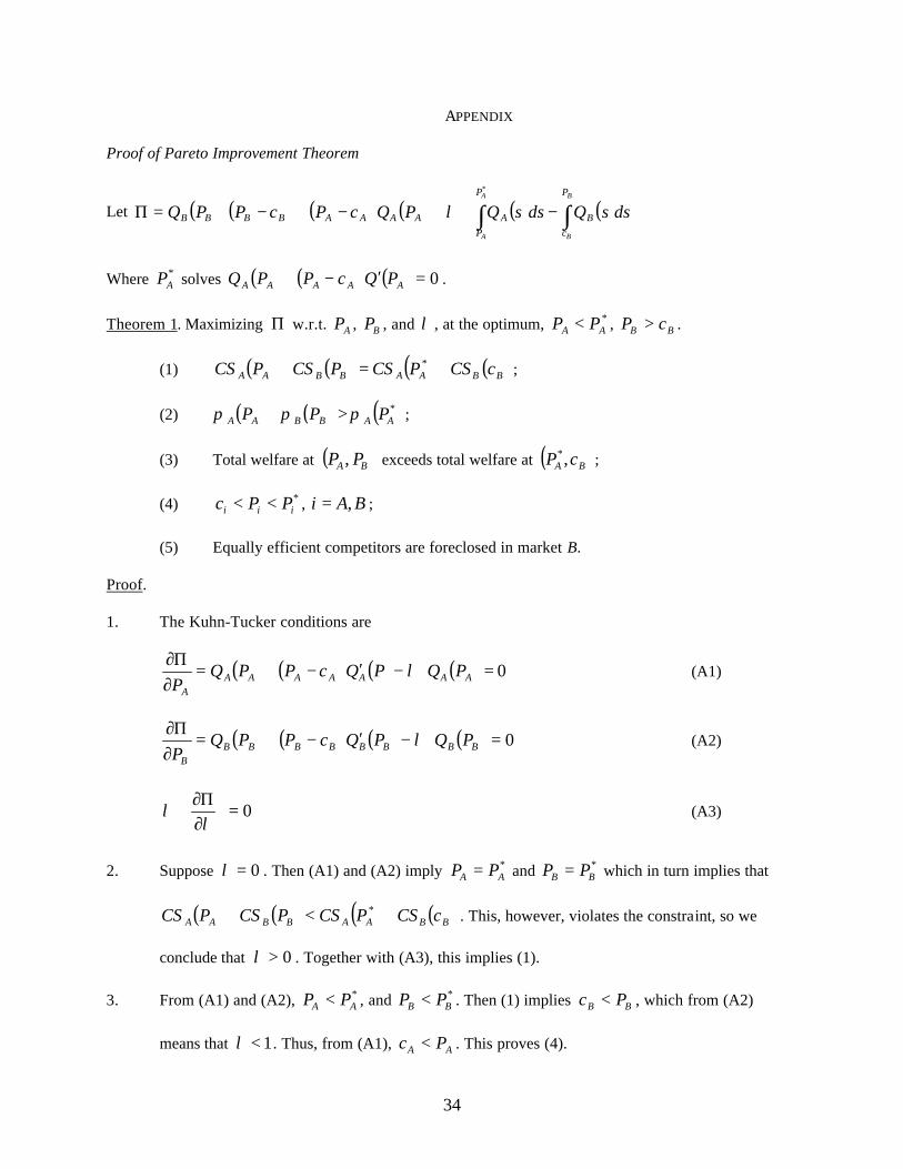
Proof of Pareto Improvement Theorem

Let ( ) ( ) ( ) ( ) ( ) ( )

−⋅+−+−⋅=Π ∫∫B

B

A

A

P

cB

P

PAAAAABBBB dssQdssQPQcPcPPQ

*

λ

Where *AP solves ( ) ( ) ( ) 0 =′−+ AAAAA PQcPPQ .

Theorem 1. Maximizing Π w.r.t. AP , BP , and λ , at the optimum, *AA PP < , BB cP > .

(1) ( ) ( ) ( ) ( )BBAABBAA cCSPCSPCSPCS +=+ * ;

(2) ( ) ( ) ( )*AABBAA PPP πππ >+ ;

(3) Total welfare at ( )BA PP , exceeds total welfare at ( )BA cP ,* ;

(4) *iii PPc << , BAi ,= ;

(5) Equally efficient competitors are foreclosed in market B.

Proof.

1. The Kuhn-Tucker conditions are

( ) ( ) ( ) ( ) 0 =⋅−′−+=∂

Π∂AAAAAAA

A

PQPQcPPQP

λ (A1)

( ) ( ) ( ) ( ) 0 =⋅−′−+=∂

Π∂BBBBBBBB

B

PQPQcPPQP

λ (A2)

0=

∂Π∂

⋅λ

λ (A3)

2. Suppose 0=λ . Then (A1) and (A2) imply *AA PP = and *

BB PP = which in turn implies that

( ) ( ) ( ) ( )BBAABBAA cCSPCSPCSPCS +<+ * . This, however, violates the constraint, so we

conclude that 0>λ . Together with (A3), this implies (1).

3. From (A1) and (A2), *AA PP < , and *

BB PP < . Then (1) implies BB Pc < , which from (A2)

means that 1<λ . Thus, from (A1), AA Pc < . This proves (4).

35

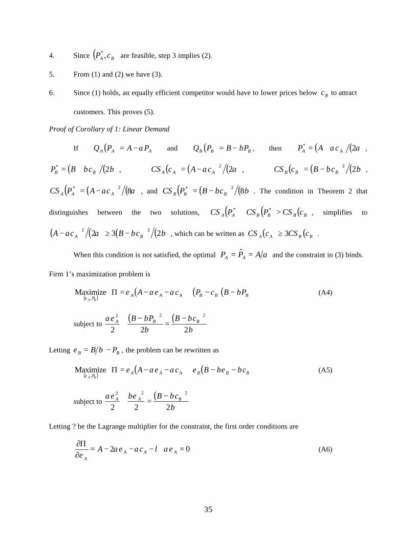
4. Since ( )BA cP ,* are feasible, step 3 implies (2).

5. From (1) and (2) we have (3).

6. Since (1) holds, an equally efficient competitor would have to lower prices below Bc to attract

customers. This proves (5).

Proof of Corollary of 1: Linear Demand

If ( ) AAA PAPQ α−= and ( ) BBB PBPQ β−= , then ( ) ( )αα 2*AA cAP += ,

( ) ( )ββ 2*BB cBP += , ( ) ( ) ( )αα 22

AAA cAcCS −= , ( ) ( ) ( )ββ 22BBB cBcCS −= ,

( ) ( ) ( )αα 82*AAA cAPCS −= , and ( ) ( ) ( )ββ 82*

BBB cBPCS −= . The condition in Theorem 2 that

distinguishes between the two solutions, ( ) ( ) ( )BBBBAA cCSPCSPCS >+ ** , simplifies to

( ) ( ) ( ) ( )ββαα 232 22BA cBcA −≥− , which can be written as ( ) ( )BBAA cCScCS 3≥ .

When this condition is not satisfied, the optimal αAPP AA == ˆ and the constraint in (3) binds.

Firm 1’s maximization problem is

{ }BA P,Maximize

ε ( ) ( )( )BBBAAA PBcPcA βααεε −−+−−=Π (A4)

subject to ( ) ( )

ββ

ββαε

222

222BBA cBPB −

=−

+

Letting BB PB −= βε , the problem can be rewritten as

{ }BA P,Maximize

ε ( ) ( )BBBAAA cBcA ββεεααεε −−+−−=Π (A5)

subject to ( )

βββεαε

222

222BAA cB −

=+

Letting ? be the Lagrange multiplier for the constraint, the first order conditions are

02 =⋅−−−=∂

Π∂AAA

A

cA αελααεε

(A6)

36

02 =⋅−−−=∂

Π∂BBB

B

cB βελββεε

, (A7)

and the solution is

( )( )

( ) ( )222AB

BAA

cAcB

cBcA

ααββα

βαε

−+−

−−= and

( )( ) ( )222

2

AB

BB

cAcB

cB

ααββαβ

βαε

−+−

−= .

The deadweight loss at the optimal loyalty discount ( )BAAA PPP ,, ε− can be written as

( ) ( ) ( ) ( )βββεαααε 22 22BBAA cBcA −−+−− , while the deadweight loss under independent

pricing ( )BA cP ,* is ( ) ( )αα 82AcA − . Thus total surplus rises after firm 1 implements loyalty pricing

whenever

( ) ( ) ( )αα

βββε

αααε

822

222ABBAA cAcBcA −

=−−

+−−

. (A8)

Substituting the optimal values for Aε and Bε and simplifying, total surplus rises whenever

( ) ( )2 2

16 9A BA c B cα β

α β− −

< , (A9)

which can be written as ( ) ( ) 916 BBAA cCScCS < .

Proof of Theorem 3

1. 1π can be written as

( ) ( ) ( ){ }

( ) ( ) 111

1

)()()(2

)(1)(

πεθ

εεθπ

+−−−+

−−+−−−=

AAAAABB

AAAAABAAAAAAAB

PvPvPqcPk

PqcPtPqcPt (A10)

where ( ) ( ) ( ) ( )1 21 1 1

12 2

B BB B

v P v PP c q P

kπ

− = − ⋅ +

is firm 1’s profit function in the B market prior to

bundling.

From these expressions, it follows that *A A A AP P Pε− = = and *

21 PPP == are feasible in the

bundling problem. Hence, no bundled discount is a possible outcome.

37

2. Differentiating with respect to 1P ,

( )( ) ( ) ( ) ( ) ( )

( ) ( )( ) ( ) ( ) ( )( )( )

*1 2

*1 2

11

1

11 1 1

1

2

2

BA A A A A A A A A A

P P P

A A A A A B B B

P P P

v PP c q P P c q P

P k

v P v P P c q P q Pk P

πθ ε ε

θ πε

= =

= =

′∂= − − − − − ∂

∂′+ ⋅ − − ⋅ − + +∂

(A11)

The last term is equal to zero at *21 PPP == , so

( )

( ) ( ) ( ) ( ) ( )

( ) ( )( ) ( ) ( ) ( )( )

*1 2

*

1

1

* * *

2

2

BA A A A A A A A A A

P P P

A A A A A B B B

v PP c q P P c q P

P k

v P v P P c q P q Pk

θπε ε

θε

= =

′∂= − − − − − ∂

′+ ⋅ − − ⋅ − +

(A12)

Since 0<′Bv and *AA PP < , the first right-hand side term is positive. Similarly, ( ) ( )A A A A Av P v Pε− >

and ( ) ( ) ( ) 0 *** >+′− PqPqcP BBB . Hence,

( )0

*21 1

1 >∂∂

== PPPPπ

. (A13)

Although the no-bundling prices are feasible for each firm, they do not satisfy the first-order conditions

for firm 1 (or firm 2). This demonstrates that a no-bundling set of prices cannot be a Nash equilibrium of

Model 2. This proves part (1) of the Theorem.

3. Denote ( ) ( )AAAA PqcP − by ( )AA Pπ . The first order conditions for AP and A AP ε− are:

( ) ( ) ( ) ( ) ( ) ( ) ( )1 112

A AAB A A B B A A A A A

v Pt P P c q P P P

kθ

θ π π ε π′

′− = − + − − (A14)

( ) ( ) ( ) ( ) ( ) ( )12 A A A

AB A A A A A A A A B B B

v Pt P P P P c q P

kε θ

θ π ε π π ε′ −

′ − = − − − − (A15)

Note that the terms inside the brackets on the right-hand sides of (A14) and (A15) have opposite sign.

Recall also that ( ) 0A Av P′ < for ˆA AP P< and ( ) 0A Av P′ = for ˆ

A AP P= . For bundling to be incentive-

38

compatible, 0Aε > must hold. From (A14) and (A15), this requires that ( ) 0A APπ ′ < and

( ) 0A A APπ ε′ − > , because these terms cannot have the same sign. Thus, *A A A AP P Pε− < < . Moreover,

( )

1

ˆ

0 A A

A P PPπ

=

∂ <∂

, so that ˆA AP P< , which completes the proof of part (2).

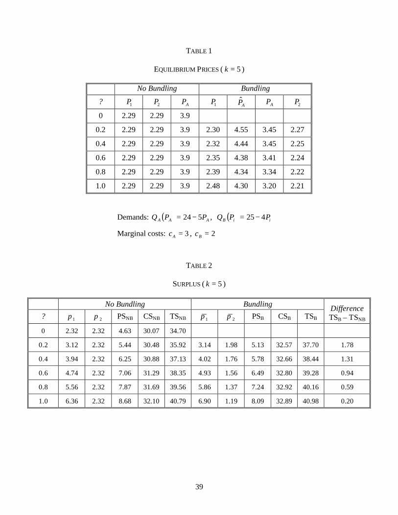
39

TABLE 1

EQUILIBRIUM PRICES ( 5k = )

No Bundling Bundling

? 1P 2P AP 1P AP AP 2P

0 2.29 2.29 3.9

0.2 2.29 2.29 3.9 2.30 4.55 3.45 2.27

0.4 2.29 2.29 3.9 2.32 4.44 3.45 2.25

0.6 2.29 2.29 3.9 2.35 4.38 3.41 2.24

0.8 2.29 2.29 3.9 2.39 4.34 3.34 2.22

1.0 2.29 2.29 3.9 2.48 4.30 3.20 2.21

Demands: ( ) AAA PPQ 524 −= , ( ) iiB PPQ 425 −=

Marginal costs: 3=Ac , 2=Bc

TABLE 2

SURPLUS ( 5k = )

No Bundling Bundling

? 1π 2π PSNB CSNB TSNB 1π 2π PSB CSB TSB Difference TSB – TSNB

0 2.32 2.32 4.63 30.07 34.70

0.2 3.12 2.32 5.44 30.48 35.92 3.14 1.98 5.13 32.57 37.70 1.78

0.4 3.94 2.32 6.25 30.88 37.13 4.02 1.76 5.78 32.66 38.44 1.31

0.6 4.74 2.32 7.06 31.29 38.35 4.93 1.56 6.49 32.80 39.28 0.94

0.8 5.56 2.32 7.87 31.69 39.56 5.86 1.37 7.24 32.92 40.16 0.59

1.0 6.36 2.32 8.68 32.10 40.79 6.90 1.19 8.09 32.89 40.98 0.20

40

TABLE 3

EQUILIBRIUM PRICES ( 5.0=θ )

No Bundling Bundling k *

1P *2P *

AP 1P AP AP 2P

5 2.29 2.29 3.9 2.33 4.41 3.435 2.25

6 2.35 2.35 3.9 2.40 4.33 3.431 2.31

7 2.41 2.41 3.9 2.45 4.29 3.432 2.37

TABLE 4

SURPLUS ( 5.0=θ )

No Bundling Bundling k 1π 2π PSNB CSNB TSNB 1π 2π PSB CSB TSB

Difference TSB – TSNB

5 4.34 2.32 6.66 31.08 37.74 4.47 1.65 6.12 32.74 38.86 1.12

6 4.77 2.74 7.51 30.40 37.91 4.92 2.15 7.08 30.67 37.75 -0.17

7 5.16 3.13 8.29 29.79 38.08 5.30 2.57 7.87 28.86 36.74 -1.34

41

BIBLIOGRAPHY

Ahlborn C, Bailey D. Discounts, rebates and selective pricing by dominant firms: a trans-Atlantic

comparison. European Competition Journal 2006;2; 101-143.

Antitrust Modernization Commission. Exclusionary conduct: refusals to deal and bundling and

loyalty discounts. Hearings September 29, 2005,

http://www.amc.gov/commission_hearings/exclusionary_conduct.htm

Brennan, TJ. Competition as an entry barrier? consumer and total welfare benefits of bundling,

AEI-Brookings Joint Center for Regulatory Studies Related Publication 2005 05-08.

Brown SJ, Sibley DS. The theory of public utility pricing. Cambridge University Press:

Cambridge; 1986.

Burstein ML. The economics of tie-in sales. Review of Economics and Statistics 1960;42; 68-73.

Carlton D. A general analysis of exclusionary conduct and refusals to deal—why Aspen and

Kodak are misguided. Antitrust Law Journal 2001;68; 659-683.

Carlton D, Waldman M. The strategic use of tying to preserve and create market power in

evolving industries. RAND Journal of Economics 2002;33; 194-220.

European Commission. DG Competition discussion paper on the application of Article 82 of the

Treaty to exclusionary abuses. 2005

http://ec.europa.eu/comm/competition/antitrust/others/discpaper2005.pdf

Greenlee P, Reitman, D. Competing with loyalty discounts. EAG Discussion Paper 04-02.

Washington, DC: U.S. Department of Justice, 2004.

Greenlee P, Reitman D. Distinguishing competitive and exclusionary uses of loyalty discounts.

Antitrust Bulletin 2005;50; 441-464.

Hensley S. Scaled up: biggest drug firm faces generics but has an edge: its very bigness. Wall

Street Journal August 23, 2004, A1.

Iyer G, Villas-Boas JM. A bargaining theory of distribution channels. Journal of Marketing

Research 2003;40; 80-100.

Kadiyali V, Chintagunta P, Vilcassim N. Manufacturer-retailer channel interactions and

implications for channel power: An empirical investigation of pricing in a local market.

Marketing Science 2000;19; 127-148.

Kobayashi BH. The economics of loyalty discounts and antitrust law in the United States.

Competition Policy International 2005;1; 115-148.

Kolay S, Shaffer G, Ordover JA. All-units discounts in retail contracts. Journal of Economics &

Management Strategy 2004;13; 429-459.

42

Mathewson F, Winter R. Tying as a response to demand uncertainty. RAND Journal of

Economics 1997;28; 566-583.

Nalebuff B. Bundling as an entry barrier. Quarterly Journal of Economics 2004a;119; 159-187.

Nalebuff B. Bundling as a way to leverage monopoly. Yale SOM Working Paper 2004b; ES-36.

Nalebuff B. Exclusionary bundling. Antitrust Bulletin 2005;50; 321-370.

Ordover JA. Willig RD. An economic definition of predation: pricing and product innovation.

Yale Law Journal 1981;91; 8-53.

Parloff R. Intel’s worst nightmare. Fortune August 21, 2006, 60.

Pollack A. Johnson sues Amgen over sales practice. New York Times October 13, 2005, C2.

Rubinfeld DL. 3M’s Bundling rebates: an economic perspective. University of Chicago Law

Review 2005;72; 243-264.

Sibley DS, Srinagesh P. Multiproduct nonlinear pricing with multiple taste characteristics. RAND

Journal of Economics 1997;28; 684-707.

Tom WK, Balto DA, Averitt NW. Anticompetitive aspects of market-share discounts and other

incentives to exclusive dealing. Antitrust Law Journal 2000;67; 615-639.

Whinston MD. Tying, foreclosure and exclusion. American Economic Review 1990;80; 837-859.