An Analysis Pathway for the QuantitativeEvaluation of Public Transport Systems

Stephen Gilmore1, Mirco Tribastone2, and Andrea Vandin2

1 Laboratory for Foundations of Computer Science, University of Edinburgh2 Electronics and Computer Science, University of Southampton

Abstract. We consider the problem of establishing quantitative service-level agreements in public services such as transportation systems. Wedescribe the integration of quantitative analysis tools for data fitting,model generation, simulation, and statistical model-checking, creating ananalysis pathway leading from system measurement data to verificationresults. We apply our pathway to the problem of determining whetherpublic bus systems are delivering an appropriate quality of service asrequired by regulators. We exercise the pathway on service data obtainedfrom Lothian Buses about the arrival and departure times of their buseson key bus routes through the city of Edinburgh. Although we includeonly that example in the present paper, our methods are sufficientlygeneral to apply to other transport systems and other cities.

1 Introduction

Modern public transport systems are richly instrumented. The vehicles in amodern bus fleet are equipped with accurate GPS receivers, Wi-Fi, and on-board communications, allowing them to report their location for purposes suchas fleet management and arrival-time prediction. High-frequency, high-resolutionlocation data streams back from the vehicles in the fleet to be consumed by thepredictive models used in real-time bus tracking systems.

We live in a data-hungry world. Users of public transport systems now expectto be able to access live data about arrival times, transit connections, servicedisruptions, and many other types of status updates and reports at almost everystage of their journey. Studies suggest that providing real-time information onbus journeys and arrival times in this way encourages greater use of buses [1] withbeneficial effects for the bus service. In contrast, when use of buses decreases,transport experts suggest that this aggravates existing problems such as out-dated routes, bunching of vehicles, and insufficient provision of greenways or buspriority lanes. Each of these problems makes operating the bus service more dif-ficult. Bus timetables become less dependable, new passengers are discouragedfrom using the bus service due to bad publicity, which leads inevitably to budgetcuts that further accelerate the decline of the service.

Service regulators are no less data-hungry than passengers, requiring trans-port operators to report service-level statistics and key performance indica-tors which are used to assess the service delivered in practice against regula-tory requirements on the quality of service expected. Many of these regulatory

requirements relate to punctuality of buses, defined in terms of the percentageof buses which depart within the window of tolerance around the timetableddeparture time; and reliability of buses, defined in terms of the number of milesplanned and the number of miles operated. The terms schedule adherence oron-time performance are also used to refer to the degree of success of a trans-portation service running to the published timetable.

With the aim of helping service providers to be able to work with modelswhich can be used to analyse and predict on-time performance, we have con-nected a set of modelling and analysis tools into an analysis pathway, startingfrom system measurement data, going through data fitting, model generation,simulation and statistical model-checking to compute verification results whichare of significance both to service providers and to regulatory authorities.

The steps of the analysis pathway, depicted in Figure 1, are as follows:

1. Data is harvested from a bus tracking system to compile an empirical cumu-lative distribution function data set of recorded journey times for each stageof the bus journey. In this paper, we generate inputs to the system usingthe BusTracker automatic vehicle tracking system developed by the City ofEdinburgh council and Lothian Buses [2].

2. The software tool HyperStar [3] is used to fit phase-type distributions to thedata sets.

3. A phase-type distribution enables a Markovian representation of journeytimes which can be encoded in high-level formalisms such as stochasticprocess algebras. In particular, we use the Bus Kernel model generator(BusKer), a Java application which consumes the phase-type distributionparameters computed by HyperStar and generates a formal model of thebus journey expressed in the Bio-PEPA stochastic process algebra [4]. Inaddition, BusKer generates an expression in MultiQuaTEx, the query lan-guage supported by the MultiVeStA statistical model-checker [5]. This isused to formally express queries on service-level agreements about the busroute under study.

4. The Bio-PEPA Eclipse Plugin [6] is used to perform stochastic simulationsof the Bio-PEPA model.

5. MultiVeStA is hooked to the simulation engine of the Bio-PEPA EclipsePlugin, consuming individual simulation events to evaluate the automaticallygenerated MultiQuaTEx expressions. It produces as its results plots of therelated quantitative properties.

We are devoting more than the usual amount of effort to ensuring that ourtools are user-friendly and easy-to-use. This is because we want our softwaretools to be used “in-house” by service providers because only then can serviceproviders retain control over access to their own proprietary data about theirservice provision. With respect to ease-of-use in particular, making model param-eterisation simpler is a crucial step in making models re-usable. Because vehicleoccupancy fluctuates according to the seasons, with the consequence that busesspend more or less time at bus stops boarding passengers, it is essential to be

BusTracker HyperStar BusKer Bio-PEPA MultiVeStA

Fig. 1. The analysis pathway.

able to re-parameterise and re-run models for different data sets from differentmonths of the year.

It is also necessary to be able to re-run an analysis based on historical mea-surement data if timetables change, or the key definitions used in the evaluationof regulatory requirements change. Evidently, a high degree of automation in theprocess is essential, hence our interest in an analysis pathway.

Related work. We are not aware of other toolchains based on formal methodsfor the quantitative analysis of public transportation systems. The same bussystem is studied in [7], from which we inherited the data-set acquisition andits fitting to phase-type distributions. Differently from our approach, in [7] dif-ferent software tools are individually used to perform distinct analyses of thescenario. For example, the Traviando [8] post-mortem simulation trace anal-yser is fed with precomputed simulation traces of a Bio-PEPA model similarto ours, and the probabilistic model checker PRISM [9] is used to analyse acorresponding model defined in the PRISM’s input language. More in general,our approach takes inspiration from generative programming techniques [10], inthat we aim at automatic generation of possibly large stochastic process algebramodels (our target language) from more compact higher-level descriptions (i.e.,the timetable representation and the model parameters). The generation of Mul-tiQuaTEx expressions fits well with the literature on higher-level specificationpatterns for temporal logic formulae [11]: temporal logics are not widespreadin industry, as they require a high degree mathematical maturity. Furthermore,most system requirements are written in natural language, and often containambiguities which make it difficult to accurately formalise them. In an attemptto ease the use of temporal logic, [11] gives a pattern-based classification forcapturing requirements, paving the way for semi-automated methodologies forthe generation of inputs to model checking tools. From a general perspective, inthis work we fix the property patterns of interest, and completely hide propertygeneration and evaluation to the end user.

Paper structure. Section 2 describes the analysis problem in greater detail andpresents the key definitions used in the paper. Section 3 describes the softwaretools in the analysis pathway. Section 4 presents the software analyser which

combines these disparate tools. Section 5 presents our analysis in terms of thekey definitions of the paper. Conclusions are presented in Section 6.

2 The analysis problem

The notion of punctuality is defined in terms of a “window of tolerance” aroundthe departure times advertised in the timetable. Perhaps not very surprisingly,this notion differs between different operators and different countries, for instance:

– According to Transport for London, a bus is considered to be on time if itdeparts between two minutes and 30 seconds early and five minutes late [12].

– In England outside London, a bus is considered to be on time if it departsbetween one minute early and five minutes, 59 seconds late [13].

– In Scotland, according to the definitions reported in the Scottish Govern-ment’s Bus Punctuality Improvement Partnerships report, a bus is consid-ered to be on time if it departs between one minute early and five minuteslate [14].

Each region has a definition of on-time in terms of the window of tolerance butclearly when comparing the quality of service in one region with the quality ofservice in another it is necessary to be able to re-evaluate the service deliveredhistorically against the definitions used by another.

Our problem is to generate a mathematical model which allows us to analysethe following properties, for each bus stop advertised in a timetable.

P1. The average time of departure from the bus stop.P2. The average distance of the departure time from the timetabled time.P3. The probability that a bus departs on time.P4. The probability of an early departure.P5. The probability of a late departure.

Let us remark that since the window of tolerance is asymmetric with respectto the timetable, property P2 is formally defined as the expected value of theabsolute value of the difference between the time of departure and the respectivetimetabled time. Let us also notice that properties P3–P5 clearly depend on thenotion of punctuality adopted.

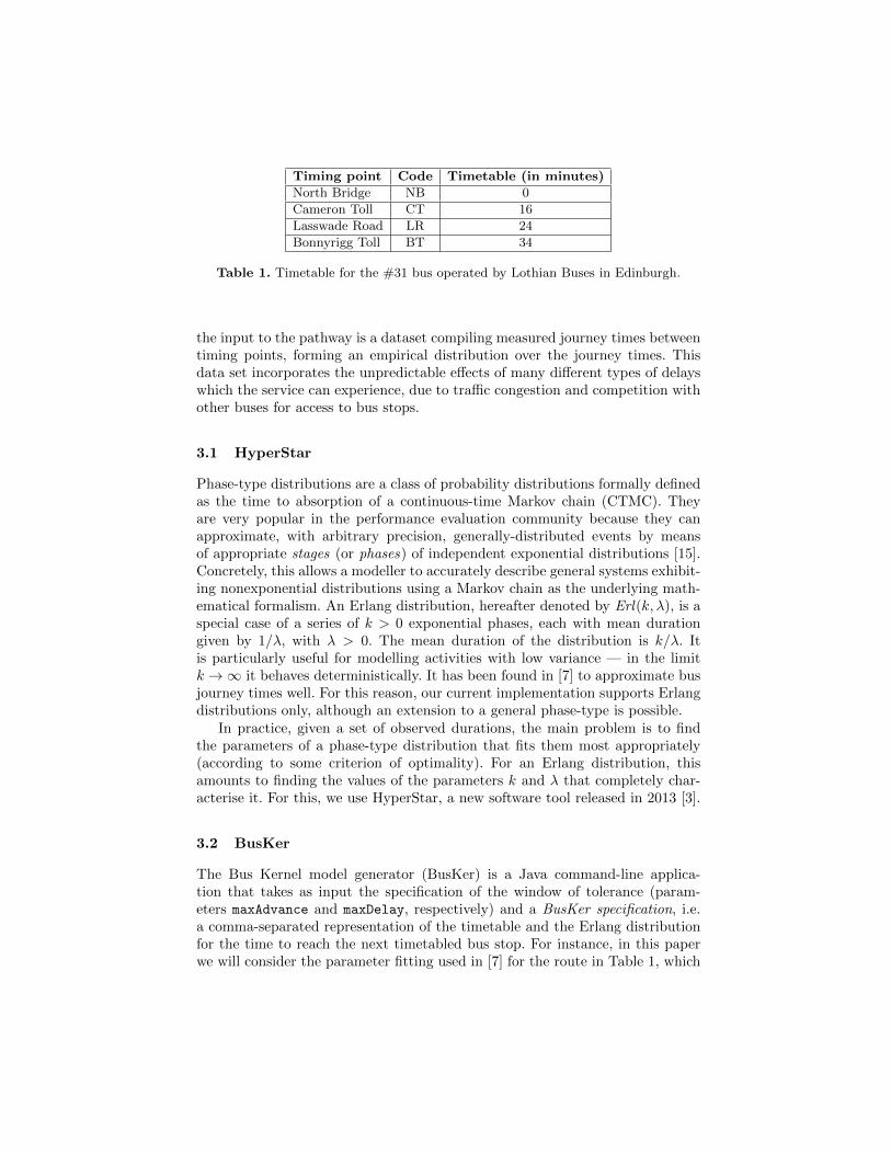
To be more concrete, in this paper we focus on a particular bus route. Specif-ically, we consider the Lothian Buses #31 bus on its journey from North Bridgein Edinburgh’s city centre to Bonnyrigg Toll in the south, passing through theCameron Toll and Lasswade Road timing points. The same bus route has beenstudied in [7], as discussed in Section 1. Table 1 shows its timetable, where thedeparture time from North Bridge is taken as the reference time 0.

3 The analysis pathway

In this section we describe in more detail the modelling tools and formal lan-guages of our analysis pathway, as well as their integration. The raw data which is

Timing point Code Timetable (in minutes)

North Bridge NB 0

Cameron Toll CT 16

Lasswade Road LR 24

Bonnyrigg Toll BT 34

Table 1. Timetable for the #31 bus operated by Lothian Buses in Edinburgh.

the input to the pathway is a dataset compiling measured journey times betweentiming points, forming an empirical distribution over the journey times. Thisdata set incorporates the unpredictable effects of many different types of delayswhich the service can experience, due to traffic congestion and competition withother buses for access to bus stops.

3.1 HyperStar

Phase-type distributions are a class of probability distributions formally definedas the time to absorption of a continuous-time Markov chain (CTMC). Theyare very popular in the performance evaluation community because they canapproximate, with arbitrary precision, generally-distributed events by meansof appropriate stages (or phases) of independent exponential distributions [15].Concretely, this allows a modeller to accurately describe general systems exhibit-ing nonexponential distributions using a Markov chain as the underlying math-ematical formalism. An Erlang distribution, hereafter denoted by Erl(k, λ), is aspecial case of a series of k > 0 exponential phases, each with mean durationgiven by 1/λ, with λ > 0. The mean duration of the distribution is k/λ. Itis particularly useful for modelling activities with low variance — in the limitk →∞ it behaves deterministically. It has been found in [7] to approximate busjourney times well. For this reason, our current implementation supports Erlangdistributions only, although an extension to a general phase-type is possible.

In practice, given a set of observed durations, the main problem is to findthe parameters of a phase-type distribution that fits them most appropriately(according to some criterion of optimality). For an Erlang distribution, thisamounts to finding the values of the parameters k and λ that completely char-acterise it. For this, we use HyperStar, a new software tool released in 2013 [3].

3.2 BusKer

The Bus Kernel model generator (BusKer) is a Java command-line applica-tion that takes as input the specification of the window of tolerance (param-eters maxAdvance and maxDelay, respectively) and a BusKer specification, i.e.a comma-separated representation of the timetable and the Erlang distributionfor the time to reach the next timetabled bus stop. For instance, in this paperwe will consider the parameter fitting used in [7] for the route in Table 1, which

yields the following BusKer specification:

# Timing point ,Code,Timetable, k, λ

North Bridge, NB, 0, 105, 6.47

Cameron Toll, CT, 16, 83, 8.79 (1)

Lasswade Road, LR, 24, 98, 10.54

Bonnyrigg Toll, BT, 34,−,−

As a result, BusKer generates the inputs for the next two steps of our analysispathway: a Bio-PEPA model of the bus service, and the MultiQuaTEx expressionanalysed by MultiVeStA to state the quality of the studied bus service withrespect to the provided window of tolerance.

3.3 Bio-PEPA

Although designed for application to modelling problems in biological systems,Bio-PEPA has been effectively applied to problems as diverse as crowd dynam-ics [16], emergency egress [17] and swarm robotics [18]. Here, we use it becauseit is a stochastic process algebra with an underlying CTMC semantics; as suchit is possible to encode phase-type distributions in Bio-PEPA. Furthermore, itis implemented by a software tool, the BioPEPA Eclipse Plugin, which supportsstochastic simulation in a way that is easily consumable by MultiVeStA. Refer-ring the reader to [4] for the complete formal account, we will use the followingsimplified BusKer specification to briefly overview the language:

# Timing point ,Code,Timetable, k, λ

North Bridge, NB, 0, 3, 0.19 (2)

Cameron Toll, CT, 16,−,−

BusKer will generate the specification shown in Listing 1.1. The model concernsthe five species NB 1, NB 2, NB 3, CT 1 and DepsFromNB, representing the numberof buses in North Bridge (NB 1), those in the first (NB 2) and second (NB 3) partof the journey from North Bridge to Cameron Toll, and the number of buses atCameron Toll (CT 1). Finally, DepsFromNB is an observer process used to countthe number of departures from North Bridge. Lines 16–18 provide the initialsystem configuration: one bus is in North Bridge, while all the other populationsare set to 0. A reaction prefix such as NBtoCT 1<< in a species definition (e.g.NB 1 = NBtoCT 1<< at line 8) causes the population count of that species (NB 1)to decrease by one when the reaction NBtoCT 1 occurs. In particular, line 3specifies that the reaction NBtoCT 1 occurs with a rate obtained by multiplyingthe constant 0.19 with the population count of the species NB 1. In our modelwe follow the journey of a single prototypical bus, so this product in the rateexpression acts as a switch, allowing the reaction to fire when a bus is presentand preventing it from firing at other times (because the rate evaluates to 0when a bus is not present). Similar to this is the case of the reaction prefix

1 // Definitions of rate functions2 // Functions for North Bridge -> Cameron Toll (3 phases)3 NBtoCT_1 = [0.19 * NB_1];4 NBtoCT_2 = [0.19 * NB_2];5 NBtoCT_ARRIVED = [0.19 * NB_3];6 // Definitions of processes7 // Processes for North Bridge -> Cameron Toll (3 phases)8 NB_1 = NBtoCT_1 << ;9 NB_2 = NBtoCT_1 >> + NBtoCT_2 << ;

10 NB_3 = NBtoCT_2 >> + NBtoCT_ARRIVED << ;11 // Cameron Toll is the final stop.12 CT_1 = NBtoCT_ARRIVED >> ;13 // State observations14 DepsFromNB = NBtoCT_1 >> ;15 // Initial configuration of the system (one bus in North Bridge)16 NB_1 [1] <*> NB_2 [0] <*> NB_3 [0] <*>17 CT_1 [0] <*>18 DepsFromNB [0]

Listing 1.1. The Bio-PEPA model generated by BusKer for the scenario of (2)

NBtoCT 1>>, the only difference being that in this case the involved populationcounts increase by one. For example, line 14 specifies that the population of thespecies DepsFromNB increases by one whenever the reaction NBtoCT 1 occurs,making DepsFromNB a de facto counter for the departures of buses from NorthBridge. In contrast, line 10 specifies that the population of the species NB 3, i.e.the buses in the second part of the journey from North Bridge to Cameron Toll,increases by one whenever a bus moves from the first to the second part of thejourney (NBtoCT 2>>), and decreases by one whenever a bus arrives at CameronToll (NBtoCT ARRIVED<<).

The Bio-PEPA model built from the input to BusKer is a statistically-plausible stochastic model of the journey of a prototypical bus travelling fromthe first to the last specified bus stops, using the Erlang parameters learnt fromthe measurement data which has been processed by HyperStar. Clearly, the pre-dictive power of this model depends crucially on the quality and scope of thedata supplied to HyperStar. Because it is ultimately learnt from data, the modelwill incorporate the effects of contention for bus stops with other buses servingthe same route, and, for good or ill, it will incorporate the influence of any atyp-ical events (e.g. unusually long delays) which occurred during the measurementperiod.

3.4 MultiVeStA

MultiVeStA [5] is a recently-developed Java-based distributed statistical modelchecker which allows its users to enrich existing discrete event simulators withautomated and statistical analysis capabilities. The analysis algorithms of Mul-tiVeStA do not depend on the underlying simulation engine: MultiVeStA onlymakes the assumption that multiple discrete event simulations can be performedon the input model. The tool has been used to reason about collision-avoidancerobots [19], volunteer clouds [20] and crowd-steering [21] scenarios.

1 DepartureTime(depsFromBusStop) =2 i f { s.rval(depsFromBusStop) == 1.0 } then s.rval("time")3 else # DepartureTime(depsFromBusStop)4 f i ;5 eval E[ DepartureTime (" DepsFromNB ") ]; eval E[ DepartureTime (" DepsFromCT ") ];6 eval E[ DepartureTime (" DepsFromLR ") ];

Listing 1.2. A MultiQuaTEx expression to query expected departure times

MultiVeStA comes with a property specification language, MultiQuaTEx,which makes it possible for users to express and evaluate many properties overthe same simulated path. In contrast to Continuous Stochastic Logic [22, 23]and Probabilistic Computation Tree Logic [24] commonly used in probabilisticand statistical model checking, MultiQuaTEx allows users to define their ownparametric recursive temporal operators within the logic itself, and to queryreal-typed properties, rather than just probabilities. In particular, with Multi-QuaTEx we can express all the properties listed in Section 2.

A MultiQuaTEx expression is evaluated statistically. Given a statistical esti-mate x, then with probability (1 − α) its true value lies within the interval[x − δ/2, x + δ/2], where (α, δ) is a user-specified confidence interval. An in-depth presentation of MultiQuaTEx is out of the scope of this paper, but canbe found in [5].

Listing 1.2 provides a MultiQuaTEx expression to estimate the expecteddeparture times from each bus stop of interest (property P1) using the BusKerspecification (1). Lines 5–6 specify the three expected values to be estimated,i.e. the departure times from North Bridge, Cameron Toll and Lasswade Road.Lines 1–4 specify a parametric recursive temporal operator which returns, foreach simulation, the departure time of the bus from the bus stop specified asthe parameter. This is iteratively evaluated by performing steps of simulations(triggered by the operator #) until the guard of the if statement is satisfied,i.e. until a departure occurs from the selected bus stop. Intuitively, as discussedin Section 3.3, the Bio-PEPA model generated by BusKer counts the depar-tures from each bus stop by defining observer processes DepsFromNB, DepsFromCTand DepsFromLR whose populations are incremented every time the correspond-ing event happens. Finally, we note that MultiVeStA can access informationabout the current state of the simulation with s.rval(observation), whereobservation can be the current simulated time (i.e. time), or the current pop-ulation of a species (e.g. "DepsFromNB").

4 Tool chaining: The Bus Analyzer

The last three tools of our analysis pathway, highlighted in Figure 1, have beenintegrated in a single tool called TBA: The Bus Analyzer. TBA hides from theuser the steps involved in the generation of the Bio-PEPA model and of theMultiQuaTEx expression, as well as the invocation of MultiVeStA. TBA can be

Fig. 2. Plot generated by TBA for the specification presented in Equation (1), and the(1,5) window of tolerance.

downloaded, together with our BusKer specification (1), from the Tools sectionof the QUANTICOL web-site at http://www.quanticol.eu/.

A first clear advantage brought by TBA is the automation of the analysisphase, as the user only has to execute the command

java -jar TBA.jar busker scenario.busker maxAdv maxDelay [servers] (3)

where scenario.busker is a file containing a BusKer specification, and max-Adv and maxDelay specify the required window of tolerance (in minutes). Theoptional parameter servers gives the degree of parallelism to automatically dis-tribute independent simulations across CPU cores.

TBA evaluates properties P1–P5. The results are provided to the user via aGUI consisting of an interactive scatter plot containing a point for each studiedproperty, and are also stored on disk. For example, the interactive plot allowsthe modeller to hide some properties, to apply zooming or rescaling operations,to change the considered boundaries, and to save the plot as a picture. Figure 2depicts the plot obtained for the BusKer specification (1) when considering theScottish window of tolerance, i.e., maxAdv=1 and maxDelay=5. A discussion of

1 // Definitions of rate functions2 // Functions for North Bridge -> Cameron Toll (105 phases)3 NBtoCT_1 = [6.47 * NB_1];4 ...5 NBtoCT_104 = [6.47 * NB_104 ];6 NBtoCT_ARRIVED = [6.47 * NB_105 ];7 // Functions for Cameron Toll -> Lasswade Road (83 phases)8 CTtoLR_1 = [8.79 * CT_1];9 ...

10 CTtoLR_82 = [8.79 * CT_82];11 CTtoLR_ARRIVED = [8.79 * CT_83];12 // Functions for Lasswade Road -> Bonnyrigg Toll (98 phases)13 LRtoBT_1 = [10.54 * LR_1];14 ...15 LRtoBT_97 = [10.54 * LR_97];16 LRtoBT_ARRIVED = [10.54 * LR_98 ];17 // Definitions of processes18 // Processes for North Bridge -> Cameron Toll (105 phases)19 NB_1 = NBtoCT_1 <<;20 NB_2 = NBtoCT_1 >> + NBtoCT_2 <<;21 ...22 NB_104 = NBtoCT_103 >> + NBtoCT_104 <<;23 NB_105 = NBtoCT_104 >> + NBtoCT_ARRIVED <<;24 // Processes for Cameron Toll -> Lasswade Road (83 phases)25 CT_1 = NBtoCT_ARRIVED >> + CTtoLR_1 <<;26 CT_2 = CTtoLR_1 >> + CTtoLR_2 <<;27 ...28 CT_82 = CTtoLR_81 >> + CTtoLR_82 <<;29 CT_83 = CTtoLR_82 >> + CTtoLR_ARRIVED <<;30 // Processes for Lasswade Road -> Bonnyrigg Toll (98 phases)31 LR_1 = CTtoLR_ARRIVED >> + LRtoBT_1 <<;32 LR_2 = LRtoBT_1 >> + LRtoBT_2 <<;33 ...34 LR_97 = LRtoBT_96 >> + LRtoBT_97 <<;35 LR_98 = LRtoBT_97 >> + LRtoBT_ARRIVED <<;36 // Bonnyrigg Toll is the final stop.37 BT_1 = LRtoBT_ARRIVED >>;38 // State observations39 DepsFromNB = NBtoCT_1 >>; DepsFromCT = CTtoLR_1 >>; DepsFromLR = LRtoBT_1 >>;40 // Initial configuration of the system (one bus in North Bridge)41 NB_1 [1] <*> ... <*> NB_105 [0] <*>42 CT_1 [0] <*> ... <*> CT_83 [0] <*>43 LR_1 [0] <*> ... <*> LR_98 [0] <*> BT_1 [0] <*>44 DepsFromNB [0] <*> DepsFromCT [0] <*> DepsFromLR [0]

Listing 1.3. The Bio-PEPA model generated by BusKer for input Equation (1)

the analysis is provided in Section 5. In the remainder of this section we focus onthe usability and accessibility advantages provided by chaining the three tools.

Clearly, given that TBA hides the generation of the model and of the prop-erty, as well as their analysis, the user is not required to learn the two formallanguages, nor to use their related tools. Furthermore, for realistic bus scenar-ios the generated Bio-PEPA models and MultiQuaTEx expressions tend to belarge and thus error-prone to write down manually. For example, the Bio-PEPAmodel generated by TBA for our scenario is almost 900 lines long, as sketchedin Listing 1.3. This is due to the the fact that the journeys between bus stopsare modelled using Erlang distributions with many phases, and each phase isassociated with a distinct species (hence at least a line in the source code). Morespecifically, Listing 1.3 can be divided in four parts: lines 1–16 define the rates

1 // Static part of the expression : the parametric temporal operators2 // Probabilities of departing on time , too early or too late3 DepartedOnTime(depsFromBusStop ,timeTabledDep ,maxAdv ,maxDelay) =4 i f { s.rval(depsFromBusStop) == 1.0 }5 then CheckIfDepOnTime(depsFromBusStop ,timeTabledDep ,maxAdv ,maxDelay)6 else # DepartedOnTime(depsFromBusStop ,timeTabledDep ,maxAdv ,maxDelay)7 f i ;8 CheckIfDepOnTime(depsFromBusStop ,timeTabledDep ,maxAdv ,maxDelay) =9 i f { timeTabledDep - s.rval("time") > maxAdv }

10 then 0.011 else i f { s.rval("time") - timeTabledDep > maxDelay }12 then 0.0 else 1.013 f i14 f i ;15 DepartedTooEarly(depsFromBusStop ,timeTabledDep ,maxAdv) =// like DepartedOnTime16 DepartedTooLate(depsFromBusStop ,timeTabledDep ,maxDelay)=// like DepartedOnTime17 // Expceted departure time18 DepartureTime(depsFromBusStop) = //as in Listing 1.219 // Expceted deviation from the timetabled departure time20 DistanceFromTimeTable(depsFromBusStop ,timeTabledDep) =21 i f { s.rval(depsFromBusStop) == 1.0 }22 then ComputeDistanceFromTimeTable(depsFromBusStop ,timeTabledDep)23 else # DistanceFromTimeTable(depsFromBusStop ,timeTabledDep)24 f i ;25 ComputeDistanceFromTimeTable(depsFromBusStop ,timeTabledDep) =26 i f { timeTabledDep > s.rval("time") }27 then timeTabledDep - s.rval("time") else s.rval("time") - timeTabledDep28 f i ;29 // Static part of the expression : the 15 properties to be estimated30 eval E[ DepartureTime (" DepsFromNB ") ];31 eval E[ DistanceFromTimeTable (" DepsFromNB ",0.0) ];32 eval E[ DepartedOnTime (" DepsFromNB " ,0.0 ,1.0 ,5.0) ];33 eval E[ DepartedTooEarly (" DepsFromNB " ,0.0 ,1.0) ];34 eval E[ DepartedTooLate (" DepsFromNB " ,0.0 ,5.0) ];35 // same eval clauses for " DepsFromCT ", and "16.0" rather than 0.036 // same eval clauses for " DepsFromLR ", and "24.0" rather than 0.0

Listing 1.4. The MultiQuaTEx expression generated by BusKer

with which the modelled prototypical bus moves, lines 17–36 define the processesspecifying the bus’s stochastic behaviour, lines 37–38 define the state observa-tions of interest, while lines 39–44 specify the initial configuration of the system.The third section only depends on the number of considered bus stops, while, asdepicted by the ellipsis, the other ones also depend on the number of phases ofthe provided BusKer specification.

The MultiQuaTEx expression generated by BusKer for our scenario is a fixedlength for any window of tolerance. It is sketched in Listing 1.4 for the Scottishwindow of tolerance. Overall it evaluates fifteen properties, i.e., P1–P5 for eachof the three bus stops. Lines 1–28 define the parametric recursive temporal oper-ators which specify how to compute such properties, whereas lines 29–36 list thefifteen properties to be estimated. For each simulation, each temporal operatorobserves the bus stop provided as a parameter, specifically: DepartedOnTime,DepartedTooEarly and DepartedTooLate return 1 if the bus departed on time,too early, or too late, respectively. DepartureTime returns the departure time ofthe bus, while DistanceFromTimeTable returns the absolute value of the differ-ence between the actual departure time and the timetabled one. That expression

North Bridge Cameron Toll Lasswade Road

P1 0.32 16.42 25.84

P2 0.32 1.28 2.13

P3 1.00 0.81 0.88

P4 0.00 0.19 0.04

P5 0.00 0.00 0.06

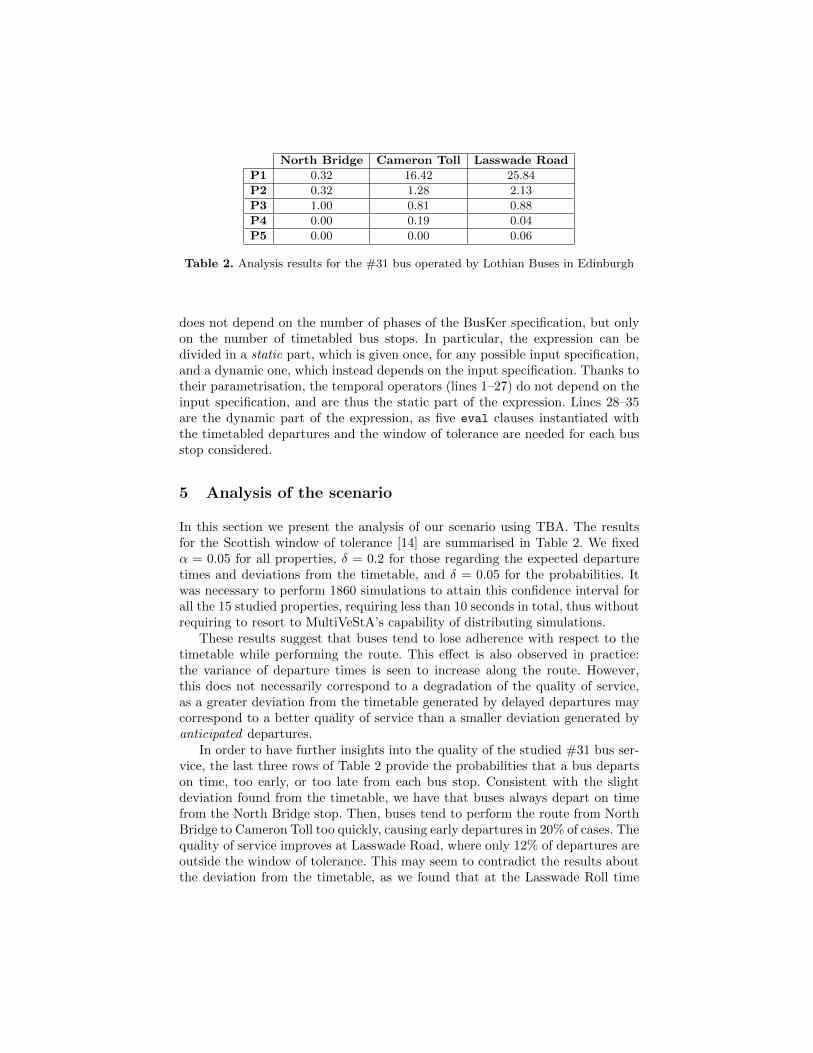
Table 2. Analysis results for the #31 bus operated by Lothian Buses in Edinburgh

does not depend on the number of phases of the BusKer specification, but onlyon the number of timetabled bus stops. In particular, the expression can bedivided in a static part, which is given once, for any possible input specification,and a dynamic one, which instead depends on the input specification. Thanks totheir parametrisation, the temporal operators (lines 1–27) do not depend on theinput specification, and are thus the static part of the expression. Lines 28–35are the dynamic part of the expression, as five eval clauses instantiated withthe timetabled departures and the window of tolerance are needed for each busstop considered.

5 Analysis of the scenario

In this section we present the analysis of our scenario using TBA. The resultsfor the Scottish window of tolerance [14] are summarised in Table 2. We fixedα = 0.05 for all properties, δ = 0.2 for those regarding the expected departuretimes and deviations from the timetable, and δ = 0.05 for the probabilities. Itwas necessary to perform 1860 simulations to attain this confidence interval forall the 15 studied properties, requiring less than 10 seconds in total, thus withoutrequiring to resort to MultiVeStA’s capability of distributing simulations.

These results suggest that buses tend to lose adherence with respect to thetimetable while performing the route. This effect is also observed in practice:the variance of departure times is seen to increase along the route. However,this does not necessarily correspond to a degradation of the quality of service,as a greater deviation from the timetable generated by delayed departures maycorrespond to a better quality of service than a smaller deviation generated byanticipated departures.

In order to have further insights into the quality of the studied #31 bus ser-vice, the last three rows of Table 2 provide the probabilities that a bus departson time, too early, or too late from each bus stop. Consistent with the slightdeviation found from the timetable, we have that buses always depart on timefrom the North Bridge stop. Then, buses tend to perform the route from NorthBridge to Cameron Toll too quickly, causing early departures in 20% of cases. Thequality of service improves at Lasswade Road, where only 12% of departures areoutside the window of tolerance. This may seem to contradict the results aboutthe deviation from the timetable, as we found that at the Lasswade Roll time

North Bridge Cameron Toll Lasswade RoadSC EN SC EN SC EN

P3 1.00 1.00 0.81 0.82 0.88 0.92

P4 0.00 0.00 0.19 0.18 0.04 0.05

P5 0.00 0.00 0.00 0.00 0.06 0.03

Table 3. The quality of the #31 bus service for the Scottish (SC) and English (EN)window of tolerance.

point there is a greater deviation from the timetable with respect to that atCameron Toll. However, this is explained by noticing that our analysis tells usthat the deviations from the timetable are mainly caused by anticipated depar-tures at Cameron Toll, and by delayed departures at Lasswade Road. In fact, wefirst of all notice that the expected departure time is 0.42 minutes greater thanthe timetabled one at Cameron Toll, and 1.84 at Lasswade Road.

Furthermore, we have early departures in 20% of cases and no late departuresat Cameron Toll. Instead, at Lasswade Road we have early departures in only 4%of cases, and late departures in 6% of cases. In conclusion, we find that buses tendto spend more time than is scheduled in performing the journey from CameronToll to Lasswade Road, thus absorbing the effect of earlier departures fromCameron Toll, leading to a halved percentage of departures there outside thewindow of tolerance with respect to Cameron Toll.

It is worthwhile to note that analysing the quality of service with respectto other windows of tolerance only requires launching the command (3) withdifferent parameters. For example, Table 3 compares the results using the Scot-tish window of tolerance (SC), and the English one (EN), the latter obtainedby setting parameters maxAdv=1 and maxDelay=5.59. Not surprisingly, the tabledepicts a slightly better quality of service for the same data when consideringthe looser English window of tolerance rather than the stricter Scottish one.

6 Conclusions

In this paper we have presented an analysis pathway for the quantitative eval-uation of service-level agreements for public transportation systems. Althoughwe discussed a concrete application focussing on a specific bus route in a spe-cific city, our approach is more general and it can be in principle applied toother transportation systems publishing timetabled departure times. The wholemethodology requires the availability of the raw data from a bus tracking system.When such data is available the use of a model might appear questionable due tothe fact that the properties can simply be derived directly from the observations.However, only (automatically generated) models can assist service providers aswell as regulating authorities in evaluating what-if scenarios, e.g., understand-ing the impact of changes along a route on the offered quality of service. Inthis respect, the measurements are crucial to calibrate the model with realistic

parameters, which can be changed by the modeller (by simply manipulating thecompact BusKer specification) in order to study how the properties would beaffected. For instance, regulators could determine how proposals to amend thenotion of punctuality might impact on a provider’s capability to satisfy it.

As discussed, the model involves a single route only, hence the measure-ments already incorporate effects of contention such as those due to multiplebuses sharing the same route, and multiple routes sharing segments of the road.Developing a model where such effects are captured explicitly is an interestingline of future work, as is extending our analysis pathway to such a scenario.

Acknowledgements This work is supported by the EU project QUANTICOL,600708. The Bio-PEPA Eclipse Plugin modelling software can be obtained fromwww.biopepa.org. The MultiVeStA statistical analysis tool is available fromcode.google.com/p/multivesta/.

References

1. Lei Tang and Piyushimita (Vonu) Thakuriah. Ridership effects of real-time businformation system: A case study in the city of Chicago. Transportation ResearchPart C: Emerging Technologies, 22(0):146–161, 2012.

2. The City of Edinburgh Council. MyBusTracker website, 2014.http://www.mybustracker.co.uk.

3. Philipp Reinecke, Tilman Krauß, and Katinka Wolter. Phase-type fitting usingHyperStar. In Maria Simonetta Balsamo, William J. Knottenbelt, and AndreaMarin, editors, Computer Performance Engineering - 10th European Workshop,EPEW 2013, Venice, Italy, September 16-17, 2013. Proceedings, volume 8168 ofLecture Notes in Computer Science, pages 164–175. Springer, 2013.

4. Federica Ciocchetta and Jane Hillston. Bio-PEPA: A framework for the modellingand analysis of biological systems. Theoretical Computer Science, 410(33-34):3065–3084, 2009.

5. Stefano Sebastio and Andrea Vandin. MultiVeStA: Statistical model checkingfor discrete event simulators. In 7th International Conference on PerformanceEvaluation Methodologies and Tools, Torino, Italy, December 2013.

6. Adam Duguid, Stephen Gilmore, Maria Luisa Guerriero, Jane Hillston, and Lau-rence Loewe. Design and development of software tools for Bio-PEPA. In AnnDunkin, Ricki G. Ingalls, Enver Yucesan, Manuel D. Rossetti, Ray Hill, and BjornJohansson, editors, Winter Simulation Conference, pages 956–967. WSC, 2009.

7. Ludovica Luisa Vissat, Allan Clark, and Stephen Gilmore. Model-checking Edin-burgh buses. 2014. To appear in the proceedings of PASM 2014.

8. Peter Kemper and Carsten Tepper. Automated trace analysis of discrete-eventsystem models. IEEE Trans. Software Eng., 35(2):195–208, 2009.

9. M. Kwiatkowska, G. Norman, and D. Parker. PRISM 4.0: Verification of proba-bilistic real-time systems. In G. Gopalakrishnan and S. Qadeer, editors, Proc. 23rdInternational Conference on Computer Aided Verification (CAV’11), volume 6806of LNCS, pages 585–591. Springer, 2011.

10. Krzysztof Czarnecki and Ulrich W. Eisenecker. Generative Programming: Methods,Tools, and Applications. Addison-Wesley, 2000.

11. Matthew B. Dwyer, George S. Avrunin, and James C. Corbett. Patterns in prop-erty specifications for finite-state verification. In Barry W. Boehm, David Garlan,and Jeff Kramer, editors, ICSE, pages 411–420. ACM, 1999.

12. Simon Reed. Transport for London—Using tools, analytics and data to informpassengers. Journeys, pages 96–104, September 2013.

13. Matthew Tranter. Department for Transport—annual bus statistics: England2012/2013, September 2013.

14. Smarter Scotland: Scottish Government. Bus Punctuality Improvement Partner-ships (BPIP), March 2009.

15. William J. Stewart. Probability, Markov Chains, Queues, and Simulation. Prince-ton University Press, 2009.

16. Mieke Massink, Diego Latella, Andrea Bracciali, and Jane Hillston. Modelling non-linear crowd dynamics in Bio-PEPA. In Dimitra Giannakopoulou and FernandoOrejas, editors, FASE, volume 6603 of Lecture Notes in Computer Science, pages96–110. Springer, 2011.

17. Mieke Massink, Diego Latella, Andrea Bracciali, Michael D. Harrison, and JaneHillston. Scalable context-dependent analysis of emergency egress models. FormalAspects of Computing, 24(2):267–302, 2012.

18. Mieke Massink, Manuele Brambilla, Diego Latella, Marco Dorigo, and Mauro Birat-tari. On the use of Bio-PEPA for modelling and analysing collective behaviours inswarm robotics. Swarm Intelligence, 7(2-3):201–228, 2013.

19. Lenz Belzner, Rocco De Nicola, Andrea Vandin, and Martin Wirsing. Reason-ing (on) service component ensembles in rewriting logic. In Shusaku Iida, JoseMeseguer, and Kazuhiro Ogata, editors, Specification, Algebra, and Software, vol-ume 8373 of Lecture Notes in Computer Science, pages 188–211. Springer, 2014.

20. Stefano Sebastio, Michele Amoretti, and Alberto Lluch-Lafuente. A computationalfield framework for collaborative task execution in volunteer clouds. In Proceedingsof the 9th International Symposium on Software Engineering for Adaptive and Self-Managing Systems (SEAMS 2014), 2014.

21. Danilo Pianini, Stefano Sebastio, and Andrea Vandin. Distributed statistical analy-sis of complex systems modeled through a chemical metaphor. In 5th InternationalWorkshop on Modeling and Simulation of Peer-to-Peer and Autonomic Systems(MOSPAS 2014), 2014.

22. Adnan Aziz, Vigyan Singhal, Felice Balarin, Robert Brayton, and Alberto L.Sangiovanni-Vincentelli. It usually works: The temporal logic of stochastic sys-tems. In Pierre Wolper, editor, Computer Aided Verification, volume 939 of LectureNotes in Computer Science, pages 155–165. Springer Berlin Heidelberg, 1995.

23. Christel Baier, Joost-Pieter Katoen, and Holger Hermanns. Approximate symbolicmodel checking of continuous-time Markov chains. In Jos C.M. Baeten and SjoukeMauw, editors, CONCUR’99 Concurrency Theory, volume 1664 of Lecture Notesin Computer Science, pages 146–161. Springer Berlin Heidelberg, 1999.

24. Hans Hansson and Bengt Jonsson. A logic for reasoning about time and reliability.Formal Asp. Comput., 6(5):512–535, 1994.