by

Alessandro Antimiani, Valeria Costantini and Elena Paglialunga

An analysis of the sensitivity of a dynamic climate-economy CGE model (GDynE) to empirically estimated energy-related elasticity parameters

SEEDS is an interuniversity research centre. It develops research and higher education projects in the fields of ecological and environmental economics, with a special focus on the role of policy and innovation. Main fields of action are environmental policy, economics of innovation, energy economics and policy, economic evaluation by stated preference techniques, waste management and policy, climate change and development.

The SEEDS Working Paper Series are indexed in RePEc and Google Scholar. Papers can be downloaded free of charge from the following websites: http://www.sustainability-seeds.org/. Enquiries:info@sustainability-seeds.org

SEEDS Working Paper 5/2015 March 2015 by Alessandro Antimiani, Valeria Costantini and Elena Paglialunga.

The opinions expressed in this working paper do not necessarily reflect the position of SEEDS as a whole.

1

An analysis of the sensitivity of a dynamic climate-

economy CGE model (GDynE) to empirically

estimated energy-related elasticity parameters

Alessandro Antimiani, National Institute of Agricultural Economics (INEA), Italy

Valeria Costantini, Department of Economics, Roma Tre University, Italy*

Elena Paglialunga, Department of Economics, Roma Tre University, Italy

Abstract

A dynamic energy-economic CGE model is used to analyse how sensitive simulation

results are to alternative values assumed by several types of elasticity of substitution.

Substitutability in the energy mix is analysed by taking into account the nest structure of

the CGE model in the energy module. Input substitutability in the production function is

tested for the relationship between capital and energy in different manufacturing sectors.

The simulation exercise reveals that the model produces highly differentiated results

when different sets of elasticity parameters are adopted. A reduction in the flexibility of

energy substitution possibilities makes abatement efforts more expensive at the general

level. Moreover, this restriction generates changes in the distribution of costs associated

with abatement efforts across regions. The direct implication derived from this work is

that in order to use CGE forecasting models to predict the costs and feasibility of climate

policies, they must be integrated with empirically estimated behavioural parameters at the

highest possible disaggregation level.

Keywords: sensitivity analysis; CGE model; elasticity of substitution; climate policy

J.E.L. codes: C68; D58; L60; Q47; Q54

*Correspondingauthor: Prof. Valeria Costantini, Department of Economics, Roma Tre University, Via Silvio D’Amico 77, 00145 Rome, Italy. Contacts: valeria.costantini@uniroma3.it, Tel 0039 06 5733 5749.

2

1. Introduction

The impact of climate mitigation policies on economic activity is a longstanding controversial issue still highly

debated by the international literature. Given the global scope of climate policies in an open economy, a crucial

aspect to carefully account for is the regional distribution of mitigation costs. These concerns justify the

assessment of climate change costs by applying several model types which differ in purpose and perspective,

such as, for instance, addressing a short or long term time horizon or focusing on a single country or a global

analysis of unilateral or coordinated measures.

Computable General Equilibrium (CGE) models are particularly suitable for analysing the effect of low-

carbon policies since they can capture differences between regulated and unregulated countries in terms of

competitiveness through trade channels, but also through investment dynamics in the long term. However, these

models need to be improved and validated with detailed information on behavioural parameters on the

technology and energy sides in order to produce more reliable results . As far as CGE models are concerned, this

kind of information is mainly represented by elasticity values which regulate the substitution processes in

response to changes in relative prices.

In this regard, we analyse the sensitivity of a dynamic version of the GTAP-E model (GDynE) and test different

sets of energy-related elasticity parameters.

The rest of the work is structured as follows. Section 2 provides a literature review of the relevance of

sensitivity analysis in applied models to validating results and the reasons why detailed behavioural parameters

are crucial to the robustness of simulation results. Section 3 illustrates the GDynE model and describes

simulation scenarios. Section 4 reports quantitative results and Section 5 outlines the main conclusions.

2. Literature Review

The impact of policies on economic systems can be analysed by taking advantage of different applied models

that can assess how the economy will react to any exogenous shock. Examples of shocks are the imposition or

cutting of tariffs on imports, export subsidies, trade liberalisation and the impact of price rises on a particular

good or changes in supply for strategic resources such as fossil fuels. There are many examples of simulation of

economic scenarios through bottom-up, top-down or integrated assessment models, especially in the fields of

international trade, agriculture and land use, and climate change policies. Whatever approach is selected, and

depending on the issue under investigation, a particular aspect which must be taken into account is the role of the

behavioural parameters that regulate the responsiveness of economic agents and, consequently, the effects of the

modelled policy scenarios.

In particular, applied general equilibrium (AGE) or CGE models are an analytical representation of the

interconnected exchanges that take place between all the economic agents based on observed data. The

advantages of this kind of analysis are that they can evaluate direct as well as indirect costs, spillovers and

economic trade-off effects in a multi-region and inter-temporal perspective. A CGE model usually includes a

3

detailed database, in the form of Input-Output (IO) matrices or Social Account Matrices (SAMs), and a set of

equations linking variables through behavioural parameters (or elasticities). Different elasticity values strongly

determine responses to a given shock, but there are often no empirically estimated values for these elasticities.

This is a source of large criticism for CGE models. Accordingly, model validation needs accurate estimations of

crucial behavioural parameters.

For this purpose, the sensitivity of CGE models has been tested for instance with regard to the elasticity of

substitution between goods and the Armington elasticity, which measures the degree of substitution between

domestic and imported goods. Hertel et al. (2003) investigate how the elasticity of substitution across multiple

foreign supply sources influences the economic impacts of free trade agreements. By using econometric

estimations for behavioural parameters that are crucial to trade relationships, they conclude that there is great

potential for improving the reliability of results when empirically estimated parameters are adopted. Németh et

al. (2011) estimate Armington elasticities for seven sectors in the GEM-E3 which is a CGE model on the

interactions between economy, energy and environment in Europe. They find significant differences in model

results due to the different elasticity values between domestic and imported goods as well as between imported

goods from different countries, both in the short and long term. More generally, Hillberry and Hummels (2013)

state that the elasticity of substitution is one of the most important parameters in modern trade theory since it

captures both the own-price elasticity of demand and the cross-price elasticity of demand by measuring how

close goods are in the product space.

In climate change models used for policy modelling, there are two main classes of behavioural parameters: i)

the elasticity of substitution between energy (E) and other inputs (I) in the production function, hereafter referred

to as ; ii) the elasticity between different types of energy sources (inter-fuel substitution). As far as the former

is concerned, it directly affects the costs associated with reduction target policies and represents one of the

aspects characterising the technology embodied in the model (the others being, for example, the level of capital

accumulation and the rate of technical change). It is crucial because changes in energy prices have a direct effect

on supply and demand for energy, but also an indirect one on total output and welfare driven by changes in the

intensity of other inputs, but mediated through the magnitude of substitutability between inputs in the production

function.

These behavioural parameters represent a component of technology information and regulate how the model

responds to exogenous policy shocks. The value of , in particular, is a measure of technological flexibility

related to energy use. More precisely, a lower value for such elasticity corresponds, ceteris paribus, to a higher

rigidity in the whole economy and, consequently, to higher abatement costs to be sustained for a given climate

mitigation policy (Golub, 2013).

Empirical studies analysing elasticity of substitution in the production function generally take into account

three or four inputs, thus distinguishing KLE and KLEM models (where K, L, E, M refer to capital, labour,

energy and materials, respectively). The functional form usually adopted in a CGE model corresponds to a

4

Constant Elasticity of Substitution (CES) function. This means that, according to the separability conditions

specifically assumed, in order to respect the specific nesting structure adopted by the CGE model, differences in

the aggregation of inputs should be carefully detected since they can strongly influence the magnitude of

substitution elasticities (Kemfert, 1998). Based on the GDynE structure, in this work we consider elasticity

values empirically derived from CES or Translog functions, bearing in mind that the Translog is a second-order

Taylor approximation of a CES.

In particular, GDynE is structured as a KLEM model, taking E and K as separable from L and M.

Accordingly, the main relation where energy is involved is symmetric substitutability with capital stock. Thus,

the value assumed by the elasticity of substitution between energy and capital ( ) has a crucial role in shaping

abatement costs when low-carbon policies are assessed.

The relevance of values adopted for in GTAP-related models has been only partially addressed by

scientific contributions. Beckman et al. (2011) note that values for energy substitution and demand elasticity

parameters are too high in the static GTAP-E model and suggest replacing them with more reliable

econometrically specified values available in the recent literature.1

In many cases, elasticity parameters have proved to be crucial when studying energy policies, especially with

regard to carbon leakage effects (Antimiani et al., 2013b; Burniaux and Martin, 2012; Kuik and Hofkes, 2010),

abatement costs (Antimiani et al., 2014; Borghesi, 2011; Nijkamp et al., 2005), impact of technological progress

(Jacoby et al., 2004) and the rebound effect (Broadstock et al., 2007).

Nonetheless, an accurate analysis on how sensitive CGE results are to alternative values is still lacking,

especially if the CGE model works in a dynamic framework. When capital dynamics in a recursive approach is

shaped, the role of capital, and its substitutability with energy, assumes primary importance. In fact, international

capital mobility may expand or reduce the shift in trade patterns and ignoring it could seriously understate or

overstate the effects of climate policies (Springer, 2002). With regard to this last point in particular, an

econometric estimation of is of particular interest for climate change analysis in the long term, which means

that it allows for international capital mobility. In this context, substitutability between the two primary inputs

becomes crucial to understanding the possible consequences of energy-related measures on the amount and

distribution of abatement costs and, more generally, on economic competitiveness.

Another important issue is the level of aggregation of the analysis. Alexeeva-Talebi et al. (2012), for

example, analyse the importance of the heterogeneity of selected energy-intensive and trade-exposed sectors for

the implementation of border taxes. The economic impacts for distinguished industries can be highly divergent

and a low degree of disaggregation at the sector level produces a biased assessment of carbon-related trade

measures. Thus, the value added of sector disaggregation is due to a more differentiated representation of

production technologies and international trade relationships. This modelling approach requires an improved

1 In the same vein, Okagawa and Ban (2008) estimate that the carbon price required to satisfy a given abatement target is overestimated by 44% if standard values are adopted instead of empirical estimates.

5

empirical foundation of substitution and trade elasticities at a more detailed sector-based level. This could

therefore provide a more precise sector distribution of impacts, re-assess leakage rates and the effectiveness of

border adjustments, and quantify the aggregation bias. Caron (2012) estimates the size of this bias to be large,

with considerable differences between sectors, both in sign and magnitude, and shows that it is mainly related to

within-sector heterogeneity and that it is averaged out at a higher level of aggregation. Lacking precise sector-

level elasticity estimates will not account for a crucial source of unobserved heterogeneity.

Following uncertainty in the computation of parameter values, there are several examples of sensitivity

analysis performed to identify the sources of output variation that adopt different points of view. As a first more

general example, Siddig and Grethe (2014) study the mechanisms driving the transmission of international prices

to domestic markets in a CGE approach. They formulate several assumptions on the determinants of price

transmissions which include Armington, substitution and Constant Elasticity of Transformation (CET)

elasticities. When performing a sensitivity analysis, they consider several values for the elasticity parameters and

their results show how different values determine higher or lower price transmissions.

As a second and more interestingly contribution, Lecca et al. (2011) investigate the impacts on a CGE model

due to different nesting structures, according to different separability assumptions in the KLEM function (EM-

KL or EK-L). They also consider the impact of changes in the values of substitution elasticities (in the range 0.2

– 1.2) and perform a sensitivity analysis with regard to GDP and total energy use in production. In particular, in

the nesting structure EK-L (which is the closest to the structure adopted in the GDynE used here), the

parameter is particularly relevant and is likely to have a high impact on model results, especially with regard to

macroeconomic variables.

At the general level, there are several methods of performing a sensitivity analysis and identifying the sources

of output variation for different elasticity values. Local (or limited) sensitivity analysis allows the impact that

changing one parameter has on the model’s output to be assessed, keeping all others fixed, without taking into

account interactions with other parameters. The differential sensitivity analysis (or direct method), one-at-a-time

measure and sensitivity index are examples of methods of performing sensitivity on single parameters (Hamby,

1994). Global sensitivity analysis, on the other hand, considers all parameters simultaneously and, accounting for

the entire parameter distribution, identifies which combination is more likely to affect output variability and

what the effect on output is of changes in the value of parameters. These methods use parameters error analysis

or random sampling methods to generate input and output distribution such as the Monte Carlo analysis, the

Gaussian Quadrature methods, regression (parametric methods) or variance based approaches (Saltelli et al.,

2008). In some cases, a preliminary screening procedure is applied to identify the key (and non-influential)

elasticities among all the parameters defining the model’s result, and then sensitivity analysis is performed only

on the most relevant such as the elementary effect (Quillet et al., 2013) or the Monte Carlo filtering procedure

(Mary et al., 2013). While local analysis tests the sensitivity of the model to small variations in parameters,

global analysis also accounts for parameter interactions, but can become time consuming and computationally

6

expensive as the number of parameters rises (Cariboni et al., 2007).

In our analysis, we are interested in a limited number of behavioural parameters, all of which are included in

a narrow area of the model (energy and fuel substitutability). There is a long line of research on the estimation of

energy-related parameters and their relevance to a model’s results. This leads the current work to focus on the

impact that empirically estimated energy-related elasticities have on abatement costs.

3. Model

3.1 Model description

The model we adopt here is a combination of the dynamic version of the GTAP (Global Trade Analysis Project)

model (GTAP-Dyn) and the static energy version GTAP-E (Burniaux and Truong, 2002; Hertel,

1997;McDougall and Golub, 2007; Golub, 2013; Ianchovichina and McDougall, 2000).

First, this is a top-down model whose main novelty is the introduction of a specific energy module that

includes energy data and ad hoc modelling of energy sub-nests in a very detailed multi-region multi-sector

model with complex bilateral relationships. Energy demand is explicitly specified and substitution between

energy sources appears both in the production and consumption structure. As far as the demand side is

concerned, the GTAP-E model separates energy and non-energy composites within a nested-CES function for

both private and government consumption (thus admitting substitution between the two groups). Finally, the

household demand function is a constant difference in the elasticity (CDE) functional form with substitution

elasticity equal to one. The production structure, on the other hand, is characterised by a multistage CES function

whose top level includes the value added nest and intermediate inputs. In particular, energy enters the production

structure as a good within the energy-capital composite in the value added nest, together with labour and land. At

the lower level, the module presents the energy-capital composite and, following the energy commodities line, is

separated into electricity and non-electricity groups. The nesting structure continues first dividing the non-

electricity sources into coal and non-coal and then dividing the latter into oil, oil products and natural gas.

According to this structure, each level is characterised by a different substitution parameter so that the model can

distinguish between inter-factor and inter-fuel substitution. This is particularly significant given the importance

that these parameters play in determining aggregate output related to changes in energy and fuel prices. In

particular, energy-capital substitution affects the impacts of technology on energy efficiency, the level and

distribution of carbon emissions and permit prices as well as capital accumulation.

Moreover, the introduction of specific data on carbon dioxide through SAMs allows a detailed representation

of CO2 emissions as consequences of energy consumption at regional level and distinguished from fuel. The

model admits the possibility of introducing market-based instruments that can imply changes in the consumption

structure such as a carbon tax on CO2 (with detailed information on the corresponding costs and revenues) and

international emission trading among regional blocks.

Given the highlighted characteristics, GDynE is particularly suited for assessing the economic impacts of

7

CO2 mitigation policies and offers a detailed representation of the consequences in terms of trade analysis,

competitiveness and the distribution of the economic costs of climate change measures. It provides a time path

for both CO2 emissions and global economy and allows the impacts of policies on abatement costs as well as on

regional and sector competitiveness to be captured.

The GDynE adopted here uses the last version of the GTAP-Database (GTAP-Database 8.1, updated to

2007), together with the latest version of the additional GTAP-Energy data on CO2 emissions and the arrays in

the standard GTAP-Database 8.1. Some modifications are introduced at the general modelling structure level

according to recent contributions to the GDynE modelling approach (Antimiani et al., 2013a, 2014). First,

updated coefficients have been introduced in order to account for factor productivity growth differentials. In

particular, a first coefficient (non-cumulative endowment productivity growth differential) was already

introduced in Golub (2013), but only for commodities and regional sets, whereas we also model it for sub-

products, endowments and tradables, which represent all the commodities demanded by firms.

Second, we develop a different specification for household saving behaviour in the investment-capital

module. In the standard design, a saving rate is given for each region as a fixed proportion of income.

Consequently, the net regional foreign position can grow without boundaries, where regions with higher growth

rate face an excess in savings and investments and a consequent fall in the rate of return on capital. In the new

specification adopted here, the propensity to save is not fixed but the saving rate in each region is endogenously

determined as a function of the wealth to income ratio.2

3.2 Alternative sets of elasticity of substitution parameters

The first set is given by standard values available from the GTAP Database here named as Case A (first column

in Table 1). The second set is derived from an analysis by Koetse et al. (2008) on the energy-capital elasticity of

substitution values empirically estimated in past contributions (ELFKEN elasticity in GTAP jargon) and by an

analysis carried out by Stern (2012) on the inter-fuel elasticity of substitution values (ELFENY, ELFNELY,

ELNCOAL in GTAP jargon), synthesised as Case B (second column in Table 1). The third set replicates Case B,

where parameters are sector-specific econometrically estimated values for ten manufacturing sectors

provided by Costantini and Paglialunga (2014). The criterion adopted for selecting empirically estimated values

is based on the availability of a comparison of different estimation techniques and values. Considering that

estimated values for elasticity parameters are strongly volatile, strictly depending on assumptions for the specific

empirical strategy, the only way to reduce bias in this sense is the choice of values taken from a careful

comparative work. In this sense, values included in Case B derive from two contributions based on a meta-

analysis approach (Koetse et al., 2008; Stern, 2012) which allows a large number of different estimated values in

past literature to be compared. As far as Case C is concerned, sector-specific values provided by Costantini

2 See Appendix A in Golub (2013) for further details.

8

and Paglialunga (2014) for manufacturing sectors are built as average values from different econometric

estimation techniques applied to the same panel dataset and validated by comparing them with already existing

values available for selected sectors.

Table 1 - Values of alternative substitution elasticities in energy-related nests

Elasticity Case A Case B Case C

Capital and energy (ELFKEN)

Food 0.50 0.38 0.45

Textile 0.50 0.38 0.44

Wood 0.50 0.38 0.13

Pulp and paper 0.50 0.38 0.38

Chemicals 0.50 0.38 0.29

Minerals (non-metal) 0.50 0.38 0.44

Basic metals 0.50 0.38 0.24

Machinery eq. 0.50 0.38 0.32

Transport eq. 0.50 0.38 0.28

Other manufacturing 0.50 0.38 0.27

Agric., Electricity, Transport, Services 0.50 0.38 0.38

Coal, Oil, Gas, Oil products 0 0 0

Electricity and non-electricity (ELFENY) 1.00 0.81 0.81

Non-electricity energy sources (ELFNELY) 0.50 0.57 0.57

Non-coal energy sources (ELNCOAL) 1.00 0.41 0.41

3.3 Baseline and policy scenarios

Consistent with existing scenarios, the GDynE in use extends the time horizon to 2050 in order to perform long

term analysis of climate change policies in a world-integrated framework. In order to calibrate the baseline,

existing scenarios have been compared according to two main criteria defining the scenarios: i) the degree of

ambition in terms of stringency of instruments to mitigate climate change; ii) the degree of convergence among

countries and regions which represents to what extent countries achieve multilateral agreements.

The baseline scenario corresponds to a Business as Usual (BAU) scenario calibrated with the CO2 projections

provided by alternative international sources.

The World Energy Outlook (WEO) 2013 (IEA, 2013) provides different emission projections according to

the state of the art in terms of policy implementation and distinguishes between the Current Policies scenario, the

New Policies scenario, and the 450PPM scenario. The Current Policies scenario takes only into account the

effects of the policies that had been implemented by mid-2013; the New Policies scenario embodies all policy

commitments that have already been adopted as well as those that have been announced and, finally, the

450PPM scenario establishes the goal of limiting the concentration of greenhouse gases in the atmosphere to

around 450 parts per million of CO2 equivalent (ppm CO2-eq).

The IPCC in the Fifth Assessment Report (IPCC, 2013) describes a set of future emission pathways: the

Representative Concentration Pathways (RCPs). They consist of a set of projections on greenhouse gas

9

concentration where radiative forcing by 2100 is an input for climate modelling (van Vuuren et al., 2011).3 The

two scenarios we are interested in are the RCP 6.0 that corresponds to a status quo view and the RCP 2.6 which

broadly corresponds to a concentration path comparable with the 450PPP scenario.

The projections provided by Global Change Assessment Model (GCAM), which is an integrated assessment

tool developed to analyse cost-effective pathways for the transition to a low-carbon economy (Capellán-Pérez et

al., 2014), include results similar to the WEO 2013 and the IPCC Report. The ―Do-nothing‖ scenario represents

low ambition and convergence in climate policies, resulting in CO2 trends comparable with the Current Policy

and RCP 6.0 scenarios. On the opposite, the ―Global deal path‖ scenario represents a path with high ambition

and high convergence which corresponds to the 450PPM and RCP 2.6 scenarios.

In this work, we refer to a BAU scenario based on the definition of a Current policies approach where

projections for exogenous variables such as GDP, population and labour force are taken from major international

organizations. GDP projections are taken from the comparison of the reference case from four main sources: the

OECD Long Run Economic Outlook, the GTAP Macro projections, the IIASA projections used for the OECD

EnvLink model, and the CEPII macroeconomic projections used in the GINFORS model. Population projections

are taken from the UN Statistics (UNDESA). Projections for the labour force are taken from the International

Labour Organization (ILO).

In order to calibrate CO2 emissions in the baseline, we projected macro variables by using the set of elasticity

parameters given by Case C. Assuming that econometrically estimated behavioural parameters are more reliable

than standard ones, the calibration procedure has been developed on Case C and then applied to Case A and B.

This means that we have three baseline scenarios depending on the set of parameters adopted.

The calibration procedure is commonly developed whatever set of parameters is adopted, on the basis of

standard steps. First, an autonomous energy efficiency improvement parameter (AEEI) was modelled in the

baseline as an exogenously given input augmenting technical change. This is a common parameter in bottom-up

energy-technology models (de Beer, 2000). The AEEI is modelled here as an input augmenting technical change

with an approximate value corresponding to an increase in energy efficiency per year of 1%. This is an average

value within the feasible range indicated by the literature where AEEI estimations vary from 0% to 2% per

annum (Grubb et al., 1993; IPCC, 2013; Löschel, 2002). Second, projections provided by WEO2013 (IEA,

2013) on fossil fuel availability in terms of reserves are internalised by giving growth constraints to the primary

energy commodity supply (coal, oil and natural gas).

Obviously, by applying the same calibration procedure to the same baseline macro projections working on

different sets of behavioural parameters, we obtain three baselines that are slightly different in terms of CO2

pathways. Although this may appear to be a procedure that produces baselines that are not fully comparable, it is

3 Radiative forcing is a cumulative measure of human emissions of GHGs from all sources expressed in Watts per square meter and is defined as the change in the balance between radiation coming into and going out of the atmosphere because of internal changes in the composition of the atmosphere. Thus, positive radiative forcing tends to warm the Earth's surface.

10

worth mentioning that we need to retain differences in economic behaviours due to different parameters. If

different calibration techniques are applied with the aim of achieving exactly the same CO2 baseline path, we

lose the effective mechanisms behind economic relationships, thus invalidating the entire sensitivity analysis.

With regard to the policy scenarios, we simulate the 450PPM scenario for stabilizing concentrations of GHGs

to 450 part per million of CO2 equivalent, helping the global mean temperatures not to exceed 2oC, here

considered as an upper bound case with the most challenging (but technically feasible) abatement target

developed by international climate models.

In order to ensure that the world will be on track with the 450PPM scenario, we adopt two alternative

mitigation policy instruments: a domestic carbon tax (CTAX) and an international emission trading system

(IET). In the former, every country or region reduces its own emissions internally, and the corresponding carbon

tax revenue (CTR) is added to their equivalent variation (EV), resulting in an additional component of domestic

welfare, mitigating the costs of abatement efforts.4

On the other hand, with international emission trading, all countries can trade allowances to emit and

domestic carbon tax levels are all equalised to the permit price. In the IET case we set the same abatement

targets as for the CTAX scenario, but the trading option allows the same objective to be reached at lower costs,

ensuring a higher level of efficiency. While they are both market-based instruments, the CTAX case represents

the upper bound of abatement costs and IET is the cost-effective (or lower bound) option. In the same light of

comparability, as previously mentioned, we use the same CO2 shocks in all three baselines, setting a given

quantity of target emissions for each region.

In this case, we assume that all regions participate in international emission trading to achieve the 450PPM

goal. This is clearly far from being achieved in the current negotiations. However, an IET where all countries

cooperate can be seen as a benchmark in terms of cost effectiveness in achieving abatement targets, while the

inclusion of less developed countries in those participating in the carbon market can help analyse the global costs

of internationally debated climate change options. The adoption of a global deal allows side effects such as a

pollution haven or carbon leakage to be excluded which may complicate or bias the interpretation of the results

in terms of sensitivity to alternative elasticity values.

As far as country and sector coverage is concerned, we consider 20 regions and 20 sectors. With regard to the

former, we distinguish between Annex I (Canada, European Union, Former Soviet Union, Japan, Korea,

Norway, United States, Rest of Annex I) and non-Annex I countries (Brazil, China, India, Indonesia, Mexico,

African Energy Exporters, American Energy Exporters, Asian Energy Exporters, Rest of Africa, Rest of

America, Rest of Asia and Rest of Europe). The distinction between Annex I and non-Annex I countries derives

from the approach adopted by the Kyoto Protocol for defining countries subject to abatement targets (Annex I)

and countries excluded (non-Annex I), as the only international binding climate rule in force. In the non-Annex I

4 In the GDYnE carbon taxation is modelled as a standard lump sum in welfare computation and is built as an ad valorem on energy commodities (thus, when energy efficiency reduces energy prices, the carbon tax level is also lower).

11

aggregate, we consider single countries (the main emerging economies with strong bargaining positions in the

negotiations and eligible to emission cut commitments) as well as aggregates. Finally, considering a

geographically-based rule (Africa, America and Asia), we divide both the energy exporter country group and all

remaining ones (rest of) into three groups each. It is important to analyse the impact of abatement policies on

economies rich in natural resources, but it is also crucial to compare it with the effect on countries in the same

area with less resource availability, and across macro regions.

With regard to sector aggregation, we consider 20 industries with a special focus on the manufacturing

industry. Manufacturing sub-sectors are: Food, beverages and tobacco; Textile; Wood; Pulp and paper;

Chemicals and petrochemicals; Non-metallic minerals; Basic metals; Machinery equipment; Transport

equipment; Other manufacturing industries. The other non-manufacturing sectors are: Agriculture, Transport,

Services, and Energy commodities (disaggregated in Coal, Oil, Gas, Oil products and Electricity).

4. Results

4.1 Comparison between standard and empirically-based elasticity parameters (Case A vs. Case B)

When describing the results, we will do this in two steps: first, we analyse at the aggregated macro level the

differences between the model with standard parameters (Case A) and the model with econometrically estimated

elasticities from meta analyses presented in Case B. We then focus on the impact of sector-specific values

for the manufacturing industries, looking at the differences between Case B and Case C (Section 4.2).

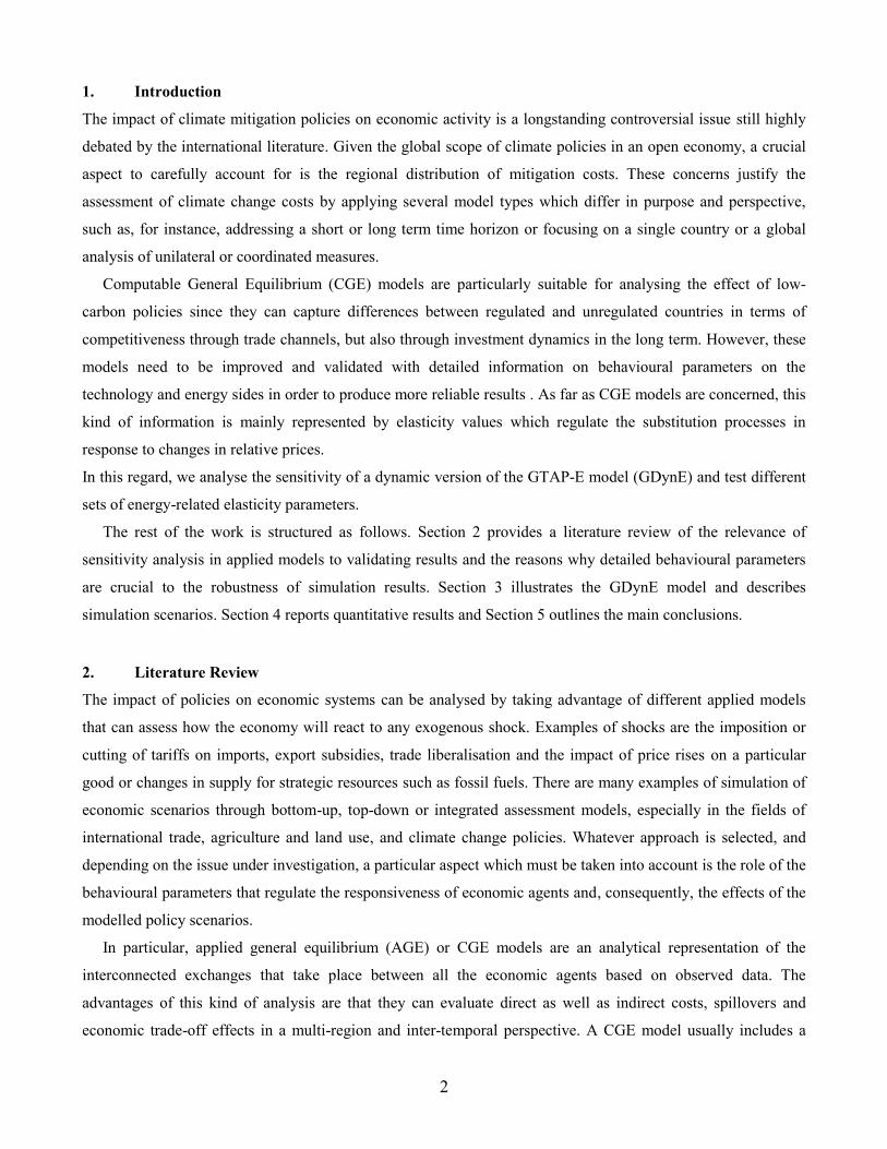
Figure 1 depicts the trends of CO2 emission pathways obtained in the two baselines (Case A and Case B),

together with the path of global emissions that should be achieved according to the 450 PPM scenario. In both

cases, we distinguish between Annex I and non-Annex I countries because, although the parameters assume the

same values in all regions, the overall impact is different across countries depending on the internal economic

structure. Emissions from baseline A are higher than in case B (there is a gap of 3 Gt CO2 in 2050), meaning that

the introduction of empirically-based behavioural parameters, which are lower than in the standard case, makes

the overall system less flexible and the substitution between energy and capital less easy. The gap between Case

A and B is mainly due to the difference in emissions from non-Annex I countries. This is partly due to the higher

growth rate these regions are characterised by, but is also a clear sign that the parameters sets are country

sensitive. In fact, it is also worth noting that, because the elasticities have the same values in all regions and

countries, the deviation between case A and B can also be explained by the different impacts that the parameters

have on each country given its internal economic structure. In particular, the distinction between Annex I and

non-Annex I countries highlights the crucial role played by energy-intensive activities and the fact that changes

in inter-fuel and energy-capital elasticities can produce differentiated impacts depending on the internal structure

of the country. For example, in the non-Annex I countries, China is responsible for a reduction in CO2 emissions

(in Case B compared with Case A) that is higher than for all the other non-Annex I countries put together.

Moreover, given that the exogenous shock to GDP is the same in both cases (A and B), the differences in

12

energy elasticities generate a different impact on overall regional efficiency and on the consumption of fossil

fuels. The endogenously determined factor augmenting technical change is higher in B than in A for all sectors

and is particularly high for the fossil fuel sectors.

Figure 1 - CO2 trends in 450PPM and BAU, Case A vs. Case B

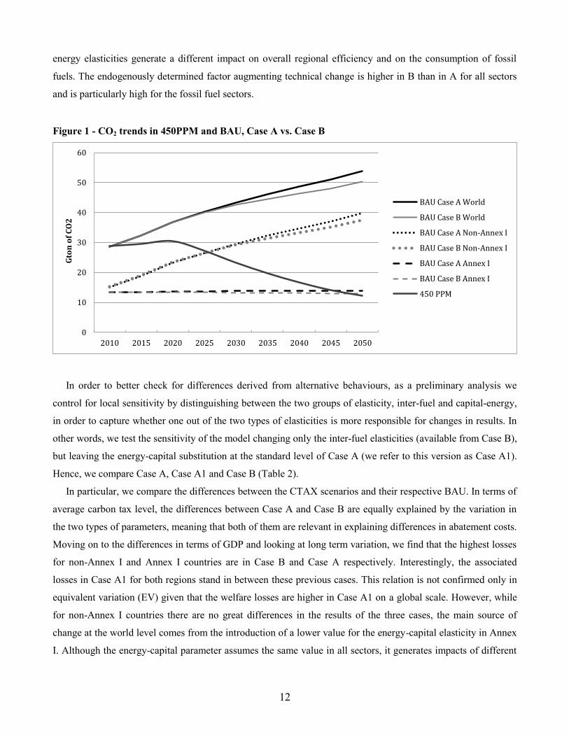
In order to better check for differences derived from alternative behaviours, as a preliminary analysis we

control for local sensitivity by distinguishing between the two groups of elasticity, inter-fuel and capital-energy,

in order to capture whether one out of the two types of elasticities is more responsible for changes in results. In

other words, we test the sensitivity of the model changing only the inter-fuel elasticities (available from Case B),

but leaving the energy-capital substitution at the standard level of Case A (we refer to this version as Case A1).

Hence, we compare Case A, Case A1 and Case B (Table 2).

In particular, we compare the differences between the CTAX scenarios and their respective BAU. In terms of

average carbon tax level, the differences between Case A and Case B are equally explained by the variation in

the two types of parameters, meaning that both of them are relevant in explaining differences in abatement costs.

Moving on to the differences in terms of GDP and looking at long term variation, we find that the highest losses

for non-Annex I and Annex I countries are in Case B and Case A respectively. Interestingly, the associated

losses in Case A1 for both regions stand in between these previous cases. This relation is not confirmed only in

equivalent variation (EV) given that the welfare losses are higher in Case A1 on a global scale. However, while

for non-Annex I countries there are no great differences in the results of the three cases, the main source of

change at the world level comes from the introduction of a lower value for the energy-capital elasticity in Annex

I. Although the energy-capital parameter assumes the same value in all sectors, it generates impacts of different

0

10

20

30

40

50

60

2010 2015 2020 2025 2030 2035 2040 2045 2050

Gto

n o

f C

O2

BAU Case A World

BAU Case B World

BAU Case A Non-Annex I

BAU Case B Non-Annex I

BAU Case A Annex I

BAU Case B Annex I

450 PPM

13

magnitude among regions, depending on the internal economic structure, and it seems to be highly relevant to

the regional distribution of policy impacts. This first result gives rise to the need for further research efforts to be

made in finding robust empirical estimations of behavioural parameters at the country level.

Table 2 – Comparison between Cases A, A1 and B applied to CTAX

2015 2020 2025 2030 2035 2040 2045 2050 Cumulated

Weighted average Carbon Tax level in CTAX (USD/ton of CO2)

Case A World 11 17 55 109 172 242 362 488

Non-Annex I 10 13 40 82 153 232 364 508

Annex I 13 23 82 163 211 263 356 438 Case A1 World 11 17 57 114 182 259 391 530

Non-Annex I 10 13 42 86 164 252 398 557

Annex I 12 23 85 169 219 275 375 465 Case B World 11 17 58 118 191 273 422 570

Non-Annex I 11 14 44 92 176 272 439 608

Annex I 11 21 84 171 222 277 383 477 Differences in GDP between CTAX and BAU (Bln USD)

Case A World -45 -162 -590 -1,563 -3,114 -5,344 -8,417 -12,311 -31,546

Non-Annex I -48 -175 -473 -1,055 -2,181 -3,970 -6,583 -10,195 -24,680

Annex I 3 13 -117 -508 -932 -1,374 -1,834 -2,116 -6,865

Case A1 World -45 -162 -603 -1,612 -3,245 -5,626 -8,956 -13,230 -33,479

Non-Annex I -46 -174 -478 -1,087 -2,298 -4,261 -7,179 -11,245 -26,768

Annex I 1 11 -125 -526 -947 -1,364 -1,777 -1,985 -6,712

Case B World -44 -156 -580 -1,553 -3,140 -5,438 -8,776 -13,172 -32,859

Non-Annex I -55 -216 -572 -1,256 -2,600 -4,737 -8,021 -12,673 -30,130

Annex I 12 60 -8 -296 -540 -700 -755 -499 -2,726

Differences in EV between CTAX and BAU (Bln USD) Case A World -117 -193 -1,410 -3,335 -6,000 -9,489 -11,415 -14,930 -46,889

Non-Annex I -83 -207 -1,075 -2,328 -4,441 -7,274 -8,772 -11,673 -35,854

Annex I -33 14 -335 -1,006 -1,559 -2,215 -2,643 -3,257 -11,035

Case A1 World -108 -177 -1,414 -3,414 -6,198 -9,919 -12,092 -15,902 -49,225

Non-Annex I -77 -199 -1,073 -2,377 -4,594 -7,684 -9,478 -12,741 -38,223

Annex I -32 22 -341 -1,037 -1,604 -2,235 -2,614 -3,162 -11,002

Case B World -99 -102 -1,249 -2,954 -5,281 -8,212 -9,739 -12,980 -40,616

Non-Annex I -78 -206 -1,060 -2,251 -4,311 -7,194 -8,962 -12,449 -36,513

Annex I -20 104 -189 -703 -970 -1,017 -777 -531 -4,103

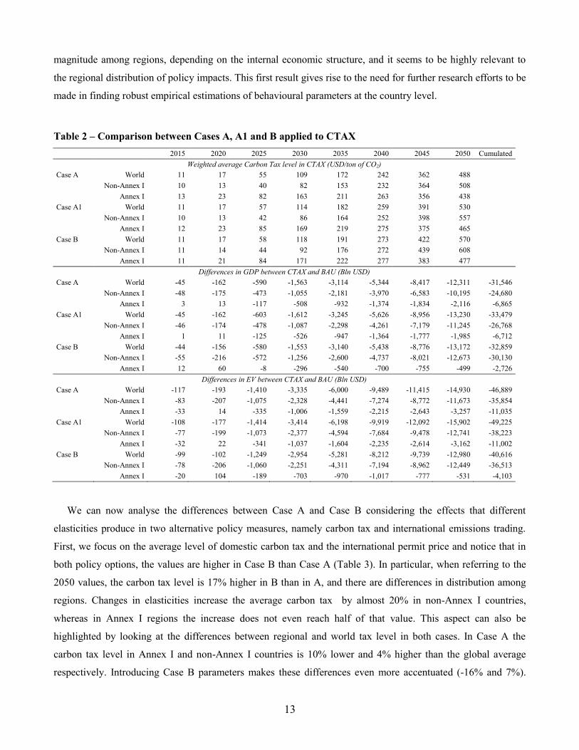
We can now analyse the differences between Case A and Case B considering the effects that different

elasticities produce in two alternative policy measures, namely carbon tax and international emissions trading.

First, we focus on the average level of domestic carbon tax and the international permit price and notice that in

both policy options, the values are higher in Case B than Case A (Table 3). In particular, when referring to the

2050 values, the carbon tax level is 17% higher in B than in A, and there are differences in distribution among

regions. Changes in elasticities increase the average carbon tax by almost 20% in non-Annex I countries,

whereas in Annex I regions the increase does not even reach half of that value. This aspect can also be

highlighted by looking at the differences between regional and world tax level in both cases. In Case A the

carbon tax level in Annex I and non-Annex I countries is 10% lower and 4% higher than the global average

respectively. Introducing Case B parameters makes these differences even more accentuated (-16% and 7%).

14

Finally, when comparing domestic carbon tax level and international permit prices, the percentage change at

world level remains stable between A and B (-16% and -17%). On the other hand, in Case B the carbon tax in

Annex I countries is only 1% higher than the permit price in the IET scenario (7% in Case A), whereas in non-

Annex I countries, the corresponding percentage change is 29% (24% in Case A).

Table 3 - Carbon tax level and permit price in 450PPM, Case A vs. Case B (USD/ton CO2)

2015 2020 2025 2030 2035 2040 2045 2050

Weighted average domestic carbon tax (CTAX)

Case A World 11 17 55 109 172 242 362 488

Non-Annex I 10 13 40 82 153 232 364 508

Annex I 13 23 82 163 211 263 356 438

Case B World 11 17 58 118 191 273 422 570

Non-Annex I 11 14 44 92 176 272 439 608

Annex I 11 21 84 171 222 277 383 477

International permit price (IET)

Case A World 7 11 46 104 170 225 320 410

Case B World 7 11 48 113 187 249 364 471

In addition to these relative changes, it is worth noting the link between the value of domestic carbon tax (or

permit price) and the actual amount of CO2 emission abated in each 450PPM scenario compared with the BAU

case. Considering that the level of emissions in the baseline is higher in Case A and the 450PPM targets are the

same irrespective of the elasticity values, although the amount of CO2 abated in Case B is lower, the costs per

ton of emission are higher than in Case A.

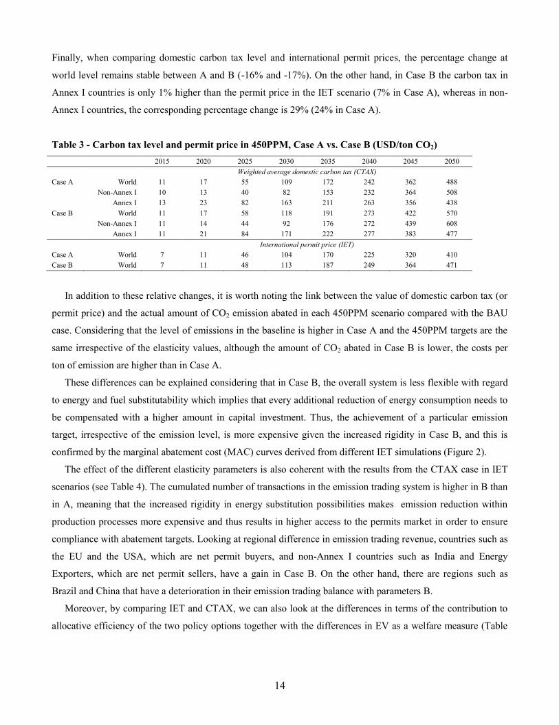
These differences can be explained considering that in Case B, the overall system is less flexible with regard

to energy and fuel substitutability which implies that every additional reduction of energy consumption needs to

be compensated with a higher amount in capital investment. Thus, the achievement of a particular emission

target, irrespective of the emission level, is more expensive given the increased rigidity in Case B, and this is

confirmed by the marginal abatement cost (MAC) curves derived from different IET simulations (Figure 2).

The effect of the different elasticity parameters is also coherent with the results from the CTAX case in IET

scenarios (see Table 4). The cumulated number of transactions in the emission trading system is higher in B than

in A, meaning that the increased rigidity in energy substitution possibilities makes emission reduction within

production processes more expensive and thus results in higher access to the permits market in order to ensure

compliance with abatement targets. Looking at regional difference in emission trading revenue, countries such as

the EU and the USA, which are net permit buyers, and non-Annex I countries such as India and Energy

Exporters, which are net permit sellers, have a gain in Case B. On the other hand, there are regions such as

Brazil and China that have a deterioration in their emission trading balance with parameters B.

Moreover, by comparing IET and CTAX, we can also look at the differences in terms of the contribution to

allocative efficiency of the two policy options together with the differences in EV as a welfare measure (Table

15

5). As expected, the contribution to allocative efficiency is higher in emission trading, in both Cases A and B,5

denoting that in a partial equilibrium perspective, IET is the most cost-effective solution among the available

mitigation policies. However, considering the general equilibrium effects at the cumulate level, as indicated by

the EV differences, only non-Annex I countries have net gains from emission trading policy, whereas at the

world level, the negative effect experienced by Annex I countries prevails resulting in a net loss and the gap

increases with Case B.

Figure 2 – Marginal Abatement Cost curves at the world level in IET scenario, Case A vs. Case B

Considering only non-Annex I countries, in 2025 and 2030, the contribution to allocative efficiency is higher

in the CTAX case, (the differences are negative) and this is due to the increasing stringency in the abatement

targets (especially for China and India). Nonetheless, the emission trading is still more cost effective at the

global level than the carbon tax measure. Considering the entire time period up to 2050, an emission trading

scenario seems to induce a strong restructuring of economic processes that starts immediately until the

abatement target becomes binding. On the other hand, in the CTAX case, losses in allocative efficiency due to

the reallocation of production factors are lower during the initial periods, but determine higher losses in the long

term.

5 This is also coherent with differences in GDP given that losses in emission trading are lower than in a domestic carbon tax case, in both cases A and B (see Table A.7 in Appendix).

2015 2020

2025

2030

2035

2040

2045

2050

0

100

200

300

400

500

600

0 5 10 15 20 25 30 35 40 45

US

D/

ton

CO

2

Gton of CO2 emissions abated per period (2010-2050)

450PPM Case A

450PPM Case B

16

Table 4 – Emission Trading Balance in IET scenario, Case A vs. Case B (Mln USD)

2015 2020 2025 2030 2035 2040 2045 2050 Cumulated

Emissions trading balance Case A

EU -470 -2,164 -17,266 -53,835 -90,993 -105,654 -120,742 -119,290 -510,414

USA -54 -451 -12,169 -47,581 -70,219 -65,489 -66,672 -64,161 -326,797

FSU -16 207 1,924 11,046 32,675 63,421 106,997 140,941 357,195

Other Annex I -755 -2,978 -16,911 -42,242 -65,941 -73,047 -78,907 -71,848 -352,630

Brazil -67 -231 -1,864 -4,698 -3,516 2,068 10,955 24,078 26,726

China 2,275 9,256 58,283 134,053 143,988 57,152 -68,341 -219,115 117,552

India 1,062 4,544 29,184 73,806 123,184 159,025 203,418 222,416 816,641

Energy Exporters -1,072 -4,399 -19,878 -23,054 2,172 53,859 134,739 227,301 369,668

Other non-Annex I -902 -3,785 -21,304 -47,494 -71,350 -91,335 -121,447 -140,322 -497,938

No. of transactions 3,337 14,008 89,392 218,906 302,019 335,525 456,109 614,737 2,034,031

Emissions trading balance Case B

EU -296 -1,309 -12,753 -45,717 -81,700 -95,825 -111,801 -109,978 -459,379

USA 148 601 -6,940 -39,547 -59,663 -51,313 -48,932 -43,039 -248,686

FSU -8 165 1,367 11,700 38,457 75,583 132,008 175,362 434,634

Other Annex I -737 -2,898 -17,346 -43,685 -67,665 -72,251 -76,641 -66,934 -348,157

Brazil -99 -357 -2,808 -6,944 -6,260 -73 9,701 24,253 17,412

China 2,033 8,125 54,330 127,270 126,709 17,474 -148,689 -347,717 -160,464

India 1,150 4,765 31,518 80,355 134,282 171,765 225,707 249,046 898,589

Energy Exporters -1,163 -4,823 -22,424 -27,276 -659 57,854 155,537 272,064 429,111

Other non-Annex I -1,028 -4,270 -24,943 -56,157 -83,502 -103,215 -136,891 -153,058 -563,065

No. of transactions 3,331 13,656 87,215 219,326 299,449 322,677 522,954 720,725 2,189,333

Focusing on emission trading scenarios, in Table 6 we highlight the results and analyse the differences

generated by the elasticity changes in Case B compared with Case A in terms of GDP, looking at the deviation

between the policy and baseline results. At the world level, GDP losses in IET scenarios compared with the

BAU level are quite similar in both Cases A and B. However, there are specular differences across regions, and

the introduction of Case B parameters generates higher losses in non-Annex I countries that are compensated by

gains in Annex I regions. In fact, while in non-Annex I countries the GDP losses are higher in B and increasingly

over time, for Annex I countries results go in the opposite direction. They have GDP gains up to 2030 with Case

A, but with Case B the benefits are higher and last up to 2035; from 2040, in both Cases A and B, Annex I

countries have GDP losses, even though they are lower in B. Despite the fact that in Case A there is a greater

amount of CO2 emissions to be reduced, the lower overall flexibility in the system associated with parameters B

makes the economic impact of the abatement policies greater and also affects the distribution of costs across

regions, in this case penalising non-Annex I countries.

However, leaving aside the differences between these two macro regions, the impact of different elasticity

values is heterogeneous when also considering single countries. As far as non-Annex I countries are concerned,

half of the overall loss is due to the GDP reduction which originated in China and in Case B this effect is even

more evident, with an increase in losses in Chinese GDP of 21% in B compared with A, whereas for all other

non-Annex I countries the corresponding variation is only 6% (Figure 3).

17

Table 5 – Comparison in allocative efficiency and EV, Case A vs. Case B (Bln USD)

2015 2020 2025 2030 2035 2040 2045 2050 Cumulated

Differences in allocative efficiency between IET and CTAX

Case A World 8 20 98 221 171 218 356 532 1,617

Non-Annex I 4 2 7 30 50 147 317 508 1,064

Annex I 4 18 91 192 122 70 40 16 553

Case B World 8 16 83 200 185 264 458 711 1,925

Non-Annex I 4 2 2 19 81 218 448 703 1,476

Annex I 3 13 81 182 105 46 10 8 449

Differences in EV IET and CTAX

Case A World 33 -15 227 56 -487 -942 -898 -218 -2,246

Non-Annex I 13 -78 -60 -384 -573 -370 510 1,732 790

Annex I 19 63 287 440 86 -573 -1,408 -1,951 -3,036

Case B World 23 -53 209 52 -496 -970 -907 -32 -2,173

Non-Annex I 14 -67 -20 -347 -555 -263 842 2,476 2,080

Annex I 9 14 229 399 60 -707 -1,749 -2,508 -4,253

Table 6 - Differences in GDP between Case A and Case B in IET scenario (Mln USD)

2015 2020 2025 2030 2035 2040 2045 2050 Cumulated

Differences in GDP (IET w.r.t. BAU) Case A

World -27 -91 -395 -1,212 -2,697 -4,822 -7,609 -10,896 -27,749

Non-Annex I -42 -166 -541 -1,328 -2,568 -4,215 -6,361 -9,078 -24,299

Annex I 15 75 146 117 -129 -607 -1,249 -1,818 -3,450

Differences in GDP (IET w.r.t. BAU) Case B

World -29 -91 -392 -1,208 -2,706 -4,828 -7,714 -11,196 -28,164

Non-Annex I -43 -177 -583 -1,455 -2,854 -4,702 -7,210 -10,466 -27,490

Annex I 15 86 191 247 148 -126 -504 -730 -674

Moreover, also within the Annex I regions, differences in GDP losses are quite heterogeneous. The only

region that benefits from IET mitigation policy is the EU, which also has an increase in GDP gains in Case B

compared to A (Figure 4). On the other hand, both FSU and USA are subject to GDP losses with regard to

baseline level but, whereas for the former the introduction of Case B elasticities worsens this loss, USA takes

advantage in terms of a lower reduction of GDP with regard to the baseline.

Given that one of the main advantages of Case B is the introduction of econometric based inter-fuel

elasticities of substitution, we are now going to analyse the difference in energy mix in terms of world total

consumption of energy commodities and highlight the differences between Case A and Case B in emission

trading policy.

Considering the structure of the production function, the upper nest describes the substitution between

electricity and non-electricity energy sources and the value of the corresponding elasticity parameter (ELFENY)

goes from 1 (Case A) to 0.81 (Case B). At the lower aggregation level, coal can be substituted with three other

non-electricity fuels (oil, oil products and natural gas) through the non-electricity elasticity of substitution

parameters (ELFENELY) which slightly increased from A to B (0.50 and 0.57, respectively). Finally, the non-

coal elasticity of substitution (ELFNCOAL), which determine the substitution between oil, oil products and

natural gas, drops from the value of 1 in Case A to 0.41 in Case B.

18

Figure 3 – Differences in Non-Annex I GDP between IET and BAU, Case A vs. Case B (Bln USD)

Figure 4 - Differences in Annex I GDP between IET and BAU, Case A vs. Case B (Bln USD)

When introducing less flexible elasticity parameters (Case B), we impose even more stringent boundaries on

the model. Therefore, there are differences in the percentage change between 2010 and 2050 in the baselines

where the increase (decrease) in energy consumption with Case B is lower (higher) than in Case A (see Table 7).

These variations determine changes in regional and sectoral energy demands also in the IET scenario. In

particular, the increase in electricity consumption is lower with Case B than with standard parameters (Case A)

at the world level, and the effect is particularly evident for non-Annex I countries.

World

Annex I

Non-Annex I

China Other non-Annex I

-30000

-25000

-20000

-15000

-10000

-5000

0

Case A Case B

Canada

EU

FSU

Norway

USA

Rest of Annex I

-4000

-3000

-2000

-1000

0

1000

2000

3000

4000

5000

6000

Case A Case B

19

Table 7 – Changes in fuel mix between 2010 and 2050 (Case A vs. Case B)

Coal Oil Natural gas Oil

products Electricity Total

BAU Case A World 58% -16% 57% 115% 181% 75%

Annex I -42% -47% 0% 31% 39% -1%

Non-Annex I 107% 21% 137% 217% 361% 153%

IET Case A World -79% -66% -70% -21% 93% -36%

Annex I -90% -76% -80% -47% -20% -62%

Non-Annex I -74% -53% -55% 11% 237% -9%

BAU Case B World 39% -19% 50% 107% 155% 63%

Annex I -52% -50% -6% 24% 28% -8%

Non-Annex I 84% 18% 130% 207% 315% 136%

IET Case B World -79% -67% -68% -24% 71% -40%

Annex I -90% -78% -79% -52% -26% -65%

Non-Annex I -73% -54% -53% 11% 193% -14%

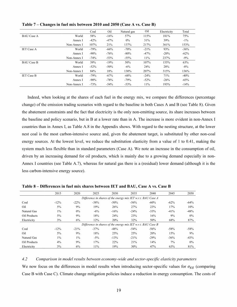
Indeed, when looking at the shares of each fuel in the energy mix, we compare the differences (percentage

change) of the emission trading scenarios with regard to the baseline in both Cases A and B (see Table 8). Given

the abatement constraints and the fact that electricity is the only non-emitting source, its share increases between

the baseline and policy scenario, but in B at a lower rate than in A. The increase is more evident in non-Annex I

countries than in Annex I, as Table A.8 in the Appendix shows. With regard to the nesting structure, at the lower

nest coal is the most carbon-intensive source and, given the abatement target, is substituted by other non-coal

energy sources. At the lowest level, we reduce the substitution elasticity from a value of 1 to 0.41, making the

system much less flexible than in standard parameters (Case A). We note an increase in the consumption of oil,

driven by an increasing demand for oil products, which is mainly due to a growing demand especially in non-

Annex I countries (see Table A.7), whereas for natural gas there is a (residual) lower demand (although it is the

less carbon-intensive energy source).

Table 8 – Differences in fuel mix shares between IET and BAU, Case A vs. Case B

2015 2020 2025 2030 2035 2040 2045 2050

Difference in shares of the energy mix IET w.r.t. BAU Case A

Coal -12% -22% -38% -50% -56% -60% -62% -64%

Oil 5% 9% 19% 26% 27% 23% 17% 10%

Natural Gas 1% 0% -6% -16% -24% -33% -41% -48%

Oil Products 5% 9% 18% 24% 23% 16% 9% 0%

Electricity 3% 6% 12% 20% 32% 50% 68% 87%

Difference in shares of the energy mix IET w.r.t. BAU Case B

Coal -12% -21% -37% -48% -54% -56% -58% -58%

Oil 5% 9% 18% 25% 25% 20% 15% 9%

Natural Gas 1% 1% -5% -13% -21% -29% -36% -43%

Oil Products 4% 9% 17% 22% 21% 14% 7% 0%

Electricity 3% 6% 11% 19% 30% 47% 63% 81%

4.2 Comparison in model results between economy-wide and sector-specific elasticity parameters

We now focus on the differences in model results when introducing sector-specific values for (comparing

Case B with Case C). Climate change mitigation policies induce a reduction in energy consumption. The costs of

20

achieving a reduction in energy intensity are strongly influenced by the flexibility of each sector in substituting

energy with other inputs. Therefore, by using specific values, the distribution of mitigation costs may vary

substantially across different sectors.

First, we report in Table A.9 in the Appendix the carbon intensity of manufacturing sectors which are those

where values have changed from B to C. In particular, we specify the 2010 carbon intensity (which is

common to every scenarios) together with the 2050 level, and distinguish between Case B and Case C, as well as

between IET and BAU scenarios.

Results from BAU show that the most carbon-intensive sectors are the Non-metallic minerals, Basic metals,

Chemicals and Paper industries, but also have the most significant differences between the two regions

considered in this analysis (Annex I and non-Annex I). Given that the abatement targets are the same in both

Cases B and C, results from policy scenarios are more homogeneous and we can focus on the specific

differences induced by the different elasticity sets by looking at the percentage changes between the results from

IET and BAU scenarios in 2050. In this case, at the world level the reduction in carbon intensity with Case C

values is higher (lower) for all sectors where has increased (decreased) compared with Case B. The greatest

reductions in carbon intensity are in the Food and Textile sectors, with a quite homogeneous difference across

regions. On the other hand, there are significant positive changes in the Wood and Other manufacturing sectors,

mainly for Annex I countries, and in the Basic metals sector, especially in non-Annex I regions.

It is worth mentioning that in the Paper sector, whose has the same value in B and C, we note a negative

difference for non-Annex I countries and at the world level, while in the Annex I region, the difference is almost

zero. Moreover, it is interesting to look at changes in Chemicals sector: there is a negative change in Annex I

region (-0.17) and a positive one for non-Annex I countries (1.16), resulting in a positive variation at the world

aggregate level. In this case, it is clear how differences in flexibility in energy use may generate different

impacts depending on the internal economic structure. In fact, if we look at the whole manufacturing sector, in

Annex I countries we found a negative change (-0.45) whereas the same relation in non-Annex I countries

highlights a positive difference (0.43). This leads to the fact that, although the changes in parameters are the

same for all countries, there are regional differences and the reduction in carbon intensity has been relatively

greater for Annex I economies with Case C, while the opposite holds for non-Annex I countries. Thus, at the

aggregate level, in the sectors where the parameters in C are higher than in B (meaning greater technological

flexibility), the carbon intensity is always lower than in corresponding sectors with Case B. However, at a more

disaggregated regional level, an increase in substitutability is not necessarily linked to a reduction in carbon

intensity and a different distribution of abatement costs occurs.

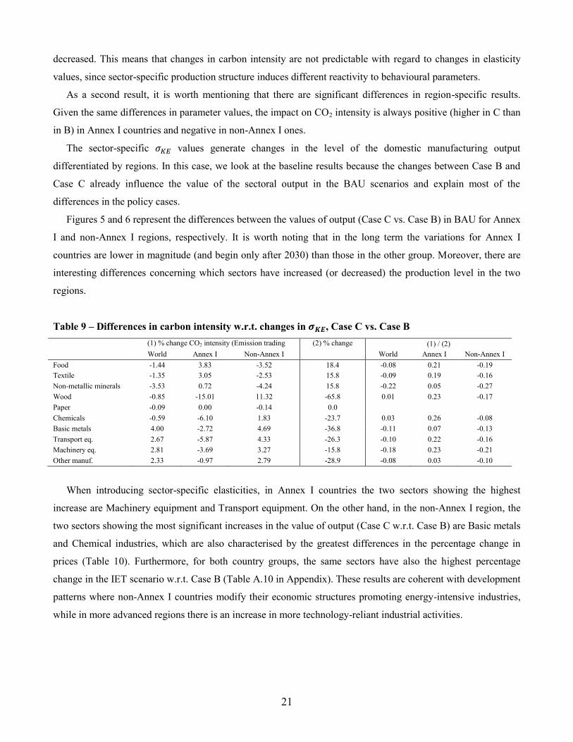
Table 9 shows the differences in output compared with the differences in the value as a ratio between the

percentage change in CO2 intensity between Case C and B (at 2050 for IET scenario) and the percentage change

in . As a first general remark, at the world level, in each sector where has increased in Case C w.r.t. Case

B, the relative CO2 intensity is lower, while the same conclusion does not hold for sectors where elasticity has

21

decreased. This means that changes in carbon intensity are not predictable with regard to changes in elasticity

values, since sector-specific production structure induces different reactivity to behavioural parameters.

As a second result, it is worth mentioning that there are significant differences in region-specific results.

Given the same differences in parameter values, the impact on CO2 intensity is always positive (higher in C than

in B) in Annex I countries and negative in non-Annex I ones.

The sector-specific values generate changes in the level of the domestic manufacturing output

differentiated by regions. In this case, we look at the baseline results because the changes between Case B and

Case C already influence the value of the sectoral output in the BAU scenarios and explain most of the

differences in the policy cases.

Figures 5 and 6 represent the differences between the values of output (Case C vs. Case B) in BAU for Annex

I and non-Annex I regions, respectively. It is worth noting that in the long term the variations for Annex I

countries are lower in magnitude (and begin only after 2030) than those in the other group. Moreover, there are

interesting differences concerning which sectors have increased (or decreased) the production level in the two

regions.

Table 9 – Differences in carbon intensity w.r.t. changes in , Case C vs. Case B

(1) % change CO2 intensity (Emission trading scenario, 2050)Case C vs Case B

(2) % change EK_sub

(1) / (2)

World Annex I Non-Annex I

World Annex I Non-Annex I

Food -1.44 3.83 -3.52 18.4 -0.08 0.21 -0.19

Textile -1.35 3.05 -2.53 15.8 -0.09 0.19 -0.16

Non-metallic minerals -3.53 0.72 -4.24 15.8 -0.22 0.05 -0.27

Wood -0.85 -15.01 11.32 -65.8 0.01 0.23 -0.17

Paper -0.09 0.00 -0.14 0.0

Chemicals -0.59 -6.10 1.83 -23.7 0.03 0.26 -0.08

Basic metals 4.00 -2.72 4.69 -36.8 -0.11 0.07 -0.13

Transport eq. 2.67 -5.87 4.33 -26.3 -0.10 0.22 -0.16

Machinery eq. 2.81 -3.69 3.27 -15.8 -0.18 0.23 -0.21

Other manuf. 2.33 -0.97 2.79 -28.9 -0.08 0.03 -0.10

When introducing sector-specific elasticities, in Annex I countries the two sectors showing the highest

increase are Machinery equipment and Transport equipment. On the other hand, in the non-Annex I region, the

two sectors showing the most significant increases in the value of output (Case C w.r.t. Case B) are Basic metals

and Chemical industries, which are also characterised by the greatest differences in the percentage change in

prices (Table 10). Furthermore, for both country groups, the same sectors have also the highest percentage

change in the IET scenario w.r.t. Case B (Table A.10 in Appendix). These results are coherent with development

patterns where non-Annex I countries modify their economic structures promoting energy-intensive industries,

while in more advanced regions there is an increase in more technology-reliant industrial activities.

22

Figure 5 – Differences in output in BAU for Annex I countries, Case C vs. Case B

Figure 6 – Differences in output in BAU for non-Annex I countries, Case C vs. Case B

Table 10 – Differences in price changes in BAU, Case C vs. Case B (2050)

Case B (% change)* Case C (% change)* Diff. Case C – Case B

Annex I Non-Annex I Annex I Non-Annex I Annex I Non-Annex I

Food 9.89 8.44 9.84 8.37 -0.05 -0.07

Textile 3.10 4.13 3.07 4.09 -0.02 -0.04

Non-metallic minerals -0.02 1.45 -0.08 1.39 -0.06 -0.06

Wood 7.37 7.96 7.41 7.94 0.04 -0.02

Paper 2.90 1.74 2.93 1.74 0.03 0.00

Basic metals -4.17 -0.53 -3.99 -0.42 0.19 0.11

Chemicals -2.94 -2.93 -2.74 -2.75 0.20 0.18

Transport eq. 0.90 -0.41 0.94 -0.34 0.04 0.07

Machinery eq. 0.89 -0.43 0.93 -0.38 0.04 0.05

Other manuf. 3.42 1.58 3.46 1.65 0.05 0.07

Note: * The % changes are expressed in relation to the 2045 level.

-80

-60

-40

-20

0

20

40

60

80

2015 2020 2025 2030 2035 2040 2045 2050Bln

US

D

Food

Textile

Non-metallic minerals

Wood

Paper

Chemicals

Transport eq.

Machinery eq.

Other manuf.

Basic metals

-80

-60

-40

-20

0

20

40

60

80

2015 2020 2025 2030 2035 2040 2045 2050Bln

US

D

Food

Textile

Non-metallic minerals

Wood

Paper

Chemicals

Transport eq.

Machinery eq.

Other manuf.

Basic metals

23

Furthermore, when considering a mitigation policy scenario such as IET, there is still high variability

between the two macro-regions especially in the selected sectors shown in Figure 7 (Basic metals and Chemical

industries, but also less energy-intensive ones). In non-Annex I countries, the two sectors whose values of output

have the most relevant increase (Case C vs. Case B), are still Basic metals and Chemicals. On the other hand, the

only two sectors where the Annex I region experiences an increase in the output value are Machinery and

Transport equipment. Chemicals, Basic metals and Machinery equipment are also sectors where the changes in

elasticity parameters (Case C vs. Case B) produce the greatest variation in terms of carbon intensity between

non-Annex I and Annex I countries with regard to the global result.

It is also worth mentioning that the results in terms of value of export (Figure 8) for energy-intensive sectors,

especially Chemicals and Basic metals, are reasonably in line with those on output, whereas there are greater

differences for the other sectors due to trade dynamics.

Figure 7 – Differences in output in IET (cumulated 2010-2050), Case C vs. Case B

Figure 8 – Differences in export flows in IET (cumulated 2010-2050),Case C vs. Case B

-100

-50

0

50

100

150

Basic metals Chemicals Food Machinery eq. Non metallicminerals

Transport eq.

Bln

US

D

Annex I Non-Annex I

-100

0

100

200

300

400

500

600

700

Basic metals Chemicals Food Machinery eq. Non metallicminerals

Transport eq.

Bln

US

D

Annex I Non-Annex I

24

5. Conclusion

The aim of this work was to analyse the sensitivity of the energy version of the GDynE, a dynamic CGE model

that specifically accounts for economic and energy data, where we introduced sector-specific and

econometrically estimated values for the elasticity of substitution between capital and energy and between fuels.

Although this type of model is notably appropriate for addressing the economic impacts of climate mitigation

policies, it also needs detailed, reliable information on technology, energy and emissions linkages in order to

improve and validate results. We focused on two classes of behavioural parameters: the elasticity of substitution

between energy and capital and between different types of energy sources (inter-fuel substitution).

We considered three different sets of elasticity parameters: Case A, including standard values available from

the GTAP Database; Case B, including elasticity parameters derived from empirically estimated values

elaborated by a meta-analysis approach; Case C, including the same values adopted for Case B where

parameters are sector-specific econometrically estimated values.

We made comparisons between baselines and two alternative mitigation policies, a domestic carbon tax and

an international emission trading system, and allowed the target of limiting the concentration of GHGs in the

atmosphere to around 450 PPM of CO2 equivalent by 2050 to be reached.

When analysing the sensitivity of the model, we accounted for the impacts of changes in substitution

elasticities on abatement costs, the distribution of the effects among countries and sectors and the cost

effectiveness of the different policy measures.

First, the two types of parameters are both responsible for the variation in results and the different distribution

of impacts. A reduction in the flexibility of energy substitution possibilities makes abatement efforts more

expensive. In fact, considering both policy measures, the level of carbon tax and permit price is higher for Case

B w.r.t. Case A and the upward shift of the MAC curves confirms that, irrespective of the emissions level, the

increased rigidity makes the achievement of abatement targets more expensive. The limited possibilities to

increase energy consumption, especially for non-Annex I countries, and the consequent changes in fuel mix,

justify the greater losses in terms of GDP.

Second, restrictions in substitution possibilities in the energy nests generate changes in the distribution of

costs associated with the abatement efforts with regard to the two aggregate regional groups. This finding is

confirmed by all the economic impacts analysed such as differences in GDP, allocative efficiency, and welfare

levels. With regard to GDP, a restriction in flexibility generates opposite differences across the two regional

groups and the higher losses in non-Annex I countries are compensated for by gains in the Annex I regions.

Within each group there are also different responses to the same changes in elasticities, as in the case of China

and the European Union.

Third, when accounting for the elasticity of substitution between energy and capital differentiated by sector,

the model is again sensitive to the introduced changes both considering the climate and economic dimensions.

Changes in elasticities have large impacts in terms of distributive effects, given that there are significant

25

differences in carbon intensity and the value of production across sectors and regions. Even if the sector-specific

elasticities assume the same values in all countries, the effects between Annex I and non-Annex I regions are

rather different. In fact, changes in flexibility in energy use generate different regional impacts and the internal

economic structure can intensify the differences induced by the sectoral parameters.

Two main implications follow from this analysis. First, when considering the allocation of abatement targets

between different sectors within a country, heterogeneity in the technological flexibilities should also be taken

into consideration. Second, it is worth noting that further improvements to this type of model are highly

recommended in order to increase the reliability of simulation results. In particular, given the regional

differences in reacting to common sector-specific elasticity values, there is a need to empirically estimate all

energy-related behavioural parameters at the specific sector and country level with the highest disaggregation

compatible with data availability.

Acknowledgements

Financial support from the European Union D.G. Research with Grant Agreement number 283002 to the

research project ―Environmental Macro Indicators of Innovation‖ (EMInInn), the Roma Tre University-INEA-

ENEA Consortium, and from the Italian Ministry of Education, University and Research (Scientific Research

Program of National Relevance 2010 on ―Climate change in the Mediterranean area: scenarios, economic

impacts, mitigation policies and technological innovation‖) is gratefully acknowledged. The usual disclaimer

applies.

References

Alexeeva-Talebi, V., Böhringer, C., Löschel, A., Voigt, S., 2012. The value-added of sectoral disaggregation: Implication

on competitive consequences of climate change policies. Energy Economics, 34, 127-142.

Antimiani, A., Costantini, V., Martini, C., Palma, A., Tommasino, M.C., 2013a. The GTAP-E: model description and

improvements, in Costantini V., Mazzanti, M., (Eds.), 2013, The Dynamics of Environmental and Economic Systems.

Innovation, Environmental Policy and Competitiveness, Springer-Verlag, Berlin, 3-24.

Antimiani, A., Costantini, V., Martini, C., Salvatici, L., Tommasino, C., 2013b. Assessing alternative solutions to carbon

leakage. Energy Economics, 36, 299–311.

Antimiani, A., Costantini, V., Markandya, A., Martini, C., Palma, A., Tommasino, M.C., 2014. Green Growth and

sustainability: Analysing Trade-offs in Climate Change Policy Options. Seeds Working Paper 17/2014.

Beckman, J., Hertel, T., Tyner, W., 2011. Validating energy-oriented CGE models. Energy Economics, 33, 799-806.

Borghesi, S., 2011. The European emission trading scheme and renewable energy policies: credible targets for incredible

results?,International Journal of Sustainable Economy, 3, 312–327.

Broadstock D.C., Hunt L., Sorrel S., 2007. Elasticity of Substitution Studies, Review of Evidence for the Rebound Effect.

Technical Report 3, UK Energy Research Centre, London.

Burniaux, J-M., Martins, J.O., 2012. Carbon Leakages: a general equilibrium view. Economic Theory 49 (2), 473-495.

Burniaux, J.-M.,Truong T., 2002. GTAP-E: An Energy-Environmental Version of the GTAP Model. GTAP Technical

Paper No. 16. Center for Global Trade Analysis, Department of Agricultural Economics, Purdue University.

Capellán-Pérez, I., González-Eguino, M., Arto, I., Ansuategi, A., Dhavala, K., Patel, P., Markandya, A., (2014), New

climate scenario framework implementation in the GCAM integrated assessment model, BC3 Working Paper Series No.

2014-04.

26

Cariboni, J., Gatelli, D., Liska, R., Saltelli, A., 2007. The role of sensitivity in ecological modelling. Ecological Modelling,

203, 167-182.

Caron, J., 2012. Estimating carbon leakage and the efficiency of border adjustments in general equilibrium—Does sectoral

aggregation matter?.Energy Economics, 34, S111-S126.

Costantini, V., Paglialunga, E., 2014. Elasticity of substitution in capital-energy relationships: how central is a sector-based

panel estimation approach?. Seeds Working Paper 13/2014.

de Beer, J. (2000), Potential for Industrial Energy-Efficiency Improvement in the Long Term, Kluwer Academic Publisher,

Dordrecht, The Netherlands.

Golub, A., 2013. Analysis of Climate Policies withGDyn-E, GTAP Technical Papers No. 32.Center for Global Trade

Analysis, Department of Agricultural Economics, Purdue University.

Grubb, M., Edmonds, J., ten Brink, P., Morrison, M., 1993. The Cost of Limiting Fossil Fuel CO2 Emissions: A Survey and

an Analysis. Annual Review of Energy and the Environment, 18, 397-478.

Hamby, D.M., 1994. A review of techniques for parameter sensitivity analysis of environmental models. Environmental

Monitoring and Assessment, 32, 135-154.

Hertel, T.W., 1997. Global Trade Analysis:modeling and applications. Cambridge University Press.

Hertel, H., Hummels, D., Ivanic, M., Keeney, R., 2003. How confident can we be in CGE-Based Assessments of Free Trade

Agreements?, GTAP Working Papers 26, Center for Global Trade Analysis, Department of Agricultural Economics,

Purdue University.

Hillberry, H., Hummels, D., 2013. Trade Elasticity Parameters for a Computable General Equilibrium Model. Handbook of

Computable General Equilibrium Modeling, 1, 1213–1269.

Ianchovichina, E., McDougall R., 2000. Theoretical Structure of Dynamic GTAP. GTAP Technical Paper No. 17, Center

for Global Trade Analysis, Department of Agricultural Economics, Purdue University.

International Energy Agency (IEA), 2013. World Energy Outlook (WEO) 2013, International Energy Agency, Paris.

Intergovernmental Panel on Climate Change (IPCC), 2013. Fifth Assessment Report: Climate Change 2013, IPCC

Secretariat, Geneva, Switzerland.

Jacoby, H.D., Reilly, J.M., McFarland, J.R., Paltsev, S., 2004. Technology and Technical Change in the MIT EPPA Model.

MIT Joint Program on the Science and Policy of Global Change, Report No. 11, Cambridge, Massachusetts

Kemfert C., 1998. Estimated Substitution Elasticities of a Nested CES Production Function Approach for Germany. Energy

Economics, 20, 249- 264.

Koetse, M.J., de Groot, H.L.F., Florax, R.J.G.M., 2008. Capital-energy substitution and shifts in factor demand: A meta-

analysis. Energy Economics, 30, 2236-2251.

Kuik, O., Hofkes, M., 2010. Border adjustment for European emission trading: Competitiveness and carbon leakage. Energy

Policy, 38, 1741-1748.

Lecca, P., Swales, K., Turner, K., 2011. An investigation of issues relating to where energy should enter the production

function. Economic Modelling, 28, 2832-2841.

Löschel, A., 2002. Technological change in economic models of environmental policy: a survey. Ecological Economics, 43

(2-3), 105-126.

Mary, S., Phimister, E., Roberts, D., Santini, F., 2013. Testing the sensitivity of GCE results: A Monte Carlo Filtering

approach to an application to rural development policies in Aberdeenshire. JRC-IPTS Working Paper No. JRC85290,

JRC Scientific and Policy Reports.

McDougall R., Golub A., 2007. GTAP-E: A Revised Energy-Environmental Version of the GTAP Model. GTAP Research

Memorandum No. 15, Center for Global Trade Analysis, Department of Agricultural Economics, Purdue University.

Németh, G., Szabó, L., Ciscar, J-C., 2011. Estimation of Armingtonelasticities in a CGE economy–energy–environment

model for Europe. Economic Modelling, 28, 1993-1999.

Nijkamp, P., Wang, S., Kremers, H., 2005. Modeling the impacts of international climate change policies in a CGE context:

the use of the GTAP-E model. Economic Modelling, 22, 955–974.

Okagawa, A., Ban, K., 2008. Estimation of substitution elasticities for CGE models. Discussion Papers in Economics and

Business 08-16, Osaka University, Graduate School of Economics and Osaka School of International Public Policy

(OSIPP).

Quillet, A., Frolking, S., Garneau, M., Talbot, J., Peng, C., 2013. Assessing the role of parameter interactions in sensitivity

27

analysis of a model of peatland dynamics. Ecological Modelling, 248, 30-40.

Saltelli, A., Ratto, M., Andres, T., Campolongo, F., Carboni, J., Gatelli, D., Saisana, M., Tarantola, S., 2008. Global

Sensitivity Analysis: the primer. John Wiley & Sons, 2008.

Siddig, K., Grethe, H., 2014. International price transmission in CGE models: How to reconcile econometric evidence and

endogenous model response? Economic Modelling, 38, 12-22.

Springer, K., 2002. Climate Policy in a Globalizing world: A CGE Model with Capital Mobility and Trade(Vol. 320).

Springer Science & Business Media.

Stern D., 2012. Interfuel substitution: A meta-analysis. Journal of Economic Surveys, 26, 2, 307–331.

vanVuuren, D. P., Edmonds, J., Kainuma, M., Riahi, K., Thomson, A., Hibbard, K., Hurtt, G. C., Kram, T., Krey, V.,

Lamarque, J. -F., Masui, T., Meinshausen, M., Nakicenovic, N., Smith, S. J., and Rose, S. K., 2011. The representative

concentration pathways: an overview. Climatic Change,109, 5-31.

28

Appendix

Table A.1 - List of GDYnE countries

GTAP

code

Cod

e Country

GTA

P

code

Cod

e Country

GTAP

code Code Country

BRA bra Brazil EU27 mlt Malta RAM gtm Guatemala

CAN can Canada EU27 nld Netherlands RAM hnd Honduras

CHN chn China EU27 pol Poland RAM nic Nicaragua

CHN hkg Hong Kong EU27 prt Portugal RAM pan Panama

EExAf xcf Central Africa EU27 rou Romania RAM pry Paraguay

EExAf egy Egypt EU27 svk Slovakia RAM per Peru

EExAf nga Nigeria EU27 svn Slovenia RAM xca Rest of Central America

EExAf xnf Rest of North Africa EU27 esp Spain RAM xna Rest of North America

EExAf zaf South Africa EU27 swe Sweden RAM xsm Rest of South America

EExAf xac South Central Africa EU27 gbr United Kingdom RAM ury Uruguay

EExA

m arg Argentina FSU blr Belarus RAS arm Armenia

EExA

m bol Bolivia FSU rus Russian Federation RAS bgd Bangladesh

EExAm

col Colombia IDN idn Indonesia RAS bhr Bharain

EExA

m ecu Ecuador IND ind India RAS khm Cambodia

EExAm

ven Venezuela JPN jpn Japan RAS kgz Kyrgyztan

EExAs aze Azerbaijan KOR kor Korea RAS lao Lao People's Democratic Rep.

EExAs irn Iran Islamic Republic

of MEX mex Mexico RAS mng Mongolia

EExAs kaz Kazakhstan NOR nor Norway RAS npl Nepal

EExAs kwt Kuwait RAF bwa Botswana RAS xea Rest of East Asia

EExAs mys Malaysia RAF cmr Cameroon RAS xoc Rest of Oceania

EExAs omn Oman RAF civ Cote d'Ivoire RAS xsa Rest of South Asia

EExAs qat Qatar RAF eth Ethiopia RAS xse Rest of Southeast Asia

EExAs xsu Rest of Former Soviet

Union RAF gha Ghana RAS sgp Singapore

EExAs xws Rest of Western Asia RAF ken Kenya RAS lka Sri Lanka

EExAs sau Saudi Arabia RAF mdg Madagascar RAS twn Taiwan

EExAs are United Arab Emirates RAF mwi Malawi RAS pak Pakistan

EU27 aut Austria RAF mus Mauritius RAS phl Philippines

EU27 bel Belgium RAF moz Mozambique RAS tha Thailand

EU27 bgr Bulgaria RAF nam Namibia RAS vnm Vietnam

EU27 cyp Cyprus RAF xec Rest of Eastern Africa REU alb Albania

EU27 cze Czech Republic RAF xsc Rest of South African Custom

REU hrv Croatia

EU27 dnk Denmark RAF xwf Rest of Western Africa REU geo Georgia

EU27 est Estonia RAF sen Senegal REU xee Rest of Eastern Europe

EU27 fin Finland RAF tza Tanzania REU xef Rest of EFTA

EU27 fra France RAF uga Uganda REU xer Rest of Europe

EU27 deu Germany RAF zmb Zambia REU xtw Rest of the World

EU27 grc Greece RAF zwe Zimbabwe REU tur Turkey

EU27 hun Hungary RAF mar Morocco REU ukr Ukraine

EU27 irl Ireland RAF tun Tunisia ROEC

D aus Australia

EU27 ita Italy RAM xcb Caribbean ROECD

isr Israel

EU27 lva Latvia RAM chl Chile ROEC

D nzl New Zealand

EU27 ltu Lithuania RAM cri Costa Rica ROEC

D che Switzerland

EU27 lux Luxembourg RAM slv El Salvador USA usa United States of America

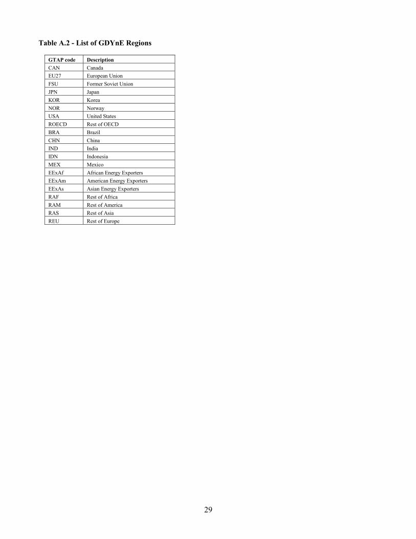
29

Table A.2 - List of GDYnE Regions

GTAP code Description

CAN Canada

EU27 European Union

FSU Former Soviet Union

JPN Japan

KOR Korea

NOR Norway

USA United States

ROECD Rest of OECD

BRA Brazil

CHN China

IND India

IDN Indonesia

MEX Mexico

EExAf African Energy Exporters

EExAm American Energy Exporters

EExAs Asian Energy Exporters

RAF Rest of Africa

RAM Rest of America

RAS Rest of Asia

REU Rest of Europe

30

Table A.3 - List of GDYnE commodities and aggregates

Sector Code Products Sector Code Products

agri pdr paddy rice wood lum wood products

agri wht wheat paper ppp paper products, publishing

agri gro cereal grains nec oil_pcts p_c petroleum, coal products

agri v_f vegetables, fruit, nuts chem crp chemical, rubber, plastic

products

agri osd oil seeds nometal nmm mineral products nec

agri c_b sugar cane, sugar beet basicmet i_s ferrous metals

agri pfb plant-based fibers basicmet nfm metals nec

agri ocr crops nec basicmet fmp metal products

agri ctl bovine cattle, sheep and goats,

horses transeqp mvh motor vehicles and parts

agri oap animal products nec transeqp otn transport equipment nec

agri rmk raw milk macheqp ele electronic equipment

agri wol wool, silk-worm cocoons macheqp ome machinery and equipment nec

agri frs forestry oth_man_ind omf manufactures nec

agri fsh fishing electricity ely electricity

Coal coa coal gas gdt gas manufacture, distribution

Oil oil oil services wtr water

Gas gas gas services cns construction

nometal omn minerals nec services trd trade

food cmt bovine cattle, sheep and goat

meat products transport otp transport nec

food omt meat products wat_transp wtp water transport

food vol vegetable oils and fats air_transp atp air transport

food mil dairy products services cmn communication

food pcr processed rice services ofi financial Oth_Ind_sericesnec

food sgr sugar services isr insurance

oth_man_ind ofd Oth_Ind_ser products nec services obs business and other services nec

food b_t beverages and tobacco products services ros recreational and other services

textile tex textiles services osg public admin. and defence,

education, health

textile wap wearing apparel services dwe ownership of dwellings

textile lea leather products

31

Table A.4 - List of GDYnE aggregates

Sector Full description

agri Agriculture

food Food

coal Coal

oil Oil

gas Gas

oil_pcts Petroleum, coal products

electricity Electricity

text Textile

nometal Non-metallic mineral products

wood Wood

paper Pulp and paper

chem Chemical and petrochemical

basicmet Basic metal

transeqp Transport equipment

macheqp Machinery and equipment

oth_man_ind Other manufacturing industries

transport Transport

wat_transp Water Transport

air_transp Air Transport

services Services

32

Table A.5 - Baseline GDP Projections to 2050 (Billion constant USD)

2010 2015 2020 2025 2030 2035 2040 2045 2050

Growth

p.a.

Canada 1,424 1,668 1,893 2,092 2,286 2,493 2,707 2,924 3,145 2.1%

European Union 16,489 18,302 20,051 21,451 22,627 23,714 24,823 25,943 27,080 1.3%

Former Soviet Union 1,344 1,589 1,858 2,105 2,346 2,580 2,782 2,937 3,065 2.2%

Japan 4,186 4,575 4,895 5,173 5,379 5,500 5,546 5,592 5,641 0.8%

Korea 1,100 1,316 1,474 1,595 1,686 1,759 1,817 1,863 1,896 1.4%

Norway 393 427 472 522 572 621 672 728 786 1.8%

United States 13,947 15,868 17,779 19,633 21,548 23,565 25,656 27,799 29,986 2.0%

Rest of OECD 1,646 1,861 2,071 2,267 2,459 2,660 2,872 3,099 3,330 1.8%

Brazil 1,474 1,753 2,077 2,421 2,775 3,137 3,500 3,863 4,223 2.8%

China 4,687 7,157 10,602 15,128 20,630 26,893 33,517 40,130 46,321 6.8%

India 1,482 2,091 2,925 4,068 5,591 7,558 9,996 12,872 16,119 7.0%

Indonesia 498 648 848 1,104 1,421 1,802 2,250 2,769 3,361 5.4%

Mexico 995 1,233 1,478 1,733 1,985 2,219 2,432 2,636 2,830 2.8%

African Energy Exp. 889 1,117 1,408 1,785 2,273 2,902 3,702 4,722 6,039 5.4%

American Energy Exp. 801 942 1,126 1,326 1,542 1,772 2,014 2,266 2,525 3.1%

Asian Energy Exp. 1,723 2,092 2,529 3,026 3,559 4,125 4,708 5,297 5,898 3.3%

Rest of Africa 571 733 953 1239 1627 2102 2692 3400 4271 5.7%

Rest of America 753 912 1,087 1,278 1,489 1,750 2,049 2,380 2,746 3.5%

Rest of Asia 1528 1932 2457 3112 3924 4927 6151 7631 9394 5.1%

Rest of Europe 962 1,152 1,379 1,612 1,842 2,063 2,269 2,459 2,638 2.7%

World 56,893 67,366 79,362 92,669 107,560 124,142 142,154 161,311 181,294 3.1%

Non-Annex I 16,364 21,760 28,869 37,832 48,658 61,250 75,279 90,427 106,366 5.3%

Developed 40,529 45,606 50,493 54,836 58,902 62,892 66,875 70,884 74,928 1.6%

33

Table A.6 - Baseline CO2 Projections to 2050 (Gt CO2)

2010 2015 2020 2025 2030 2035 2040 2045 2050 % Change

2010-2050

Canada 0.53 0.58 0.65 0.66 0.66 0.66 0.67 0.68 0.70 30.2%

European Union 3.67 3.52 3.31 3.20 3.12 3.01 2.95 2.86 2.83 -22.7%

Former Soviet Union 1.62 1.70 1.75 1.84 1.89 1.96 2.05 2.06 2.09 28.9%

Japan 1.11 1.11 1.10 1.09 1.08 1.05 1.04 1.02 1.01 -8.7%

Korea 0.48 0.51 0.56 0.57 0.56 0.53 0.51 0.50 0.50 4.1%

Norway 0.06 0.06 0.06 0.07 0.07 0.07 0.07 0.07 0.07 8.4%

United States 5.36 5.33 5.31 5.29 5.29 5.27 5.27 5.22 5.19 -3.3%

Rest of OECD 0.51 0.54 0.62 0.61 0.59 0.57 0.55 0.53 0.53 2.9%

Brazil 0.35 0.39 0.47 0.52 0.56 0.61 0.65 0.71 0.81 130.9%

China 7.19 9.42 11.58 12.80 13.76 14.33 14.42 14.51 14.78 105.6%

India 1.59 1.93 2.37 3.03 3.62 4.21 4.77 5.28 5.75 261.7%

Indonesia 0.41 0.48 0.54 0.60 0.69 0.75 0.79 0.86 0.95 133.4%

Mexico 0.41 0.41 0.45 0.45 0.45 0.46 0.46 0.47 0.47 15.9%

African Energy Exp. 0.70 0.84 1.04 1.18 1.27 1.39 1.50 1.61 1.76 151.0%

American Energy Exp. 0.41 0.49 0.59 0.67 0.75 0.82 0.88 0.93 0.99 139.9%

Asian Energy Exp. 2.06 2.49 3.07 3.49 3.82 4.13 4.43 4.82 5.28 156.5%

Rest of Africa 0.19 0.20 0.25 0.30 0.36 0.41 0.49 0.58 0.75 300.3%

Rest of America 0.29 0.31 0.38 0.44 0.50 0.50 0.48 0.49 0.52 80.8%

Rest of Asia 1.14 1.45 1.92 2.23 2.49 2.72 3.06 3.44 3.88 240.1%

Rest of Europe 0.63 0.70 0.82 0.87 0.89 0.92 0.96 1.01 1.09 74.0%

World 28.71 32.48 36.84 39.90 42.39 44.38 46.00 47.67 49.95 74.0%

Non-Annex I 15.36 19.13 23.47 26.56 29.14 31.24 32.90 34.72 37.04 141.1%

Developed 13.35 13.35 13.37 13.34 13.25 13.14 13.10 12.95 12.91 -3.3%

Table A.7 – Differences in GDP between IET and CTAX Scenarios, Case A vs. Case B (Mln USD)

2015 2020 2025 2030 2035 2040 2045 2050

Differences in GDP in CTAX scenario

Case A -45 403 -161 627 -590 205 -1 562 514 -3 113 651 -5 344 093 -8 416 859 -12 310 735

Case B -43 765 -155 856 -580 107 -1 552 657 -3 140 162 -5 437 626 -8 776 404 -13 171 580

Differences in GDP in IET scenario

Case A -27 041 -91 241 -394 669 -1 211 828 -2 696 710 -4 822 242 -7 609 288 -10 895 958

Case B -28 631 -91 171 -391 991 -1 207 987 -2 705 902 -4 828 187 -7 713 837 -11 196 250

34

Table A.8 - Differences in fuels mix in IET w.r.t. BAU, Case A vs. Case B (%)

2015 2020 2025 2030 2035 2040 2045 2050 Cumulated

Difference in fuels shares in the energy mix IET w.r.t. BAU (Case A)

Annex I countries

Coal -9% -17% -33% -45% -49% -51% -52% -53% -18%

Oil 2% 4% 10% 15% 17% 17% 16% 16% 13%

Natural gas -1% -2% -8% -17% -26% -34% -41% -48% -12%

Oil products 2% 4% 9% 13% 13% 11% 8% 5% 3%

Electricity 1% 2% 5% 9% 16% 26% 37% 50% 7%

Non-Annex I countries

Coal -12% -21% -37% -49% -55% -60% -63% -65% -33%

Oil 7% 13% 25% 34% 32% 25% 17% 7% 26%

Natural gas 2% 1% -7% -17% -26% -34% -41% -47% -15%

Oil products 7% 13% 25% 31% 28% 18% 8% -3% 10%

Electricity 4% 8% 17% 27% 42% 63% 83% 103% 30%

2015 2020 2025 2030 2035 2040 2045 2050 Cumulated

Difference in fuels shares in the energy mix IET w.r.t. BAU (Case B)

Annex I countries

Coal -9% -17% -34% -44% -48% -48% -48% -48% -16%

Oil 2% 4% 9% 13% 14% 14% 13% 12% 12%

Natural gas 0% -1% -5% -13% -21% -28% -35% -42% -10%

Oil products 2% 4% 8% 11% 10% 7% 4% 0% 1%

Electricity 1% 2% 5% 10% 17% 27% 39% 51% 7%

Non-Annex I countries

Coal -12% -20% -36% -47% -53% -56% -58% -60% -31%

Oil 7% 13% 25% 32% 31% 23% 16% 6% 24%

Natural gas 2% 1% -7% -15% -23% -30% -38% -44% -14%

Oil products 7% 12% 24% 29% 27% 17% 9% -1% 9%

Electricity 4% 8% 16% 25% 38% 57% 75% 93% 26%

35

Table A.9 – Carbon intensity (Ton/Mln USD, *10,000)

2010 2050 BAU PAR B 2050 ET PAR B 2050 BAU PAR C 2050 ET PAR C

World Annex I

Non-

Annex I World Annex I

Non-

Annex I World Annex I

Non-

Annex I World Annex I

Non-

Annex I World Annex I

Non-

Annex I

Food 0.62 0.42 0.97 0.13 0.09 0.15 0.04 0.03 0.04 0.14 0.10 0.16 0.04 0.03 0.04

Textile 0.54 0.29 0.74 0.21 0.15 0.23 0.04 0.04 0.04 0.23 0.16 0.25 0.04 0.04 0.04

Non-met. min. 6.65 3.30 10.05 3.98 1.59 4.58 0.53 0.36 0.57 4.18 1.69 4.81 0.51 0.36 0.55

Wood 0.36 0.26 0.61 0.12 0.09 0.14 0.02 0.03 0.02 0.09 0.06 0.11 0.02 0.02 0.02

Paper 1.18 0.80 2.61 0.67 0.33 0.99 0.10 0.08 0.12 0.67 0.33 0.99 0.10 0.08 0.12

Chemical 1.73 1.03 3.09 1.26 0.77 1.54 0.34 0.26 0.40 1.21 0.72 1.49 0.34 0.25 0.40

Basic metals 3.38 1.77 5.39 2.40 0.99 2.64 0.47 0.26 0.51 2.21 0.90 2.43 0.49 0.25 0.53

Transport eq. 0.25 0.13 0.64 0.26 0.07 0.36 0.04 0.02 0.06 0.23 0.06 0.32 0.04 0.02 0.06

Machinery eq. 0.21 0.11 0.40 0.20 0.06 0.22 0.04 0.01 0.05 0.19 0.05 0.21 0.04 0.01 0.05

Other manuf. 0.55 0.16 1.10 0.44 0.09 0.54 0.06 0.03 0.07 0.41 0.08 0.50 0.06 0.03 0.07

Tot. Manuf. 1.20 0.61 2.32 0.72 0.30 0.89 0.15 0.09 0.17 0.71 0.29 0.88 0.15 0.09 0.17

Total 1.50 0.94 2.89 0.60 0.30 0.80 0.21 0.14 0.26 0.59 0.30 0.79 0.15 0.10 0.20

% change 2050 ETS vs. BAU Case B Case C diff. C-B

World Annex I Non-Annex

I ELFKEN World Annex I Non-Annex I ELFKEN Diff.

ELFKEN Diff.

World Diff. Annex

I Diff. Non-Annex I

Food -70% -67% -71% 0.38 -73% -70% -74% 0.45 0.07 -2.78 -2.88 -2.84

Textile -81% -76% -82% 0.38 -83% -77% -84% 0.44 0.06 -1.53 -1.52 -1.53

Non-met. Min. -87% -77% -87% 0.38 -88% -79% -89% 0.44 0.06 -1.06 -1.24 -1.07

Wood -80% -69% -84% 0.38 -72% -57% -77% 0.13 -0.25 7.84 11.81 7.43

Paper -85% -77% -88% 0.38 -85% -77% -88% 0.38 0 -0.03 0.00 -0.04

Chemical -73% -66% -74% 0.38 -72% -66% -73% 0.29 -0.09 0.74 -0.17 1.16

Basic metals -81% -74% -81% 0.38 -78% -72% -78% 0.24 -0.14 2.53 1.82 2.64

Transport eq. -84% -76% -84% 0.38 -81% -73% -81% 0.28 -0.1 2.32 2.26 2.52

Machinery eq. -80% -76% -80% 0.38 -78% -75% -78% 0.32 -0.06 1.78 1.06 1.90

Other manuf. -87% -64% -88% 0.38 -85% -59% -86% 0.27 -0.11 1.35 5.89 1.28

Tot. manuf. -80% -70% -81%

-80% -70% -81%

0.31 -0.45 0.43

Total -65% -55% -67% -74% -68% -75% -9.20 -12.99 -8.12

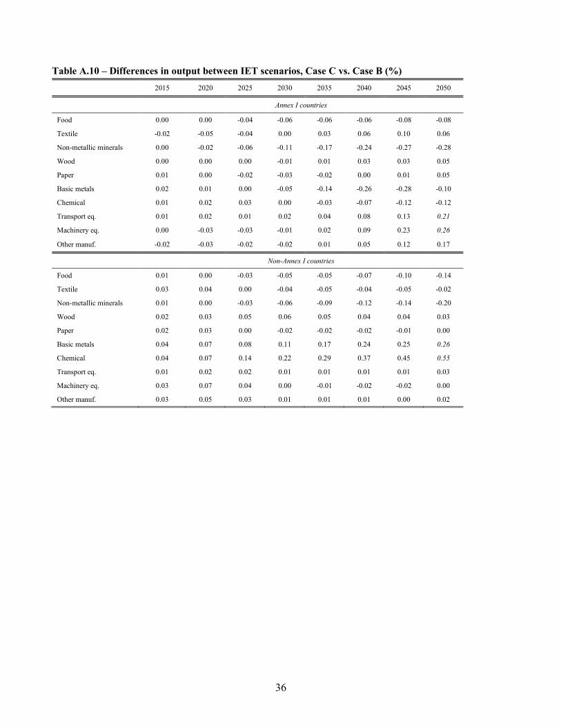
36

Table A.10 – Differences in output between IET scenarios, Case C vs. Case B (%)

2015 2020 2025 2030 2035 2040 2045 2050

Annex I countries

Food 0.00 0.00 -0.04 -0.06 -0.06 -0.06 -0.08 -0.08

Textile -0.02 -0.05 -0.04 0.00 0.03 0.06 0.10 0.06

Non-metallic minerals 0.00 -0.02 -0.06 -0.11 -0.17 -0.24 -0.27 -0.28

Wood 0.00 0.00 0.00 -0.01 0.01 0.03 0.03 0.05

Paper 0.01 0.00 -0.02 -0.03 -0.02 0.00 0.01 0.05

Basic metals 0.02 0.01 0.00 -0.05 -0.14 -0.26 -0.28 -0.10

Chemical 0.01 0.02 0.03 0.00 -0.03 -0.07 -0.12 -0.12

Transport eq. 0.01 0.02 0.01 0.02 0.04 0.08 0.13 0.21

Machinery eq. 0.00 -0.03 -0.03 -0.01 0.02 0.09 0.23 0.26

Other manuf. -0.02 -0.03 -0.02 -0.02 0.01 0.05 0.12 0.17

Non-Annex I countries

Food 0.01 0.00 -0.03 -0.05 -0.05 -0.07 -0.10 -0.14

Textile 0.03 0.04 0.00 -0.04 -0.05 -0.04 -0.05 -0.02

Non-metallic minerals 0.01 0.00 -0.03 -0.06 -0.09 -0.12 -0.14 -0.20

Wood 0.02 0.03 0.05 0.06 0.05 0.04 0.04 0.03

Paper 0.02 0.03 0.00 -0.02 -0.02 -0.02 -0.01 0.00

Basic metals 0.04 0.07 0.08 0.11 0.17 0.24 0.25 0.26

Chemical 0.04 0.07 0.14 0.22 0.29 0.37 0.45 0.55

Transport eq. 0.01 0.02 0.02 0.01 0.01 0.01 0.01 0.03

Machinery eq. 0.03 0.07 0.04 0.00 -0.01 -0.02 -0.02 0.00

Other manuf. 0.03 0.05 0.03 0.01 0.01 0.01 0.00 0.02