an analysis of the seasonal cycle and the business …1 introduction robert barsky and jeffrey...
TRANSCRIPT

Munich Personal RePEc Archive
An Analysis of the Seasonal Cycle and
the Business Cycle
Emara, Noha and Ma, Jinpeng
Rutgers University, Rutgers University
2019
Online at https://mpra.ub.uni-muenchen.de/99310/
MPRA Paper No. 99310, posted 30 Mar 2020 09:21 UTC

An Analysis of the Seasonal Cycle and the Business Cycle
Noha Emara∗ and Jinpeng Ma†
Abstract
Robert Barsky and Jeffrey Miron (1989) revealed the seasonal cycle of the U.S.
economy from 1948 to 1985 was characterized by a “bubble-like” expansion in the
second and fourth quarters, a “crash-like” contraction in the first quarter, and a mild
contraction in the third quarter. We replicate, in part, their seasonal cycle analysis
from 1946 to 2001. Our results are largely in line with theirs. Nonetheless, we find
the seasonal cycle is not stable and can evolve across time. In particular, the Great
Moderation affected both the business cycle and the seasonal cycle.
Robert Barsky and Jeffrey Miron also found real aggregates, like the output, move
together in the seasonal cycle across broadly defined sectors, similar to a phenomenon
observed under the conventional business cycle. They posed a challenge question
concerning why “the seasonal and the conventional business cycles are so similar.” To
answer their question, we focus on a number of aggregate variables with a recursive
application of the HP filter and find that aggregates, such as the GDP, consumption,
the S&P 500 Index, and so forth, have a “bubble-like” expansion and a “crash-like”
contraction in their cyclical trends in business cycle frequencies. Although preference
shifts and production synergy are the two major forces that drive the seasonal cycle,
we find the time-varying stochastic discount factor is the main cause of the business
cycle and plays a more important role in macroeconomic fluctuations in business cycle
frequencies than other factors.
JEL classification numbers: C53, C82, E24, E32, G12
Key words: Seasonal cycles, business cycles, jobless claims, unemployment rates,
labor productivity, GDP, S&P 500
∗Economics, Rutgers University, Camden, NJ, USA. E-mail: [email protected]†Economics, Rutgers University, Camden, NJ, USA. E-mail: [email protected]
1

1 Introduction
Robert Barsky and Jeffrey Miron (1989) provide a comprehensive analysis of seasonal
cycles for numerous aggregate variables for the U.S. economy from 1948 to 1985 and
discover that seasonal cycles have dominated short-term fluctuations of real economic
activities. Furthermore, they find that the seasonal cycle of the U.S. economy can be
characterized by a “bubble-like” expansion in the second and fourth quarters, a “crash-
like” contraction in the first quarter, and a mild contraction in the third quarter. An
intriguing result of theirs is that real aggregate variables, like the output, in the seasonal
cycle move together across broadly defined sectors, similar to a phenomenon observed
under the conventional business cycle. In their conclusion, they state, “The similarity
of the seasonal cycle and the business cycle presents a challenge because, to paraphrase
Lucas (1977, p. 10), ‘it suggests the possibility of a unified explanation’ of both business
cycles and seasonal cycles. By trying to understand precisely why the seasonal and the
conventional business cycles are so similar, we may be able to shed considerable light on
all aggregate fluctuations” (Robert Barsky and Jeffrey Miron 1989, p. 529).
Their findings and remark raise a question as to whether the seasonal cycle and the
business cycle have been driven by the same forces. If so, then one must explain why
the two cycles with different frequencies and periodic characterizations are found with the
same set of stylized facts in macroeconomic fluctuations. If not, then one must explain
why the seasonal cycle has been formed with a higher and fixed frequency of one cycle per
year while the business cycle has been formed with a lower and recurrent frequency. This
paper provides empirical evidence to resolve this difficulty with a recursive application of
the HP filter (Robert Hodrick and Edward Prescott 1997).
We agree with Robert Barsky and Jeffrey Miron that preference shifts and production
synergy are the two major forces behind the formation of the seasonal cycle. However,
these two forces are unlikely to be the causes for the business cycle. Our evidence has
been summarized in Figure 1, using the real GDP series. Figure 1a shows the seasonal
dummies estimated using their seasonal dummy model for the U.S. economy from 1946 to
2001.1 The seasonal cycle has a fixed frequency of one cycle per year, consistent with the
fact that preference shifts and production synergy at the seasonal frequency are probably
1The data are from BEA. Only seasonally adjusted data are available after 2001 because of a budget
cut.
2

associated with a shift in seasons in a calender year. These dummies represent quarterly
average deviations in output from the trend. The seasonal variations from 1946 to 2001,
after removal of the trend and the cyclical component, are shown in Figure 1d. The cyclical
trend shown in Figure 1b in business cycle frequencies is less regular than that shown in
Figure 1d but the patterns of bubble-like expansions and crash-like contractions are quite
similar.
-0.15
-0.1
-0.05
0
0.05
0.1
19
47
q1
19
48
q3
19
50
q1
19
51
q3
19
53
q1
19
54
q3
19
56
q1
19
57
q3
19
59
q1
19
60
q3
19
62
q1
19
63
q3
19
65
q1
19
66
q3
19
68
q1
19
69
q3
19
71
q1
19
72
q3
19
74
q1
19
75
q3
19
77
q1
19
78
q3
19
80
q1
19
81
q3
19
83
q1
19
84
q3
19
86
q1
19
87
q3
19
89
q1
19
90
q3
19
92
q1
19
93
q3
19
95
q1
19
96
q3
19
98
q1
19
99
q3
20
01
q1
Figure 1a. GDP Seasonal Dummies, 1947q1-2001q4
-0.05
-0.04
-0.03
-0.02
-0.01
0
0.01
0.02
0.03
0.04
19
47
q3
19
49
q3
19
51
q3
19
53
q3
19
55
q3
19
57
q3
19
59
q3
19
61
q3
19
63
q3
19
65
q3
19
67
q3
19
69
q3
19
71
q3
19
73
q3
19
75
q3
19
77
q3
19
79
q3
19
81
q3
19
83
q3
19
85
q3
19
87
q3
19
89
q3
19
91
q3
19
93
q3
19
95
q3
19
97
q3
19
99
q3
20
01
q3
20
03
q3
20
05
q3
20
07
q3
20
09
q3
20
11
q3
20
13
q3
Figure 1b. Cyclical Trend in Real GDP, 1947q1-2013q4
-0.03
-0.02
-0.01
0
0.01
0.02
19
47
q1
19
49
q1
19
51
q1
19
53
q1
19
55
q1
19
57
q1
19
59
q1
19
61
q1
19
63
q1
19
65
q1
19
67
q1
19
69
q1
19
71
q1
19
73
q1
19
75
q1
19
77
q1
19
79
q1
19
81
q1
19
83
q1
19
85
q1
19
87
q1
19
89
q1
19
91
q1
19
93
q1
19
95
q1
19
97
q1
19
99
q1
20
01
q1
20
03
q1
20
05
q1
20
07
q1
20
09
q1
20
11
q1
20
13
q1
Figure 1c. GDP Standard Browian Motion, H=0.5004, 1947q1-2013q4
-0.15
-0.1
-0.05
0
0.05
0.1
0.15
19
46
19
47
19
49
19
51
19
53
19
54
19
56
19
58
19
60
19
61
19
63
19
65
19
67
19
68
19
70
19
72
19
74
19
75
19
77
19
79
19
81
19
82
19
84
19
86
19
88
19
89
19
91
19
93
19
95
19
96
19
98
20
00
Figure 1d. GDP Seasonal Deviation from Trend, 1946-2001
In comparison with the cyclical trend in Figure 1b and the fractional Brownian motion
(fBm) in Figure 1c of the cyclical component, the seasonal dummies represent a larger
deviation from the trend than from the cyclical component. Such a conclusion is in line
3

with the findings of Robert Barsky and Jeffrey Miron about the dominance of the seasonal
cycle in short-term macroeconomic fluctuations. Our study of the seasonal cycle of other
aggregate variables appears in detail in Section 2. In particular, we present an analysis
of the seasonal pattern of various labor indicators, most of which were absent in Robert
Barsky and Jeffrey Miron but are very important lately to the monetary policy of the
Federal Reserve. We also find that the seasonal cycle is not stable and can evolve and
change with time. For example, the Great Moderation2 starting around 1985 affected both
the business cycle and the seasonal cycle.
We focus on the cyclical components of many real aggregates. We show that the cyclical
trends of many real aggregates have a bubble-like expansion and a crash-like contraction
in business cycle frequencies as well, a phenomenon similar to what has been observed in
the seasonal cycle in Figure 1d. We start with the cyclical component of the real GDP,
using the seasonally adjusted data from 1947 to 2013. We use the HP filter to remove
the trend in the GDP and then use it again numerous times to decompose the cyclical
component into two parts. One part constitutes the cyclical trend, Tc, shown in Figure 1b,
and the other part constitutes a fractional Brownian motion (fBm), shown in Figure 1c,
which has the Hurst parameter H ≈ 0.5,3 estimated by the first order quadratic variations
(Jacques Istas and Gabriel Lang 1997; Jean-Francois Coeurjolly 2001, 2008). The three
time series in Figures 1a, 1b, and 1c have a mean of zero and represent deviations from
the secular trend of the GDP.
Figures 1b and 1c both show that adversary shocks, fBm, and the endogenous weakness
in the cyclical trend, Tc, are the two major causes of a recession. The fBm part dipped into
2The Great Moderation, identified by Olivier Blanchard and John Simon (2001) (also see James Stock
and Mark Watson 2002 and references therein for detail), has affected not only the seasonal cycle, but also
the fBm of the GDP. The cyclical trend of the GDP is also affected but to a smaller degree. Alternatively,
one can also use the less volatile fBm of the GDP to explain the Great Moderation. See Table 6 in Section
3.3.1. for additional evidence.3Equivalently, Figure 1c is the noise component of the GDP that can be modeled with a fractional
ARIMA(p, d, q) process with d = 0 (Ton Dieker 2004). The real GDP and other aggregates, since WWII,
after removal of the secular or stochastic trend by the HP filter, follow an I(d) process with 1
2> d > 0.
We choose the equivalent fBm (H = 0.5) instead of a familiar ARIMA(p, d, q) process (d = 0) because
it is easier to estimate the single Hurst parameter H. An underlying assumption is that the zero-mean
cyclical component {Xt} as a stochastic process can be modeled by dXt
Xt
= σdBH
t , using the path-wise
stochastic integral, where BH
t is a fBm process with BH
0 = 0, 0 < H < 1. The model becomes the classical
Black-Scholes model when H = 0.5 and mean µ = 0.
4

the negative zone for each NBER recession (shown in shaded areas), indicating adversary
shocks occurred in the economy for each recession. However, an adversary shock is not a
sufficient condition for a recession. Adversary shocks were also observed during expansion
periods. More importantly, Figure 1b shows that, before each recession, the cyclical trend
started to lose its upward momentum and turned to a downward trend.
A unique feature of Figure 1b is that the cyclical trend of each expansion was quite
different from the others. Indeed, no two cyclical trends were the same for two adjacent
expansions. Such a difference arises likely from the difference in economic structures,
which were changed by a recession. For example, substantial differences exist before and
after the Great Recession in the housing and mortgage industries.
The two figures also show how a recession ends. A recession ends when the cyclical
trend makes a turn from a downward momentum into an upward momentum, with positive
shocks in fBm.4 Moreover, once the economy is in an upward trend, it persists for a lengthy
period, despite various adversary shocks. Nonetheless, because economic structures evolve
across time, the economic persistence differs for different economic structures. These
features together explain why the business cycle recurs in a lower frequency.
The cyclical trend in Figure 1b should be understood as a process of forming a bubble-
like expansion and a crash-like contraction in business cycle frequencies because the long-
term secular trend can be seen as the “equilibrium” of the economy, which is at mean
zero in Figure 1b. Such a process is similar to the excess volatility revealed by Robert
Shiller (1981) in the equity market, with the equilibrium indicated by the present value
of distributed dividends of a discounted model with constant discount rate. We provide a
study of the S&P 500 Index in Subsection 3.3. The S&P 500 has a cyclical trend similar to
Figure 1b of the GDP. Moreover, these bubble-like expansions and crash-like contractions
are commonly observed in the cyclical trends of many other aggregates. We may conclude
from them that macroeconomic fluctuations in the business cycle frequencies are, in fact,
the excess volatility of real economic activities. The force of the formation of such a process
shown in Figure 1b is likely because of the mean reverting around the secular trend. The
time-varying expected returns have been proved to be a major force behind the excess
volatility in equity (see, e.g., John Cochrane 2006). Thus, we also conduct a study of
4The only exception is the 2001 recession. We suspect the actual recession might have lasted longer
than what was declared by the NBER.
5

the cyclical trend in consumption in Subsection 3.4 and the stochastic discount factor
in Subsection 3.5. Through these studies, we have empirical evidence to show that the
intertemporal marginal rate of substitution or the stochastic discount factor has a time-
varying cyclical trend, with a pattern of bubbles and crashes around its conditional mean,
largely in relation to NBER recessions. We conclude from the patterns that the time-
varying stochastic discount factor is a major force causing macroeconomic fluctuations in
the business cycle frequencies, in line with the literature addressing excess volatility in the
equity market.
We are left to explain why the seasonal cycle and the business cycle share the same set
of stylized facts for macroeconomic fluctuations. The GDP is an aggregate variable. That
is, an upward trend, like a bubble-like expansion in the cyclical trend of the GDP, must
indicate that most sectors move in the same upward direction. Even though the downward
spikes of the cyclical trend in Figure 1b and the dips in the output in the component fBm
were uneven in the amplitudes across recessions, they had patterns similar to an output
drop in the first quarter of the seasonal cycle. The upward spikes of the cyclical trend
in Figure 1b is somewhat more complicated because the fBm part can be negative or
positive. This representation is, in fact, consistent with real economic activities where
economic growth during an expansion can lose momentum occasionally. Nevertheless, the
output across most sectors should also follow the cyclical trend described in Figure 1b and
the fBm in Figure 1c; otherwise it would be impossible for the GDP to display these same
patterns. These bubble-like spikes in the cyclical trend recur in lower frequencies than
in the seasonal cycle, but they are very similar to the bubble-like spikes in the second or
fourth quarter of the seasonal cycle, shown in Figures 1b and 1d.
To understand better the force that shapes the cyclical trend in Figure 1b, we further
decompose it into three forces. We find that the first difference of the cyclical trend has a
three-part decomposition:
(1−B)Tc = Component a + Component b + Component c
with Component c as the dominant force for (1 − B)Tc, where B is a backshift operator
with Bkxi = xi−k. The three-part decomposition of (1−B)Tc has been given in Figure 2.
This exercise indicates the cyclical trend Tc has been shaped by a major force c, to-
gether with two other minor forces, a and b. Interestingly, Component b leads Component
6
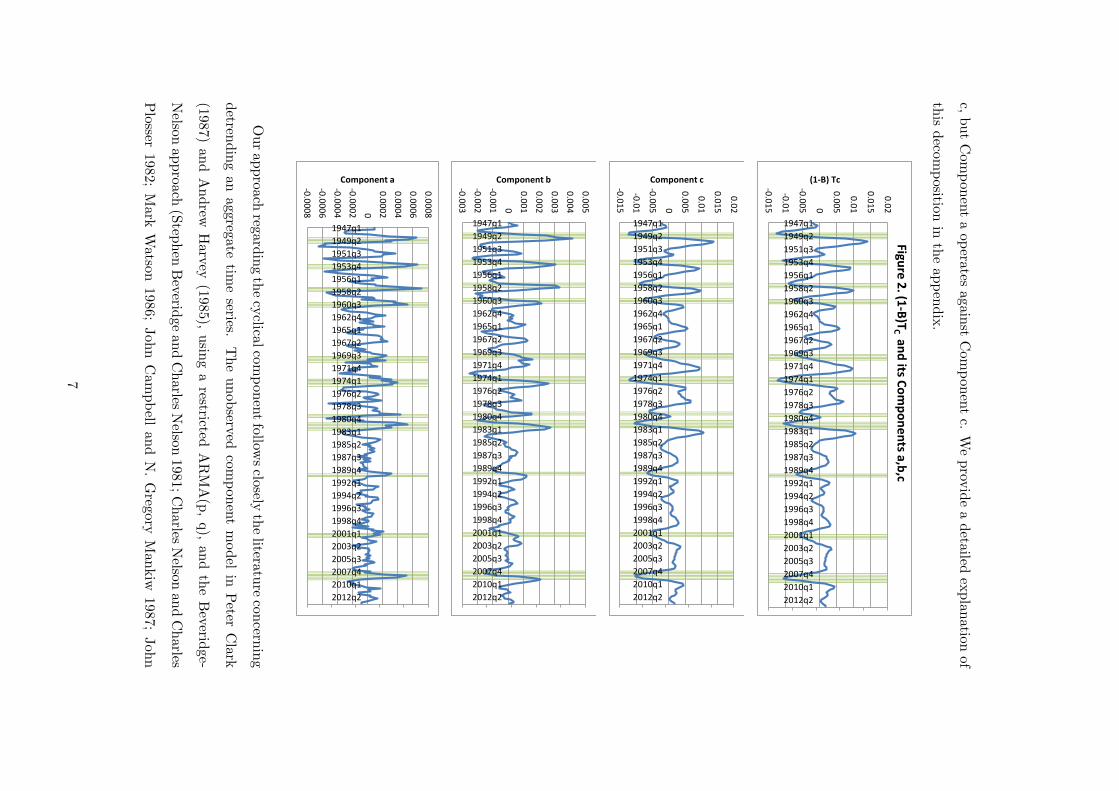
c,butCom
ponentaopera
tesagain
stCom
pon
entc.
Weprov
ideadetailed
explan
ationof
this
deco
mposition
intheappen
dix.
-0.0
15
-0.0
1
-0.0
05 0
0.0
05
0.0
1
0.0
15
0.0
21947q1
1949q2
1951q3
1953q4
1956q1
1958q2
1960q3
1962q4
1965q1
1967q2
1969q3
1971q4
1974q1
1976q2
1978q3
1980q4
1983q1
1985q2
1987q3
1989q4
1992q1
1994q2
1996q3
1998q4
2001q1
2003q2
2005q3
2007q4
2010q1
2012q2
(1-B) Tc
Fig
ure
2. (1
-B)T
C a
nd
its Co
mp
on
en
ts a,b
,c
-0.0
15
-0.0
1
-0.0
05 0
0.0
05
0.0
1
0.0
15
0.0
2
1947q1
1949q2
1951q3
1953q4
1956q1
1958q2
1960q3
1962q4
1965q1
1967q2
1969q3
1971q4
1974q1
1976q2
1978q3
1980q4
1983q1
1985q2
1987q3
1989q4
1992q1
1994q2
1996q3
1998q4
2001q1
2003q2
2005q3
2007q4
2010q1
2012q2
Component c
-0.0
03
-0.0
02
-0.0
01 0
0.0
01
0.0
02
0.0
03
0.0
04
0.0
05
1947q1
1949q2
1951q3
1953q4
1956q1
1958q2
1960q3
1962q4
1965q1
1967q2
1969q3
1971q4
1974q1
1976q2
1978q3
1980q4
1983q1
1985q2
1987q3
1989q4
1992q1
1994q2
1996q3
1998q4
2001q1
2003q2
2005q3
2007q4
2010q1
2012q2
Component b
-0.0
00
8
-0.0
00
6
-0.0
00
4
-0.0
00
2 0
0.0
00
2
0.0
00
4
0.0
00
6
0.0
00
8
1947q1
1949q2
1951q3
1953q4
1956q1
1958q2
1960q3
1962q4
1965q1
1967q2
1969q3
1971q4
1974q1
1976q2
1978q3
1980q4
1983q1
1985q2
1987q3
1989q4
1992q1
1994q2
1996q3
1998q4
2001q1
2003q2
2005q3
2007q4
2010q1
2012q2
Component a
Ourapproa
chreg
ardingthecyclica
lcom
pon
entfollow
sclosely
theliteratu
recon
cerning
detren
dingan
aggreg
ate
timeseries.
Theunob
servedcom
pon
entmodel
inPeter
Clark
(1987)andAndrew
Harvey
(1985),
usin
garestricted
ARMA(p,q),
andtheBeverid
ge-
Nelson
approach
(Step
hen
Beverid
geandCharles
Nelson
1981;Charles
Nelson
andCharles
Plosser
1982;
Mark
Watso
n198
6;JohnCam
pbell
andN.Gregory
Man
kiw
1987;Joh
n
7

Cochrane 1988), using a restriction-free ARMA(p, q), are most well known.5 A third
popular approach involves using the HP filter to decompose an aggregate time series into
a smooth trend and a cyclical component. Pierre Perron and Tatsuma Wada (2009)
provide a study of the three approaches and show that the HP filter can provide a trend
of the real GDP more smoothly than the other two.
The application of this HP filter in this paper differs in two major ways from those in
the literature. First, we find that the cyclical component of an aggregate such as the GDP
obtained from the HP filter is often not close to a “random walk.” Instead, it is quite
similar to a factional Brownian motion that has a long-range memory and persistence
or momentum trend, similar to that observed in Clive Granger (1980), Charles Nelson
and Charles Plosser 1982, Mark Watson 1986, John Campbell and N. Gregory Mankiw
1987, Francis Diebold and Glenn Rudebusch (1989), and Andrew Lo (1991), among others.
However, the long-range dependence that we address in this paper is in a business cycle
frequency, higher than the frequency of a secular trend.
In our estimation, many cyclical components (of the post war series) revealed after us-
ing the HP filter have a Hurst parameter H greater than 12 . For example, the cyclical com-
ponent of the GDP has H = 0.7965 after removal of the secular trend. That is, the cyclical
component of the HP filter itself contains a cyclical trend, displaying “intermediate-range”
dependence behavior. To separate this trend from the “noise” component at very high
frequencies, we apply the HP filter recursively to the cyclical components numerous times
so that the “noise” part eventually becomes an fBm with H close to 12 (H = 0.5004 for
the fBm in Figure 1c). Such an approach is largely motivated by John Cochrane (1988,
1991, 1994) and Robert King and Mark Watson (1994). John Cochrane (1988, 1991)
demonstrates that a time series with a unit root or a stationary series displaying near unit
root behavior contains a “small” random walk component. Robert King and Mark Wat-
son (1994) decompose the post-war unemployment and inflation series into three parts—a
secular trend (using a fixed low-pass filter), a business cycle trend (using a fixed band-pass
filter), and an irregular component (residuals after the two filters)—and establish a rela-
tionship between the two cyclical trends of unemployment and inflation in support of the
5See James Stock and Mark Watson (1988) for additional literature. Mark Watson (1986) shows that
the two approaches provide substantially different trends and cycles while James Morley, Charles Nelson,
and Eric Zivot (2003) reveal the essence causing these differences and provide a means of unifying the two
approaches. Also see Pierre Perron and Tatsuma Wada (2009) for a comparison study.
8
Phillips curve. John Cochrane (1994) uses the less volatile consumption as the trend and
the residual as the transitory component of GNP, using the VAR identification approach,
and finds the residual accounts for most variations in the GNP. He also establishes a similar
relationship between stock prices and dividends. Here, we use the HP filter recursively to
remove this “noise,” “irregular,” or transitory part from a number of aggregate variables.
The noise part is identified as the standard Brownian motion, which is known to be an
approximation of a random walk of i.i.d. random variables (with proper rescaling), under
the Donsker’s theorem (Tommi Sottinen 2001).
Second, our study is motivated by the remark of Robert Barsky and Jeffrey Miron. To
understand how different forces operate in recessions and expansions, we use the spline
approach to fit this cyclical trend of the cyclical component and decompose its first differ-
ence into three parts, as demonstrated in Figure 2. It appears that such a decomposition
is very fruitful. Many indicators thought to be lagging in the previous literature become
leading indicators. Thus, the approach extracts undisclosed information from these indi-
cators, possibly motivating many future studies of their implications for the seasonal cycle
and the business cycle.
The rest of this paper is organized as follows; Section 2 includes a detailed study of
the seasonal cycle, motivated by Robert Barsky and Jeffrey Miron. Section 3 addresses
the business cycle and focuses on the cyclical trends of various aggregate variables. In
particular, Section 3.5 documents the evidence that the stochastic discount factor also
has a pattern forming bubbles and crashes. Section 4 concludes the paper. The appendix
provides technical details of the approach used in the paper.
2 Seasonal Cycles
In this section we replicate, in part, a study of the seasonal cycle in Robert Barsky and
Jeffrey Miron (1989) using their seasonal dummies approach for the U.S. economy, with
the not seasonally adjusted data from 1946 to 2001. We follow Robert Barsky and Jeffrey
Miron in using the HP filter to remove the secular trend. Thus, the seasonal dummies we
obtain represent average deviations from the trends of the studied variables.
Our study focuses on the seasonal cycle of a number of real aggregate variables, such
as the GDP, consumption, investment, and so on. Our study differs from that of Robert
9

Barsky and Jeffrey Miron largely in that we find changes in the seasonal cycle over time,
partly because we have a larger sample size. Various former studies have tested a shift
of the seasonal cycle (Fabio Canova and Eric Ghysels 1994). The factors that cause such
a shift are not precisely known, but it appears the shift may be somehow related to the
average growth rates in the GDP and the volatility of the GDP. This possibility should
be investigated further because of its implication for the social welfare of economic policy
that aims at reducing seasonal or business cycle variations.
Let yk, k = 1, 2, · · · , N , be a time series. The HP filter uses the spline approach to
decompose the series into a smoothed (secular) trend {τk} and a cyclical component {ck},
that is, y = τ + c, by solving the following minimization problem
(HP ) min{τk}k=N
k=1{
N∑
k=1
(yk − τk)2 + λ
N−1∑
k=2
[(τk+1 − τk)− (τk − τk−1)]2},
where λ is a parameter that depends on whether the time series is quarterly or monthly
data. For a quarterly data series, λ is set at 1600 while it is set at 129600 for the monthly
data (Morten Ravn and Harald Uhlig 2001). For an aggregate variable investigated in this
paper, {yk} is the logarithm of the original series. The only exception is the unemployment
rate and labor productivity, where {yk} equals the original series.
2.1 Seasonal Fluctuations
The standard deviation of the deterministic seasonal component of output is estimated
at 4.35 percent deviation from the trend, which accounts for about 84.9 percent of the
deterministic fluctuations in output, as shown in Table 1. Similar magnitudes are shown
for gross investment, government spending, exports, and imports. As for consumption
spending, the standard deviation of the seasonal component is estimated at 6.15 percent
deviation from the trend and accounts for 90.8 percent of the deterministic fluctuations
in consumption. Similar magnitude is found for fixed investment where the standard
deviation of the deterministic seasonal component accounts for 8.37 percent deviation
from trend and for 84.6 percent of the deterministic fluctuations in fixed investment.
In line with Robert Barsky and Jeffrey Miron, the fluctuations of the deterministic
component of the seasonal dummies is at its highest for consumption spending on durable
goods and residential investment spending. As shown in the table, the standard devi-
ation of the seasonal dummies reaches 13.75 percent of deviations from the trend and
10

Table 1. Summary Statistics for Seasonal Dummies, 1946q1-2001q4
Standard Deviation Standard Error
Variables of Dummies of the Regression R-squared
Gross Domestic Product 0.0435 0.0184 0.849
Consumption 0.0615 0.0196 0.908
a. Durables 0.1375 0.0527 0.872
b. Services 0.0073 0.0090 0.400
Gross Investment 0.0308 0.0828 0.125
Fixed Investment 0.0837 0.0357 0.846
a. Nonresidential 0.0562 0.0390 0.676
Structures 0.0847 0.0385 0.830
b. Residential 0.1791 0.0603 0.899
Government 0.0400 0.0379 0.528
a. Federal 0.0419 0.0701 0.264
a. State and Local 0.0468 0.2004 0.846
Exports 0.0440 0.0557 0.387
Imports 0.0302 0.0490 0.278
Note-Average deviation from trend. Data source: Quarterly data from BEA.
accounts for 87.2 percent of the deterministic fluctuations in consumption spending on
durable goods. Similarly, the standard deviation of the seasonal component of residential
investment accounts for 17.91 percent of deviations from trend and accounts for almost
90 percent of its deterministic fluctuations. Furthermore, in line with Robert Barsky and
Jeffrey Miron, the deterministic component of the seasonal dummies for the consumption
spending on services is the smallest of all macroeconomic variables. For instance, the stan-
dard deviation of seasonal dummies for deviation from the trend in consumption spending
on services accounts for only 0.73 percent and explains about 40 percent of all variations.
11

Table 2. Summary Statistics for Seasonal Dummies, Various Periods
Periods⇒ 1946q1-1959q4 1960q1-1978q4 1979q1-2001q4
Standard Standard Standard Standard Standard Standard
Deviation Error of the Deviation Error of the Deviation Error of the
Variables ⇓ of Dummies Regression R-squared of Dummies Regression R-squared of Dummies Regression R-squared
Gross Domestic
Product 0.0566 0.0225 0.866 0.0481 0.0103 0.958 0.0341 0.0077 0.953
Consumption 0.0855 0.0185 0.957 0.0618 0.0112 0.970 0.0475 0.0083 0.972
a. Durables 0.1509 0.0752 0.806 0.1522 0.4187 0.933 0.1188 0.0343 0.926
b . Services 0.0075 0.0089 0.422 0.0098 0.0090 0.554 0.0080 0.0063 0.624
Gross Investment 0.0922 0.1118 0.421 0.0159 0.0621 0.065 0.0343 0.0435 0.395
Fixed Investment 0.1040 0.0495 0.820 0.0836 0.0278 0.905 0.0730 0.0233 0.911
a. Nonresidential 0.0820 0.0530 0.713 0.0511 0.0325 0.722 0.0468 0.0242 0.796
Structures 0.0862 0.0446 0.793 0.0909 0.0348 0.879 0.0794 0.0367 0.830
b. Residential 0.1682 0.0683 0.863 0.1910 0.0627 0.907 0.1772 0.0486 0.933
Government 0.0461 0.0532 0.433 0.0372 0.0246 0.707 0.0498 0.0194 0.873
a. Federal 0.0543 0.0801 0.324 0.0351 0.0443 0.398 0.0780 0.0455 0.754
b. State and Local 0.0673 0.0171 0.942 0.0478 0.0192 0.867 0.0340 0.0085 0.943
Exports 0.0610 0.0787 0.392 0.0592 0.0551 0.548 0.0218 0.0254 0.434
Imports 0.0171 0.0586 0.083 0.0443 0.0516 0.438 0.0323 0.0335 0.492
Note-Average deviation from trend. Data source: Quarterly data from BEA.
12

Table 2 expands the analysis of Table 1 by dividing the period from 1946:1-2001:4
into three periods such that period I covers 1946:1-1959:4, period II covers 1960:1-1978:4,
and period III covers 1979:1-2001:4. For the three periods, the standard deviation of the
deterministic seasonal component is the largest for consumption spending on durable goods
and fixed residential investment and is at the smallest for the consumption spending on
services. The standard deviation of the seasonal component for the government spending
is always less than 5 percent in the three periods and account for about 71 percent and
87 percent of the total fluctuations in government spending in the second and the third
periods, respectively, but only 43 percent in the first period.
Labor market is a focal point of the Federal Reserve. It is of a great interest to
investigate the seasonal patterns of various labor-related indicators. As shown in Table
3 the standard deviation of the deterministic seasonal component of the unemployment
rate is 7.15 percent of the deviation from trend, which accounts for about 65 percent of
the total deviations. The deterministic seasonal component of the hiring rate accounts for
the same percentage of total deviation, however its standard deviation is larger of about
21 percent of the deviations from trend. The deterministic seasonal component accounts
for the largest fluctuations in separation rate of about 91 percent of total fluctuations
with a standard deviation of about 16 percent deviations from trend, which is about three
quarters of 21 percent standard deviation of the hiring rate. Thus, substantial differences
exist between the seasonal components of the hiring rate and the separation rate. Our
study indicates that the hiring rate, similar to the unemployment rate, has been affected
more than the separation rate by the cyclical fluctuations.
As is obvious from the table, the deviations from trend of the weekly initial jobless
claims and the weekly continued jobless claims contain a larger stochastic component
than the other measures of the labor market discussed above. For instance, the standard
deviation of the deterministic seasonal component of the initial jobless claims is about
0.04 percent for the deviation from trend and it only explains 9.4 percent of the total
fluctuations. Also, the standard deviation of the deterministic seasonal component of the
continued jobless claims is about 2.1 percent and explains only about 15.5 percent of the
total fluctuations in this variable.
13

Table 3. Summary Statistics for Seasonal Dummies
Variable Standard Deviation Standard Error
of Dummies of the Regression R-squared
1948:01-2014:03
Unemployment Rate 0.0715 0.0521 0.649
Unemployment Level 0.0047 0.0035 0.639
2000:12-2014:01
Hire Rate 0.2056 0.1459 0.650
Separation Rate 0.1558 0.0467 0.912
1967:w1-2014:w52
Initial Jobless Claims 0.0378 0.1167 0.094
Continued Jobless Claims 0.0212 0.0490 0.155
Note-Average deviation from trend. Data source: Unemployment rate and level are NSA
monthly data from BLS. Hire and separation rates are NSA monthly data from BLS. Initial
and continued jobless data are NSA weekly data from the U.S. Department of Labor.
2.2 Seasonal Patterns
A more detailed investigation of the deterministic seasonal fluctuations is shown in
Table 4, where each macroeconomic variable is regressed on the seasonal dummies. Using
ordinary least squares (OLS), each macroeconomic variable is regressed on a set of quar-
terly seasonal dummies for the period from 1946:1 to 2001:4 and the three sub-periods.
As shown in the table, output for the whole period of 1946:1 to 2001:4 is well below
the trend in the first quarter and above the trend for the other three quarters, with a
smaller magnitude in the third quarter.6 A closer look at the pattern of output during
the three different periods shows that, not only the deviations from trend are similar to
the ones found for the whole period, but also the peaks of the deviations from the trend
are getting smaller as time goes on. For instance, the magnitude of the trough in the first
quarter was 9.4 percent, 7.4 percent, and 5.9 percent for the first, second, and third
6This result is different from the results of Robert Barsky and Jeffrey Miron for their shorter period
1948-1985, where output is shown to be, on average, well below the trend for the first quarter, slightly
below the trend in the second and third quarters, and well above the trend for the last quarter.
14

Table 4. Seasonal Variations of Seasonal Dummy Model, Various Periods
Periods⇒ 46-01 46-59 60-78 79-01
Variables⇓ Q1 Q2 Q3 Q4 Q1 Q2 Q3 Q4 Q1 Q2 Q3 Q4 Q1 Q2 Q3 Q4
Gross Domestic
Product -0.072 0.031 0.005 0.036 -0.094 0.025 0.015 0.056 -0.074 0.044 -0.011 0.041 -0.059 0.024 0.013 0.020
Consumption -0.097 0.041 -0.006 0.063 -0.133 0.049 -0.008 0.095 -0.097 0.048 -0.010 0.059 -0.077 0.030 -0.002 0.047
a. Durables -0.207 0.127 -0.037 0.122 -0.226 0.130 -0.033 0.147 -0.217 0.148 -0.066 0.137 -0.187 0.108 -0.016 0.093
b. Services 0.011 -0.010 -0.0004 -0.001 0.012 -0.0004 -0.001 -0.008 0.015 -0.012 -0.002 -0.002 0.006 -0.014 0.001 0.005
Gross
Investment 0.0001 -0.014 0.048 -0.035 0.050 -0.096 0.131 -0.070 -0.025 0.014 0.00004 0.015 -0.008 0.013 0.038 -0.055
Fixed
Investment -0.113 0.122 0.008 -0.013 -0.152 0.138 0.029 0.005 -0.106 0.127 0.003 -0.021 -0.097 0.107 -0.001 -0.017
a. Non-
residential -0.070 0.075 -0.032 0.030 -0.115 0.102 -0.023 0.052 -0.052 0.073 -0.043 0.025 -0.061 0.061 -0.029 0.022
Structures -0.131 0.093 0.052 -0.014 -0.136 0.082 0.065 -0.004 -0.141 0.102 0.049 -0.009 -0.119 0.091 0.046 -0.024
b. Residential -0.223 0.242 0.091 -0.106 -0.225 0.209 0.116 -0.071 -0.084 0.030 0.016 0.016 -0.211 0.247 0.074 -0.120
Government -0.059 0.040 0.031 -0.017 -0.084 0.030 0.017 0.016 -0.041 0.059 0.001 -0.120 -0.060 0.031 0.064 -0.034
a. Federal -0.069 0.029 0.037 -0.003 -0.090 0.004 -0.007 0.062 -0.028 0.058 -0.027 -0.005 -0.091 0.020 0.117 -0.041
a. State and
Local -0.053 0.057 0.035 -0.038 -0.072 0.080 0.054 -0.059 -0.055 0.062 0.030 -0.036 -0.039 0.040 0.027 -0.027
Exports -0.018 0.043 -0.063 0.039 -0.014 0.060 -0.091 0.053 -0.031 0.066 -0.080 0.047 -0.011 0.015 -0.032 0.024
Imports -0.014 0.059 -0.091 0.054 0.008 0.024 -0.006 -0.022 -0.023 0.069 0.003 -0.051 -0.045 0.045 0.007 -0.011
Note-Seasonal variations from the mean. Data source: Quarterly data from BEA
15

period, respectively. In addition, the magnitude of the peaks for the fourth quarter are
getting smaller as time goes on, as they reach 5.6 percent, 4.1 percent, and 2.0 percent for
the first, second, and the third periods, respectively.7
The components of output are generally procyclical with the exception of the consump-
tion expenditure on services. The deviations from the trend in consumption expenditure
on durable goods are, on average, below the trend in the first and third quarters but above
the trend in the second and fourth quarters. This indicates that durable goods generally
move with the trend deviations in output with the exception of the third quarter. In ad-
dition and in line with Robert Barsky and Jeffrey Miron, for all periods, the magnitudes
of these deviations are larger than that of output.
The trend deviations in residential investment are, on average, below the trend in the
first quarter, above the trend in the second and third quarters, and again below the trend
in the fourth quarter. The trend deviations for investment in structures are similar and
support Robert Barsky and Jeffrey Miron. Similarly, with few exceptions, trend deviations
in government spending and its two components, federal and state and local spending, on
average, are below the trend for the first and fourth quarters but above the trend for the
second and third quarters.
The deviations in export alternate between above and below the trend. For instance,
it is below the trend for the first and third quarters but above the trend in the second and
fourth quarters for the whole period from 1946-2011. As for imports, the trend deviations
for the whole period are very similar to those of exports, where, on average, the deviations
for the first and third quarters are below the trend but above the trend for the second and
fourth quarters. Seasonal patterns of export change lilttle with time, but those of import
do change with time.
Generally, the tendencies of output and its components are similar to the results of
Robert Barsky and Jeffrey Miron. More specifically, the decline in output from the fourth
to the first quarter is similar to the findings of Robert Barsky and Jeffrey Miron, which
is also reflected in almost all the components of output. In addition, our results confirm
the fourth quarter increase in consumption of durable goods and the first quarter peak in
7This result is different from the results of Robert Barsky and Jeffrey Miron for their shorter period
1948-1985, where output is shown to be, on average, well below the trend for the first quarter, slightly
below the trend in the second and third quarter, and well above the trend for the last quarter.
16
services spending rather than a first quarter decline. Further, we find a strong growth in
fixed investment in the second quarter followed by a slight increase in the third quarter and
slight decrease in the fourth quarter, that is, besides the increase in structures investment
in the second and third quarters. Finally, the peaks in federal and state and local spending
in the second and third quarters are all in agreement with the results of Robert Barsky and
Jeffrey Miron. These results seem to confirm that the trend deviations in macroeconomic
variables are correlated with the season and the weather: shopping season in the fourth
quarter results in an increase in spending, bad weather in the first quarter and the end of
the shopping season results in a drop in spending, and good weather in the second and
third quarters results in an increase in residential and structures spending. Changes in
season and weather appear to be two major forces driving preference shifts and production
synergy, a finding that supports Robert Barsky and Jeffrey Miron. A detailed discussion of
the two forces can be found further in Jeffrey Miron (1996). For a study of other developed
countries, see Joseph Beaulieu, Jeffrey MacKie-Mason and Jeffrey Miron (1992).
3 Business Cycles
We have presented our studies of the real GDP in Figures 1b, 1c, and 2. The methodol-
ogy of the study is addressed in the appendix. Here, we will document our studies of other
aggregate variables, such as the weekly continued claims for unemployment insurance, the
unemployment rate, labor productivity, the S&P 500 Index, and personal consumption ex-
penditures. We document the evidence that the patterns of the GDP shown in Figures 1b,
1c, and 2 are widely observed among these variables, especially in relation to recessions.
That is, we show that business cycle bubbles and crashes occur in these aggregate vari-
ables. These bubbles and crashes are less regular than the seasonal bubbles and crashes
and take a longer time to form. Despite the differences, these business cycle bubbles and
crashes are all similar. Moreover, they are similar to those observed in the seasonal cycle.
3.1 Weekly Continued Claims
The weekly initial and continued claims for unemployment insurance have lately re-
ceived more than usual attention among financial analysts and investors, partly because
the Federal Reserve watches these numbers closely, among other indicators, to determine
17

the strength of the U.S. labor market. In addition, its monetary policy is, in part, based
on the performance of these indicators. Quite surprisingly though, study or use of these
two weekly indicators for the business cycle among economists is quite rare. Margaret
McConnell (1998) is an exception. She studied the weekly initial claims and showed the
indicator provides useful information during a recession but fails to do so during an ex-
pansion. A jump in the initial claims during an expansion may not indicate the onset of a
recession. This fact limits the use of this indicator to forecast a recession even though it
sends out a correct signal after a recession has occurred. This present study is motivated
by her work as we investigate whether the weekly continued claims as an indicator are
useful in forecasting a recession. More importantly, by studying this indicator, we can
determine whether the indicator has a similar pattern in the cyclical trend of the GDP as
observed in Figure 1b.
First, we apply the HP filter to the logarithm time series of the NSA weekly continued
claim numbers and its seasonal factor8 from 1967:01:7 to 2014:03:15 to remove the secular
trend, with λ set at 33177600 (Morten Ravn and Harald Uhlig 2001). Second, we obtain the
cyclical time series, denoted {Jk}, by subtracting the cyclical component of the seasonal
factor from the cyclical component of the weekly continued claim numbers. Third, we
apply the HP filter again to {Jk} to get the stochastic trend, denoted {JSTk}, and the
cyclical component, denoted {Jk − JSTk}, which is decomposed further into a cyclical
trend {JCTk} and its fBm component {JCk}, which has the Hurst parameter H = 0.4969,
estimated using Patrick Flandrin’s (1992) method by computing the slope of the log-log
plot of the variance versus the level.
Figure 3 documents these exercises. Figure 3a presents the cyclical trend series {JCTk}
and Figure 3b presents the stochastic trend {JSTk}, with the fBm given in Figure 3c.
These figures represent the cyclical deviation from the secular trend, after adjustment for
the seasonal factor. The time series JST is a leading indicator, and it starts to turn
upward before a recession begins. However, both JCT and JST are lagging indicators
for predicting the end of a recession. Without JST , JCT may provide a false signal, a
8The seasonal factor (SF) is determined by the beginning of the year and fixed for the whole year. It
is typically modified in March. See William Cleveland and Stuart Scott (2007) for a detailed analysis of
how the seasonal factor is determined. The cyclical deviation of the weekly continued claims is adjusted
with the SF in this paper.
18

case similar to that documented by Margaret McConnell (1998) for the initial claims.9
With the help of JST , JCT can provide a better timed signal of a recession. The fBm
component is a reliable indicator for forecasting the end of a recession.
-0.15
-0.1
-0.05
0
0.05
0.1
0.15
1/7
/19
67
1/7
/19
69
1/7
/19
71
1/7
/19
73
1/7
/19
75
1/7
/19
77
1/7
/19
79
1/7
/19
81
1/7
/19
83
1/7
/19
85
1/7
/19
87
1/7
/19
89
1/7
/19
91
1/7
/19
93
1/7
/19
95
1/7
/19
97
1/7
/19
99
1/7
/20
01
1/7
/20
03
1/7
/20
05
1/7
/20
07
1/7
/20
09
1/7
/20
11
1/7
/20
13
Figure 3a. Cyclical Trend JCT, 1967-2013
-0.1
-0.08
-0.06
-0.04
-0.02
0
0.02
0.04
0.06
0.08
1/7
/19
67
1/7
/19
69
1/7
/19
71
1/7
/19
73
1/7
/19
75
1/7
/19
77
1/7
/19
79
1/7
/19
81
1/7
/19
83
1/7
/19
85
1/7
/19
87
1/7
/19
89
1/7
/19
91
1/7
/19
93
1/7
/19
95
1/7
/19
97
1/7
/19
99
1/7
/20
01
1/7
/20
03
1/7
/20
05
1/7
/20
07
1/7
/20
09
1/7
/20
11
1/7
/20
13
Figure 3b. Stochastic Trend JST, 1967-2013
-0.3
-0.2
-0.1
0
0.1
0.2
0.3
0.4
0.5
1/7
/19
67
1/7
/19
69
1/7
/19
71
1/7
/19
73
1/7
/19
75
1/7
/19
77
1/7
/19
79
1/7
/19
81
1/7
/19
83
1/7
/19
85
1/7
/19
87
1/7
/19
89
1/7
/19
91
1/7
/19
93
1/7
/19
95
1/7
/19
97
1/7
/19
99
1/7
/20
01
1/7
/20
03
1/7
/20
05
1/7
/20
07
1/7
/20
09
1/7
/20
11
1/7
/20
13
Figure 3c. fBm Component, H=0.4969, 1967-2013
These figures reveal some important causes for a recession. They should shed consid-
erable light on how recessions begin and end. First, if a recession is caused only by shocks,
then one should not be able to observe the turn in JCT and JST before a recession begins.
9The analysis for this indicator is available upon request.
19

Because these two indicators lead a recession, far before a recession begins, the economy
starts to lose its momentum, as shown in Figure 1b. This loss in momentum makes the
economy fragile to external shocks. Second, during a recession, the fBm component can
spike much higher. Many firms lay off workers in massive numbers during a recession.
However, once such layoffs taper off, as fBm indicates, a recession ends. The turn in fBm
is sharp and reliable. This may indicate why a recession is typically shorter than an ex-
pansion, and there is asymmetry in the business cycle, similar to that found in a number of
papers on Friedman’s plucking model (Milton Friedman 1993; Francisco Nadal De Simone
and Sean Clarke 2007; Tingguo Zheng, Yujuan Teng, and Tao Song 2010). However, our
results show that it is far from conclusive that the plucking caused by a transitory shock,
as stated in these papers, is indeed the only cause of a recession.
As observed above, JST and JCT lag to predict the end of a recession. Such an
issue can be overcome by extracting more signals from them after decomposing them into
different components:
(1−B)JST = JST ′s Components a +b+ c
(1−B)JCT = JCT ’s Components a +b+ c
The results are shown in Figures 4 and 5. Because Component c in both cases is domi-
nant, we have (1−B)JST ≃ JST ’s Component c and (1−B)JCT ≃ JCT ’s Component c,
(Components c are not reported in the two figures.) The dominance of Component c does
not mean that Components a and b are not important. In fact, they provide very impor-
tant information about business cycles, especially with respect to recessions.
Figures 4 and 5 also show that the cyclical patterns revealed here should come from
the data, not from the HP filter, which is often criticized as generating spurious cycles.
No randomly generated data can produce such a nice pattern in Figures 4 and 5 under
the HP filter.10
10Simulation results are out of the scope and not reported here.
20

-0.0
01
5
-0.0
01
-0.0
00
5 0
0.0
00
5
0.0
01
0.0
01
5
1/7/1967
1/7/1969
1/7/1971
1/7/1973
1/7/1975
1/7/1977
1/7/1979
1/7/1981
1/7/1983
1/7/1985
1/7/1987
1/7/1989
1/7/1991
1/7/1993
1/7/1995
1/7/1997
1/7/1999
1/7/2001
1/7/2003
1/7/2005
1/7/2007
1/7/2009
1/7/2011
1/7/2013
(1-B)JST
Fig
ure
4. (1-B
) JST
an
d its C
om
po
ne
nts a
, b, c, 1
96
7-2
01
3
-8E
-08
-6E
-08
-4E
-08
-2E
-08 0
2E
-08
4E
-08
6E
-08
Component a
-0.0
00
01
5
-0.0
00
01
-0.0
00
00
5 0
0.0
00
00
5
0.0
00
01
Component b
21

-0.002
-0.0015
-0.001
-0.0005
0
0.0005
0.001
0.0015
0.002
0.0025
1/7
/19
67
1/7
/19
69
1/7
/19
71
1/7
/19
73
1/7
/19
75
1/7
/19
77
1/7
/19
79
1/7
/19
81
1/7
/19
83
1/7
/19
85
1/7
/19
87
1/7
/19
89
1/7
/19
91
1/7
/19
93
1/7
/19
95
1/7
/19
97
1/7
/19
99
1/7
/20
01
1/7
/20
03
1/7
/20
05
1/7
/20
07
1/7
/20
09
1/7
/20
11
1/7
/20
13(1
-B)J
CT
Figure 5. (1-B) JCT and its Components a, b, c, 1967-2013
-3E-07
-2.5E-07
-2E-07
-1.5E-07
-1E-07
-5E-08
0
5E-08
0.0000001
1.5E-07
0.0000002
Co
mp
on
en
t a
-0.000025
-0.00002
-0.000015
-0.00001
-0.000005
0
0.000005
0.00001
0.000015
0.00002
0.000025
Co
mp
on
en
t b
As shown in Figures 4 and 5, Component b is a leading indicator in predicting the
beginning of a recession. Note that Component a operates against Component c. Thus,
both Components c and a become leading indicators in predicting the end of recessions.
(1−B)JST and (1−B)JCT are leading indicators as well. They reach their local peaks
before the end of recessions. Two “false” signals around 1987 and 1996 with respect to
22

the NBER recessions occur using (1 − B)JST and (1 − B)JCT .11 Such an issue can be
eliminated by using JST .
We can conclude from Figures 3, 4 and 5 that excess volatility exists in the cyclical
trend of the continued claims numbers.
3.2 Unemployment Rate and Labor Productivity
The unemployment rate and labor productivity are the two most important measures
for the labor market. Numerous articles have been written on these indicators. The
following summarizes our understanding of the unemployment rate as leading economists
describe it:
The unemployment rate is a trendless indicator that moves in the opposite
direction from most other cyclical indicators. [...] The NBER business-cycle
chronology considers economic activity, which grows along an upward trend.
As a result, the unemployment rate often rises before the peak of economic
activity, when activity is still rising but below its normal trend rate of increase.
Thus, the unemployment rate is often a leading indicator of the business-cycle
peak. [...] On the other hand, the unemployment rate often continues to rise
after activity has reached its trough. In this respect, the unemployment rate
is a lagging indicator. (http://nber.org/cycles/recessions_faq.html)
Nonetheless, controversies abound concerning these two indicators. For example, to
answer the question as to why the Phillips curve and the Beveridge curve models have
both lost their forecasting capability recently, Alan Krueger, Judd Cramer, and David
Cho (2014) declared that the existing unemployment rate is an insufficient indicator and
does not reflect well the current strength or weakness of the labor market. A solution
suggested by these authors is to replace the existing one with the unemployment rate for
workers unemployed for less than 26 weeks. Such an alternative would fail to account for
a great number of unemployed workers, those unemployed for durations longer than 26
weeks. The authors claimed that these workers are on the margins and become irrelevant
11There was some truth behind the two “false” signals if one recalled the two minicrashes in equity market
in these years. Many still question the two crashes because they were not supported by the fundamentals, an
understanding our figures contradict. Fundamentals did show substantial weakness during the minicrashes.
23

for increasing wages. A question left unanswered is the cause of the sharply increasing
long-term unemployment rate, especially from the Great Recession.
Labor productivity is procyclical: it is higher during booms and lower during slumps
(Susanto Basu and John Fernald 2001). However, Ellen McGrattan and Edward Prescott
(2012) provide a new puzzle: Measured in level, labor productivity is procyclical and
positively correlated with the GDP by 54% for the period from 1960 to 1985; since then,
it has become much less procyclical, and its correlation with the GDP has dramatically
dropped to only 5% (see Figure 1 in Ellen McGrattan and Edward Prescott 2012).
Motivated by these studies and Robert Barsky and Jeffrey Miron (1989), we investigate
how these two indicators perform in relation to the business cycle and whether similar
business cycle bubble and crash spikes conform with those observed in the GDP and the
continued claim numbers. Labor productivity in our paper is measured by percentage
change from previous of the output per hour for business sectors, downloaded from BLS.
We use the rate of labor productivity rather than the level because we want to compare
it with the unemployment rate.
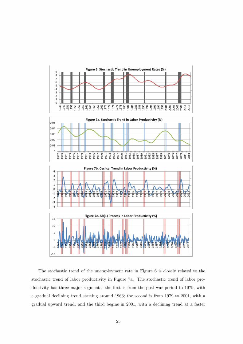
Our procedure is as follows. First, we apply the HP filter, as in Ellen McGrattan and
Edward Prescott (2012), to obtain the stochastic trends12 of the two indicators (without
taking the logarithm). These stochastic trends represent the trends over long-term hori-
zons. Figure 6 shows the stochastic trend UST for the unemployment rate, and Figure 7a
shows the stochastic trend for labor productivity. Second, we apply the HP filter to the
cyclical part of labor productivity recursively13 and decompose labor productivity into a
cyclical trend component (Figure 7b) and an AR(1) process (Figure 7c and Table 5).
Our decompositions are given as follows:
Unemployment rate = UST in Figure 6 + CU in Figure 8
Labor productivity = Figure 7a + Figures 7b +AR(1) in Figure 7c
12The two indicators have no secular trends.13The exact number is 100 times. However, one can choose other numbers near 100 without changing
the essence of what we intend to obtain from the cyclical trend.
24
0
1
2
3
4
5
6
7
8
9
19
48
19
49
19
51
19
53
19
55
19
57
19
59
19
61
19
63
19
65
19
67
19
69
19
71
19
72
19
74
19
76
19
78
19
80
19
82
19
84
19
86
19
88
19
90
19
92
19
94
19
95
19
97
19
99
20
01
20
03
20
05
20
07
20
09
20
11
20
13
Figure 6. Stochastic Trend in Unemployment Rates (%)
0
0.01
0.02
0.03
0.04
0.05
19
47
19
49
19
51
19
53
19
55
19
57
19
59
19
61
19
63
19
65
19
67
19
69
19
71
19
73
19
75
19
77
19
79
19
81
19
83
19
85
19
87
19
89
19
91
19
93
19
95
19
97
19
99
20
01
20
03
20
05
20
07
20
09
20
11
20
13
Figure 7a. Stochastic Trend in Labor Productivity (%)
-4
-3
-2
-1
0
1
2
3
4
19
47
19
49
19
51
19
53
19
55
19
57
19
59
19
61
19
63
19
65
19
67
19
69
19
71
19
73
19
75
19
77
19
79
19
81
19
83
19
85
19
87
19
89
19
91
19
93
19
95
19
97
19
99
20
01
20
03
20
05
20
07
20
09
20
11
20
13
Figure 7b. Cyclical Trend in Labor Productivity (%)
-10
-5
0
5
10
15
19
47
19
49
19
51
19
53
19
55
19
57
19
59
19
61
19
63
19
65
19
67
19
69
19
71
19
73
19
75
19
77
19
79
19
81
19
83
19
85
19
87
19
89
19
91
19
93
19
95
19
97
19
99
20
01
20
03
20
05
20
07
20
09
20
11
20
13
Figure 7c. AR(1) Process in Labor Productivity (%)
The stochastic trend of the unemployment rate in Figure 6 is closely related to the
stochastic trend of labor productivity in Figure 7a. The stochastic trend of labor pro-
ductivity has three major segments: the first is from the post-war period to 1979, with
a gradual declining trend starting around 1963; the second is from 1979 to 2001, with a
gradual upward trend; and the third begins in 2001, with a declining trend at a faster
25

Table 5. AR(1) process of labor productivity
Conditional Probability Distribution: Gaussian Standard t
Parameter Value Error Statistic
Constant -1.9089e-05 0.19045 -0.0001
AR(1) -0.263626 0.056552 -4.6617
Variance 8.74395 0.687041 12.727
declining pace than the decline in the 1970s. The end of the third declining trend has
not been shown, but it will probably end at next recession. A good sign is that the long
term unemployment trend starts to show a down turn, which is often accompanied with
an upward trend in long-term labor productivity.
The stochastic trend of the unemployment rate also has three major periods: the first
is from the post-war period to 1982, with a gradual uptrend, increasing from the lowest
point, 4 percent, in 1952 and 1967 to more than 8 percent in 1982. In addition, in this
period long-term labor productivity shows a declining trend. The second is from 1982 to
1999, with a downward trend. The long-term unemployment rate declined from more than
8 percent to about 4.5 percent. This period had surging long-term labor productivity. The
unemployment rate surged from the low of 4.5 percent in 1999 to more than 8 percent
again in 2011. This period also had a sharp decline in long-term labor productivity.
The reason long-term labor productivity affects the long-term unemployment rate may be
quite obvious: Higher labor productivity increases the demand for labor. What is not so
clear is the relationship between the declining trend in the long-term unemployment rate
and the volatility in the cyclical trend and the AR(1) process of labor productivity. The
two periods of 1961-1968 and 1982-1999 both have a downward trend in the long-term
unemployment rates. Figures 7b and 7c show the cyclical trends and the AR(1) processes
of labor productivity for both periods have lower volatilities than other periods have.
The Great Moderation, starting around 1985 (Olivier Blanchard and John Simon 2001;
James Stock and Mark Watson 2002), affected the seasonal cycle and the business cycle.
James Stock and Mark Watson (2002) provided many causes for the Great Moderation.
The lower volatility identified above indicates the Great Moderation should have something
to do with the declining trend in the long-term unemployment rate and the uptrend in
long-term labor productivity.
26

Joseph Beaulieu, Jeffrey MacKie-Mason, and Jeffrey Miron (1992) found an economy
with a large seasonal cycle also has a large business cycle. In our study of the seasonal
cycle in Section 2, we divided the U.S. economy into three subperiods. We can now see
from Figure 1 to 7 the same phenomenon as observed by Joseph Beaulieu, Jeffrey MacKie-
Mason, and Jeffrey Miron. A subperiod that has a large seasonal cycle also has a large
business cycle (see Table 6 below). Moreover, such a phenomenon is related to the fact that
long-term labor productivity is in a declining trend and the long-term unemployment rate
is in an upward trend. This phenomenon may explain why the Great Recession happened
in 2008, when the long-term unemployment rate was near its peak. At another point
in the 1980s, that recession was the worst since the Great Depression. In another words,
these two worst recessions since World War II occurred when long-term labor productivity
was near its lowest point and the long-term unemployment rate was near its peak. This
phenomenon might be explained as follows: First, when long-term labor productivity is
near the lowest point, there must exist more workers who have lost their skills. Second,
when long-term labor productivity is in a declining trend, it should be harder for firms
to raise labor productivity during a recession because it is going against the trend. Thus,
firms may need to lay off more workers at such points to raise labor productivity.
Considering all eleven recessions, long-term labor productivity (Figure 7b) declined in
only one, in 1954, when long-term labor productivity was in a downtrend. For the other
recessions, long-term labor productivity either remained flat or moved higher, indicating
a recession is helpful for raising long-term labor productivity. The recessionary effect on
labor productivity can be seen in the cyclical trend shown in Figure 7b as well. During
recessions, cyclical labor productivity is higher.
Whether the level of labor productivity (output per hour) is procyclical depends on
whether the AR(1) process and the cyclical trend stay in the positive zone during expan-
sions and in the negative zone during recessions. As shown in Figure 7c, labor productivity
in the AR(1) component declined rather sharply into negative zones during recession pe-
riods. Interestingly enough, by the end of each recession, a surge in labor productivity
to the positive occurs even during the AR(1) process. One key observation here is that,
before a recession, there is a substantial decline, often into the negative zone, in the cycli-
cal trend of labor productivity. These observations support our claim that recessions are
likely caused by firms’ demands to overcome declining cyclical labor productivity. Iron-
27

ically, such a practice will cause a decline in labor productivity in the AR(1) part first.
Thus, asserting the level of labor productivity is procyclical is not very precise considering
the evolution of labor productivity during recessions and expansions.
Our analysis appears to be consistent with the idea of creative destruction initiated by
Joseph Schumpeter (1942) and further developed by Philippe Aghion and Peter Howitt
(1992). However, creative destruction can go well beyond innovations in technology and
formation of human capital. For example, it can extend to other important aspects of the
economy, such as firm-customer relationships (Erik Canton and Harald Uhlig 1999).
Table 8 in Subsection 3.3.1 shows that labor productivity is negatively related to the
GDP and consumption in the cyclical trend by two unexpected large numbers, -0.556
and -0.387, respectively, for the period from 1950 to 2013, and the correlations remain
steady for the period from 1950 to 1985. The negative relationships are even higher for
the period from 1986 to 2013. The negative relation arises because labor productivity
increases in the cyclical trend during recession periods and starts to fall after a recession
(Figure 7b). This feature shows that a recession is a period in which firms use layoffs of
less productive workers to battle falling productivity. Massive layoffs across broad sectors
send the economy into a recession. The sharp increases in the continued claim numbers
during recessions appear to support such a theory. Thus, the force behind a recession is
very different from the seasonal cycle, in which labor productivity in the seasonal cycle
has been found procyclical by Robert Barsky and Jeffrey Miron (1989) and Jeffrey Miron
(1996).
We find that the relationship between labor productivity (measured in percent change)
and the GDP or consumption does not change substantially for the two different periods
of 1950-1985 and 1986-2013, in contrast to what has been documented in Ellen McGrattan
and Edward Prescott (2012). The lower volatility in the AR(1) of labor productivity for
the period 1986-2013 is likely affected by the Great Moderation.
As with the GDP, we can decompose the first differencing (1−B)UST of the stochastic
trend UST for the unemployment rate into three components:
(1−B)UST = UST’s Components a+ b+ c.
The result is shown in Figure 8a, together with the cyclical unemployment rate (CU) in
Figure 8b, which is obtained by removing UST from the original unemployment rate time
series. From Figure 8a, we can see that Component b is a leading indicator in predicting
28

the beginning of a recession while Component a is a reliable leading indicator in predicting
the end of a recession. The cyclical component (CU) of Figure 8b is also a reliable indicator
of recessions. These observations provide some new understanding of the unemployment
rate.
-0.06
-0.04
-0.02
0
0.02
0.04
0.06
0.08
0.1
19
48
19
50
19
52
19
54
19
56
19
58
19
60
19
62
19
64
19
66
19
68
19
71
19
73
19
75
19
77
19
79
19
81
19
83
19
85
19
87
19
89
19
91
19
93
19
96
19
98
20
00
20
02
20
04
20
06
20
08
20
10
20
12
Co
mp
on
en
t C
of
(1-B
)US
T
Figure 8a. Component C of (1-B)UST, 1948-2013
-0.002
-0.0015
-0.001
-0.0005
0
0.0005
0.001
0.0015
Co
mp
on
en
t b
of
(1-b
)US
T
-0.00005
-0.00004
-0.00003
-0.00002
-0.00001
0
0.00001
0.00002
0.00003
Co
mp
on
en
t a
of
(1-B
)US
T
-2
-1
0
1
2
3
4
19
48
19
50
19
52
19
54
19
56
19
58
19
60
19
62
19
64
19
66
19
68
19
71
19
73
19
75
19
77
19
79
19
81
19
83
19
85
19
87
19
89
19
91
19
93
19
96
19
98
20
00
20
02
20
04
20
06
20
08
20
10
20
12
Cy
clic
al
Co
mp
on
en
t C
U(%
)
Figure 8b. Cyclical Component CU(%)
29

3.3 S&P 500 Index
The efficient market hypothesis claims that the equity market follows the fundamentals
of the economy. It may deviate from the fundamentals occasionally but not for a very
long period. That is, the equity market must be closely affected by the business cycle.
In particular, the expected returns should be lower during an economic boom and higher
during an economic slump. Thus, the equity market should move higher during booms
and lower during slumps. On the other hand, the excess volatility discovered by Robert
Shiller (1981) shows that the equity market, using the real S&P 500 Index as a proxy, may
often form a bubble (or crash), with prices that are well above (or below) a level supported
by the fundamentals in real terms. The formation of a bubble or crash in Shiller (1981)
takes a longer time than a typical business cycle duration. Robert Shiller (1981) uses the
present value of distributed dividends as the level supported by the fundamentals adjusted
by the inflation. Even though Robert Shiller (1981) does not provide a precise time when a
bubble or crash is formed in an equity market, a juncture of the efficient market hypothesis
and his excess volatility indicates that a bubble should be formed more often during an
economic boom and a crash should be formed more often during an economic slump.14
In this section, we provide a study of the S&P 500 Index quarterly close prices adjusted
with dividends from 1950Q1 to 2014Q2. The data were downloaded from Yahoo. We use
the same methodology as was used to analyze the GDP data. Figure 9 shows the cyclical
trend SPT and the fBm of the S&P 500 Index in such an exercise. Figure 9a shows the
efficient market hypothesis, in fact, holds very well in the sense that those price spikes
near recessions of the cyclical trend of the S&P 500 are very much like those in the GDP
shown in Figure 1b.
The bubbles and crashes shown in Figure 9a arise from the deviations from the secular
trend while Robert Shiller (1981) identifies a bubble or crash as deviations from the fun-
damentals computed by a discounted model with a constant discount rate. Our bubbles
and crashes appear to be much smaller in amplitude and occur more often than those
14This explanation does not mean that the equity market will not form a bubble or crash at other
times. For example, Black Monday, October 19, 1987, and a minicrash that occurred on Friday, October
13, 1989, were both mysterious. These two minicrashes occurred when the economy was in an NBER
expansion. Nonetheless, the weakness in the GDP during these two periods, which Figure 1 shows, may
have contributed to these two minicrashes.
30

identified by Shiller. That is, a major bubble or crash (in annual data) in Shiller consists
of a sequence of bubbles or crashes (in quarterly or monthly data) identified in this paper.
-0.3
-0.25
-0.2
-0.15
-0.1
-0.05
0
0.05
0.1
0.15
0.2
0.25
19
50
q2
19
52
q2
19
54
q2
19
56
q2
19
58
q2
19
60
q2
19
62
q2
19
64
q2
19
66
q2
19
68
q2
19
70
q2
19
72
q2
19
74
q2
19
76
q2
19
78
q2
19
80
q2
19
82
q2
19
84
q2
19
86
q2
19
88
q2
19
90
q2
19
92
q2
19
94
q2
19
96
q2
19
98
q2
20
00
q2
20
02
q2
20
04
q2
20
06
q2
20
08
q2
20
10
q2
20
12
q2
S&
P 5
00
Cy
clic
al
Tre
nd
Figure 9a. S&P 500 Cyclical Trend SPT, 1950q2-2014q2
-0.25
-0.2
-0.15
-0.1
-0.05
0
0.05
0.1
0.15
0.2
S&
P 5
00
fB
m
Figure 9b. S&P 500 fBm, H=0.5058
3.3.1 Key Statistics
We provide some key statistics in tables in this section. Two types of excess volatility
occur in the cyclical trend and the fBm of the S&P 500. The first is based on Figure 9a in
which the cyclical trend of the Index deviates from its secular trend to form bubbles and
crashes. These bubbles and crashes are similar to those observed in real aggregates, such
as the GDP, the unemployment rate, and so on. The standard deviations of the cyclical
trend of the S&P 500 reached about 16 percent for the period of 1950q1-2001q4 while the
standard deviations of the fBm were about 10 percent. The standard deviations of the
cyclical trend and the fBm of the Index were the highest in the period from 1960q1 to
31

1978q4. The Great Moderation seems to affect excess volatility of the S&P 500.
The second is the difference in the standard deviations of the S&p 500 from those of
the GDP, consumption, and other aggregates. The cyclical trend of the S&P 500 appears
to have cycles with much larger amplitudes, as shown in Tables 6 and 7. For instance, the
standard deviation of the cyclical trend of the GDP over the period 1947:q1 to 2001:q4
reached only 3% while that of the S&P 500 reached about 16 percent over roughly the
same period. Furthermore, the period from 1960:q1 to 1978:q4 had the largest gap between
the standard deviations of these two variables and accounted for 20.3 percent with the
S&P 500 superseding the GDP. The first type of excess volatility is closely related to the
original finding in Robert Shiller (1981) while the second is more related to the equity
premium puzzle in Rajnish Mehra and Edward Prescott (1985).
Table 8 shows the correlation between various aggregate variables in the periods 1950-
2013, 1950-1985, and 1986-2013. This table reveals that the fBm component of the S&P
500 is positively related to those in the GDP and consumption, but the magnitudes of
correlation are very small.15 That is, the HP filter extracted much information from the
original data in terms of the cyclical trends. The cyclical trend of the S&P 500 is positively
related to the cyclical trends in the GDP and consumption by about 50 percent and the
correlation becomes higher for the period of 1986-2013. Thus, volatility in the noise part
of the equity market does not follow that in the fundamentals of the economy, especially
during the period 1950-1985. That is, different forces drive the noise parts of the equity
market and the real economy. We conclude that the data in Tables 7 and 8 support
Shiller’s excess volatility (also see Table 9) in both the short and the long terms.
The low correlation at about 20 percent between the equity market and the macroe-
conomic aggregates, such as the GDP and consumption, has been called the correlation
puzzle (John Cochrane and Lars Peter Hansen 1992; John Campbell and John Cochrane
1999, 2000) and can be seen in part as a factor that contributes to the equity premium
puzzle (Rajnish Mehra and Edward Prescott 1985). Our result reveals that such a low
level of correlation is caused by the noise parts of the fBms. The correlation between the
cyclical trends of these variables can reach a reasonable level of 50-75%. Of interest is
that the equity market appears to be more correlated with the aggregates since the start
(around 1985) of the Great Moderation.
15The only exception is the period 1950-1985 for which there is a negative correlation of -0.01.
32

Table 6. Standard Deviations, annualized(%)
1946q1-2001q4 46q1-59q4 60q1-78q4 79q1-01q4
Seasonal Dummies
of GDP 8.70 11.32 9.62 6.82
1947q1-2001q4 47q1-59q4 60q1-78q4 79q1-01q4
GDP Cyclical Trend 3.00 3.50 3.01 2.66
fBm 1.20 1.79 1.09 0.84
Growth Rate Average∗ 3.44 3.58 3.91 2.97
(2.01) (2.71) (1.97) (1.53)
Personal Cyclical Trend 2.25 1.97 2.51 2.19
Expenditure fBm 1.04 1.66 0.82 0.72
Total Goods Cyclical Trend 3.55 3.16 3.95 3.42
fBm 1.73 2.54 1.47 1.35
Durabale Goods Cyclical Trend 8.39 10.12 8.44 7.31
fBm 4.84 7.53 3.84 3.58
Services Cyclical Trend 1.34 1.35 1.18 1.46
fBm 0.63 0.92 0.48 0.56
1947q2-2001q4 47q2-59q4 60q1-78q4 79q1-01q4
Labor Cyclical Trend 2.04 2.14 2.24 1.60
Productivity(%) AR(1) 6.47 7.64 7.35 4.87
1950q1-2001q4 50q1-59q4 60q1-78q4 79q1-01q4
S&P500 Cyclical Trend 15.69 16.68 23.31 15.16
fBm 9.63 6.31 13.90 9.81∗Annualized average and standard deviations in parentheses. Consumption is studied in
the next section.
33

Table 7. Excess Volatility: Ratios of Standard Deviations.
1950q1-2001q4 50q1-59q4 60q1-78q4 79q1-01q4
GDP Cyclical Trend 5.23 4.77 7.74 5.70
fBm 8.03 3.53 12.75 11.68
Personal Cyclical Trend 6.96 8.45 9.28 6.91
Expenditure fBm 9.26 3.80 17.00 13.50
Seasonal Dummies Cyclical Trend 1.80 1.47 2.42 2.22
of GDP(∗) fBm 1.11 0.56 1.44 1.44
Note-Derived from Table 6 by dividing the standard deviations of the cyclical trend and
fBm of the S&P 500 by the standard deviations of other aggregates.
(∗) We divide the standard deviations of the cyclical trend and fBm of the S&P 500 by
the standard deviations of the seasonal dummies. As indicated in Table 6, the two periods
1950q1-2001q4 and 50q1-59q4 in Table 7 are not quite the same as the GDP in Table 6.
We expect no major differentials are caused by the inconsistency.
34

Table 8. Correlation between aggregate variables
Correlation
between fBms 1950q1-2013q4 1950q1-1985q4 1986q1-2013q4
GDP Prod. Con. S&P500 GDP Prod. Con. S&P500 GDP Prod. Con. S&P500
GDP 1 1 1
Productivity 0.31 1 0.31 1 0.32 1
Consumption 0.62 0.16 1 0.64 0.16 1 0.45 0.14 1
S&P500 0.03 0.11 0.08 1 -0.01 0.09 0.01 1 0.14 0.15 0.04 1
Correlation between
Cyclical Trends 1950q1-2013q4 1950q1-1985q4 1986q1-2013q4
GDP 1 1 1
Productivity -0.56 1 -0.55 1 -0.58 1
Consumption 0.83 -0.39 1 0.79 -0.27 1 0.94 -0.66 1
S&P500 0.47 -0.12 0.54 1 0.33 -0.01 0.49 1 0.75 -0.29 0.67 1
Note-Prod. denotes labor productivity. Con. denotes personal consumption expenditures.
35

Table 9 shows the regression relationship of the cyclical trend of the S&P 500 Index and
that of the GDP or the services. The two regressions show that one percentage deviation
in the cyclical trend from the secular trend in the GDP (services) results in about three
(six and a half) percentage deviation in the cyclical trend from its secular trend in the
S&P 500.
Table 9. Regression of Figure 9a on Figure 1b (GDP) or Figure 10(C), 1950q1-2013q4.
GDP SE t statistics p value R2adj
Constant -0.0017 0.0048 -0.3492 0.7272 0.2209
Coefficient 2.9257 0.3418 8.5607 0.0000
Services
Constant -0.0007 0.0048 -0.1545 0.8773 0.2412
Coefficient 6.4883 0.7163 9.0582 0.0000
Table 10. Variances and Covariances, annualized, 1950q1-2013q4
fBm
Labor
GDP Productivity Services S&P 500
GDP 1.18
Labor Productivity(%) 2.02 35.56
Services 0.16 0.48 0.29
S&P 500 0.37 6.2 0.30 98.74
Cyclical Trend
GDP 8.02
Labor Productivity(%) -3.09 35.57
Services 3.27 -1.19 1.78
S&P 500 23.45 -4.24 11.53 306.39
Covariance matrices of the fbm and the cyclical trends of the S&P 500 and others
are shown in Table 10. For example, in a well-diversified portfolio whose only risk comes
from the macroeconomic risk described by the cyclical trend of the GDP or services, the
coefficients in two regressions above are the betas of the S&P 500 in its cyclical trend with
36

respect to the two well-diversified portfolios, respectively. Thus, Tables 9 and 10 provide
additional evidence to support the excess volatility of Robert Shiller (1981). The equity
market in its cyclical trend is far more volatile than its underlying fundamentals. The low
covariance of 0.37 between the fBms of the GDP and the S&P 500 should be evaluated in
light of the fact that prices in the equity market change by seconds while prices in the real
economy may not change for weeks or even months. Nonetheless, the covariance between
the two cyclical trends can reach a level of 23.45, indicating the real economy and the
equity market do move together in lower frequencies.
3.4 Consumption
Personal consumption expenditures (C) include expenditures on nondurable goods,
durable goods, and services. We address the personal consumption expenditures, total
expenditures on goods, total expenditures on durable goods, and total expenditures on
services. The data in our study are quantity indexes for the real personal consumption
expenditures, seasonally adjusted (index numbers, 2009=100) from BEA. In the estimation
of the Hurst parameters H for the four series, we find only the service expenditures have
an H higher than 12 ; the cyclical trends of the four series as shown in Figure 10 are based
on the service series to obtain the Hurst parameter H close to 12 . Thus, the fBm parts of
personal consumption expenditures, total goods, and durable goods in Figure 11 will have
H smaller than 12 , indicating they are short memory-dependent processes, not a standard
Brownian motion such as the fBm of the service expenditures.
The cyclical trends in Figure 10 are similar to the pattern in Figure 1b, the cyclical
trend in the GDP, not surprising, personal consumption expenditures in the U.S. economy
are about 23 of the GDP. The correlation between the GDP and consumption in cyclical
trends in Table 8 reaches more than 94 percent for the period 1986-2013. According to
Table 6, consumption and services are less volatile than the GDP, but durable goods and
total goods are, in general, more volatile than the GDP.
37

-0.04
-0.03
-0.02
-0.01
0
0.01
0.02
0.03
0.04
Cy
clo
cal
Tre
nd
of
C
Figure 10. Cyclical Trends of C, Gd, Dgd and S, 1947q1-2014q2
-0.06
-0.04
-0.02
0
0.02
0.04
0.06
Cy
clic
al
Tre
nd
of
Go
od
s
-0.15
-0.1
-0.05
0
0.05
0.1
0.15
Cy
clic
al
Tre
nd
of
Du
rab
le
Go
od
s
-0.02
-0.015
-0.01
-0.005
0
0.005
0.01
0.015
0.02
Cy
clic
al
Tre
nd
of
Se
rvic
es
38

-0.02
-0.01
0
0.01
0.02
0.03
0.04
fBm
of
C
Figure 11. fBm Parts of C, Gd, Dgd, S, 1947q1-2014q2
-0.04
-0.02
0
0.02
0.04
0.06
fBm
of
Gd
-0.1
-0.05
0
0.05
0.1
0.15
fBm
of
Dg
d
-0.015
-0.01
-0.005
0
0.005
0.01
fBm
of
S
The relationship between the volatility in the cyclical component and the growth rate
of the GDP is rather complicated (Table 6). Even though higher volatility in the GDP
does not imply a higher growth rate, it appears from Table 6 that a low volatility in the
GDP does not imply a high growth rate either. Thus, a policy that aims at reduction in
macroeconomic fluctuations does not always result in an increase in the social welfare. A
39

higher volatile economy can mean more workers who are less productive and less skilled
become unemployed at a faster pace. This results in better chances for productive and
skillful workers to enter the labor force during the next recovery and expansion phase.
When the economy has a lack of volatility for a lengthy period, the process of replacing
less productive workers is slower, possibly hurting future labor productivity and economic
growth. Seasonal variations accomplish this replacement process in a higher and more
regular frequency. Business cycle variations accomplish the process on a slower and less
regular basis. Because Table 6 and Figure 1 indicate the seasonal cycle and the business
cycle may be related through certain channels (see Irma Hindrayanto, Jan Jacobs, and De-
nis Osborn 2014), a policy that greatly reduces seasonal variations may not always improve
social welfare in the long run (Jeffrey Miron 1996). This does not mean that monetary
policy to help stabilize the economy during a depressed time is bad. In addition, seasonal
and business cycle variations are not always bad. The cyclical trends of consumption in
Figure 10 appear to reveal more fluctuations, but the fBm components in Figure 11 are
still weak, indicating the effect of the Great Moderation may persist to the near future.
3.5 Stochastic Discount Factor
In this section, we demonstrate a vital link between macroeconomic fluctuations and
the intertemporal marginal rate of substitution (MRS) and document the empirical ev-
idence that the time-varying stochastic discount factor is likely to be the major force
causing macroeconomic fluctuations in the business cycle frequencies.
For a utility function of the constant relative risk aversion (CRRA) class
U(c) =c1−α
1− α, 0 < α < ∞,
the logarithmic stochastic discount factor ln(mt+1) satisfies
ln(mt+1) = lnβ − αln(ct+1
ct),
where β is the time discount rate and ct is consumption per capita, as in Rajnish Mehra
and Edward Prescott (1985). Let ct+1
ctbe the stochastic trend valued at t + 1 of the
consumption growth ct+1
ct. Using a Taylor expansion at ct+1
ct, we obtain
ln(mt+1) ≈ lnβ − αlnct+1
ct− α
1ct+1
ct
(ct+1
ct−
ct+1
ct) + α
1
( ct+1
ct)2
( ct+1
ct− ct+1
ct)2
2.
40

Let ln(mt+1) = lnβ−αlnct+1
ct, which may be seen as the stochastic trend of the logarithmic
stochastic discount factor ln(mt+1) in the long-term, and
zt+1 = −1
ct+1
ct
(ct+1
ct−
ct+1
ct) +
1
( ct+1
ct)2
( ct+1
ct− ct+1
ct)2
2.
Then1
α(ln(mt+1)− ln(mt+1)) ≈ zt+1.
We may apply the HP filter to obtain the stochastic trend ct+1
ctof consumption growth
and apply the filter recursively to zt+1 to obtain the cyclical trend of the deviations
1α(ln(mt+1) − ln(mt+1)). Because mt+1 is a random variable that has incorporated all
types of behaviors, expectations, public and private information, and so on, for tradable
and non-tradable assets, it is difficult to know precisely how it behaves. Under the basic
consumption-based asset pricing model, the exercise above provides an important variable,
zt+1, that can be used to find the cyclical trend of ln(mt+1). It makes it possible to
know how the stochastic discount factor affects macroeconomic fluctuations, even without
knowing the detail of the two parameters α and β.
The question is how many times the HP filter should be used recursively to obtain
the cyclical trend of deviations 1α(ln(mt+1)− ln(mt+1)). We know that the consumption
growth ct+1
ctis close to i.i.d..16 Thus, we cannot use the Hurst parameter H = 1
2 directly,
as in the case of the GDP. However, in the recursive application of the HP filter to obtain
the cyclical trend of the GDP, as in Figure 1b, we recorded 189 of recursive applications
of the HP filter during the procedure. This number has been used to obtain the cyclical
trend of deviations 1α(ln(mt+1)− ln(mt+1)).
Our empirical results are shown in Figure 12. Figure 12a is the cyclical trend of the
GDP growth rate for comparison purpose. Figures 12b and 12c are the cyclical trends of
zt+1 based on aggregate consumption and services,17 respectively. The cyclical trend of
the logarithmic stochastic discount factor ln(m) is α-multiple of that in Figure 12b (based
on consumption) or 12c (based on services). We can conclude from Figure 12 that the
cyclical trend of the GDP growth has been driven by the cyclical trend of the logarithmic
16See Ravi Bansal and Amir Yaron (2004) and references therein for a different view. In particular, Bansal
and Yason provide a theoretical model under which the consumption growth rate is decomposed into a
small persistent and predictable component and a “noise” component that reflects economic uncertainty
or consumption volatility. Our work here may be considered an empirical counterpart to such an idea.17We may assume that quarterly population growth rate is near zero.
41

stochastic discount factor, which is clearly a time-varying process with bubbles and crashes
around its conditional mean, especially around the NBER recessions.
-0.015
-0.01
-0.005
0
0.005
0.01
0.015
0.021
94
7q
3
19
49
q4
19
52
q1
19
54
q2
19
56
q3
19
58
q4
19
61
q1
19
63
q2
19
65
q3
19
67
q4
19
70
q1
19
72
q2
19
74
q3
19
76
q4
19
79
q1
19
81
q2
19
83
q3
19
85
q4
19
88
q1
19
90
q2
19
92
q3
19
94
q4
19
97
q1
19
99
q2
20
01
q3
20
03
q4
20
06
q1
20
08
q2
20
10
q3
20
12
q4
Cy
clic
al
Tre
nd
of
GD
P G
row
th
Figure 12a. Cyclical Trend of GDP Growth, 1947q2-2013q4
-0.01
-0.005
0
0.005
0.01
0.015
19
47
q2
19
49
q3
19
51
q4
19
54
q1
19
56
q2
19
58
q3
19
60
q4
19
63
q1
19
65
q2
19
67
q3
19
69
q4
19
72
q1
19
74
q2
19
76
q3
19
78
q4
19
81
q1
19
83
q2
19
85
q3
19
87
q4
19
90
q1
19
92
q2
19
94
q3
19
96
q4
19
99
q1
20
01
q2
20
03
q3
20
05
q4
20
08
q1
20
10
q2
20
12
q3
Ba
sed
on
Co
nsu
mp
tio
n
Figure 12b. Cyclical Trend of 1/a-Logarithmic Stochastic Discount Factor
-0.006
-0.004
-0.002
0
0.002
0.004
0.006
19
47
q2
19
49
q3
19
51
q4
19
54
q1
19
56
q2
19
58
q3
19
60
q4
19
63
q1
19
65
q2
19
67
q3
19
69
q4
19
72
q1
19
74
q2
19
76
q3
19
78
q4
19
81
q1
19
83
q2
19
85
q3
19
87
q4
19
90
q1
19
92
q2
19
94
q3
19
96
q4
19
99
q1
20
01
q2
20
03
q3
20
05
q4
20
08
q1
20
10
q2
20
12
q3
Ba
sed
on
Se
rvic
e
Figure 12c. Cyclical Trend of 1/a-Logarithmic Stochastic Discount Factor
In our analysis above, there is no preference shift. Thus, we conclude that preference
shift is unlikely to be a major factor causing macroeconomic fluctuations, as in the seasonal
cycle. This conclusion does not mean that preference shift is not important for the business
cycle and that preferences always stay the same. What we have documented is that the
stochastic discount factor likely plays a more important role in macroeconomic fluctuations
in business cycle frequencies than do other factors.
42

Table 11a. Correlation between excess return, GDP
growth, and 1α−logarithmic stochastic discount factors z, quarterly data 1947q2 to 2013q4
Stochastic Discount Cyclical Trend Cyclical Noise
Factor z based on C Gd Dgd S C Gd Dgd S
Excess Return Re -0.214 -0.219 -0.188 -0.197 -0.031 -0.029 -0.021 -0.030
Secular Trend Re -0.112 -0.110 -0.073 -0.119 -0.001 -0.001 -0.000 -0.001
Cyclical Trend Re -0.459 -0.469 -0.414 -0.418 -0.028 -0.030 -0.022 -0.019
Noise fBm Re -0.021 -0.023 -0.020 -0.016 -0.024 -0.021 0.036 -0.028
GDP Growth Rate -0.531 -0.503 -0.456 -0.517 -0.345 -0.350 -0.361 -0.142
Note. Excess return equals Fama-French benchmark rate of return minus one month
T-bill.
Table 11 shows a comparison analysis of the relationship between the excess return
and GDP growth with the logarithmic stochastic discount factor ln(m). Table 11a is the
correlation matrix and Table 11b shows the (conditional) mean and standard deviations.
The excess return18 quarterly data are the Fama-French benchmark portfolio rate of return
minus the one month treasury T-bill rate downloaded from Ken French data library at
Dartmouth. The results in Table 11a show the cyclical trend of the logarithmic stochastic
discount factor ln(m) based on consumption or services can explain more than 50% of the
fluctuations in the GDP growth and the noise part of the logarithmic stochastic discount
factor based on the consumption (services) can explain an additional 35% (14%) of the
fluctuations in the GDP growth.
In contrast, the cyclical trend of the logarithmic stochastic discount factor based on
consumption and services can explain about 21 percent and 20percent, respectively, of the
fluctuations in the excess return. On the other hand, the cyclical trend of the logarithmic
stochastic discount factor based on consumption (services) can explain about twice that
number, with more than 45% (41%) of the fluctuations in the cyclical trend of the excess
return. The logarithmic stochastic discount factor, either in its cyclical trend or in its
noise part, based on consumption or services, can explain the noise (fBm) part of the
excess return by no more than 3%. Thus, 13.58% standard deviation of the excess return
18It took 202 recursive applications of the HP filter to obtain the fBm with H close to 0.5 for the S&P
500 Index. This number is used to obtain the cyclical trend and noise part of the excess return under the
HP filter.
43

in its noise (fBm) part, of 16.41% in total, is left largely unexplained by the logarithmic
stochastic discount factor ln(m) under the consumption-based asset pricing model (Table
11b). This result may explain the low correlation (around 11 percent, as shown in Table
11a) between the secular trend of the excess return and the cyclical trends of the stochastic
discount factors.
Table 11b. Annualized mean and standard deviation (STD) of cyclical trend, cyclical
noise, excess return, and GDP growth rate, quarterly data 1947q2 to 2013q4
mean STD mean STD
Cyclical Re 0.04 6.33 Cyclical Re 0.05 13.58
Trend C 0.00 0.73 Noise C 0.00 1.26
Gd 0.00 1.18 Gd 0.00 2.21
Dgd 0.00 2.73 Dgd 0.00 6.16
S 0.00 0.41 S 0.00 0.69
Excess Return Re 7.99 16.41 Secular Trend Re 7.92 2.90
GDP Growth Rate 3.23 1.94
Furthermore, Table 11 provides evidence for why the consumption-based asset pricing
model
0 = Et[Ret+1β(
ct+1
ct)−α]
fails empirically in the long run: The stochastic discount factor based on consumption or
services has volatility (with a small α; Table 11b) and correlation with the excess return
(Table 11a) that are too low. Because the cyclical trend and the noise component of the
excess returns both have means close to zero, the positive excess returns for those who
conduct a buy-and-hold strategy solely driven by the long-term or secular trend, which
awards those investors who can tolerate the macroeconomic risk and the risk associated
with the noise part. Such an investor has been awarded with quarterly excess returns for
holding equity from 1926q3 to 2014q2, at an annualized rate of 8.56% and standard devi-
ation of 3.22% (not included in Table 11b). An investor using the buy-and-hold strategy
for the period 1947q2-2013q4 has been awarded with excess return at mean of 7.92% and
standard deviation of 2.90% (Table 11b). To earn those returns, investors often must have
an unbinding budget constraint because they must hold cash or be capable of borrowing
44

beyond the Fama-French benchmark portfolio to prepare for smoothing their consump-
tion. Otherwise, investors must sell assets in the portfolio to smooth their consumption
during economic slumps like the Great Depression and recessions, and then they can no
longer use their buy-and-hold strategy. Thus, the above Euler equation may not apply to
those investors aiming at a long-term return with the passive buy-and-hold strategy.
4 Conclusions
Using the HP filter recursively to extract the cyclical component of real aggregates,
we find the cyclical trends of many real aggregates have a bubble-like expansion and a
crash-like contraction in the business cycle frequencies as well, a phenomenon similar to
that observed in the seasonal cycle, which itself is not stable and evolves across time.
In line with Robert Barsky and Jeffrey Miron (1989), we find preference shifts and
production synergy appear to be two major forces for the seasonal cycle. On the other
hand, we find the time-varying stochastic discount factor is the main cause of the business
cycle and plays a more important role in macroeconomic fluctuations in the business cycle
frequencies than other factors. These macroeconomic fluctuations are, in fact, the excess
volatility of real economic activities. The force of the formation of such a process is likely
because of the mean-reverting process around the secular trend.
By analyzing the relationship between the cyclical trend in consumption and the
stochastic discount factor, we show the intertemporal marginal rate of substitution or
the stochastic discount factor has a time-varying cyclical trend, with a pattern of bubbles
and crashes around its conditional mean, largely occurring near NBER recessions. We
conclude from the pattern that the time-varying stochastic discount factor should be a
major force causing macroeconomic fluctuations in business cycle frequencies, in line with
the excess volatility literature on the equity market.
By studying the relationship between the equity market and the GDP, we show that
the equity market in its cyclical trend is far more volatile than its underlying fundamentals
are. Furthermore, the low covariance between the fractional Brownian motion of the GDP
and the S&P 500 should be evaluated in light of the fact that prices in equity market
change by seconds while prices in the real economy may not change for weeks or even
months. Nonetheless, the relatively high covariance between the two variables in their
45
cyclical trends indicates the real economy and the equity market move together at lower
frequencies. Our study provides a reply to Morgan Housel (2014).
As a policy implication of this study, reducing macroeconomic fluctuations does not
always cause an increase in the social welfare in the long run. A more volatile economy im-
plies a faster replacement of less productive workers with more productive ones. Seasonal
variations accomplish this replacement process at a higher and more regular frequency
than does the business cycle. Accordingly, seasonal and business cycle variations are not
always bad for the economy in the long run. An interesting issue not explored in this
paper is the precise balance between seasonal and business cycle variations and long-term
economic growth.
46
References
[1] Philippe Aghion, Peter Howitt (1992). A model of growth through creative destruction.
Econometrica, 60 (2), 323-351.
[2] Ravi Bansal, Amir Yaron (2004). Risks for the long run: A potential resolution of asset
pricing puzzles. Journal of Finance, 59(4), 1481−1509.
[3] Robert B. Barsky, Jeffrey A. Miron (1989). The seasonal cycle and the business cycle. Journal
of Political Economy, 97, 503−534.
[4] Susanto Basu, John Fernald (2001). Why is productivity procyclical? Why do we care? in
New Developments in Productivity Analysis edited by Charles R. Hulten, Edward R. Dean
and Michael J. Harper, Unversity of Chicago Press.
[5] Joseph J. Beaulieu, Jeffrey K. MacKie-Mason, and Jeffrey A. Miron (1992). Why do countries
and industries with large seasonal cycles also have large business cycles? Quarterly Journal
of Economics, 107, 621−656.
[6] Stephen Beveridge, Charles R. Nelson (1981). A new approach to decomposition of eco-
nomic time series into permanent and transitory components with particular attention to
measurement of the business cycle. Journal of Monetary Economics, 7, 151−74.
[7] Olivier Blanchard, John Simon (2001). The long and large decline in U.S. output volatility.
Brookings Papers on Economic Activity, 1, 135−64.
[8] John Y. Campbell, John H. Cochrane (2000). Explaining the poor performance of
consumption-based asset pricing models. Journal of Finance, 55(6), 2863−2878.
[9] John Y. Campbell, N. Gregory Mankiw (1987). Are output fluctuations transitory? Quar-
terly Journal of Economics, 102, 857−880.
[10] Fabio Canova (1998). Detrending and business cycle facts. Journal of Monetary Economics,
41, 475−512.
[11] Fabio Canova, Eric Ghysels (1994). Changes in seasonal patterns: are they cyclical? Journal
of Economic Dynamics and Control, 18, 1143−1171.
[12] Erik Canton, Harald Uhlig (1999). Growth and the cycle: Creative destruction versus en-
trenchment. Journal of Economics (Zeitschrift fur Nationalokonomie), 69(3), 239-266.
[13] Peter K. Clark (1987). The cycle component of the U.S. economic activity. Quarterly Journal
of Economics, 102, 797−814.
47

[14] William P. Cleveland, and Stuart Scott (2007). Seasonal adjustment of weekly time series
with application to unemployment insurance claims and steel production. Journal of Official
Statistics, 23, 209−221.
[15] John H. Cochrane (1988). How big is the random walk in GNP? Journal of Political Econ-
omy, 96, 893−920.
[16] John H. Cochrane (1991). A critique of the application of unit root tests. Journal of Eco-
nomic Dynamics and Control, 15, 275−284.
[17] John H. Cochrane (1994). Permanent and transitory components of GNP and stock prices.
Quarterly Journal of Economics, 109, 241−265.
[18] John H. Cochrane (2006). Financial markets and the real economy. Working paper, Graduate
School of Business University of Chicago.
[19] John H. Cochrane, Lars Peter Hansen (1992). Asset pricing lessons for macroeconomics,
in NBER Macroeconomics Annual, vol.7, edited by Olivier Blanchard and Stanley Fischer.
MIT Press, Cambridge, MA, pp.115-182.
[20] Jean-Francois Coeurjolly (2001). Estimating the parameters of a fractional Brownian mo-
tion by discrete variations of its sample paths[J]. Statistical Inference for Stochastic Pro-
cesses, 4(2), 199−227.
[21] Francis X. Diebold, Glenn D. Rudebusch (1989). Long memory and persistence in aggregate
output. Journal of Monetary Economics, 24, 189−209.
[22] Ton Dieker (2004). Simulation of fractional Brownian motion. Thesis. Department of Math-
ematical Sciences, University of Twente, Netherlands.
[23] Patrick Flandrin (1992). Wavelet analysis and synthesis of fractional Brownian motion. IEEE
Trans. on Inf. Th., 38, 910−917.
[24] Milton Friedman (1993). The “plucking model” of business fluctuations revisited. Economic
Inquiry, 31, 171−177.
[25] Curtis F. Gerald, Patrick O. Wheatley (1994). Applied numerical analysis, Addison-Wesley,
Boston, MA.
[26] Clive W. J. Granger (1980). Long memory relationships and the aggregation of dynamic
models. Journal of Econometrics, 14, 277−238.
[27] Andrew C. Harvey (1985). Trends and cycles in macroeconomic time series. Journal of
Business and Economic Statistics, 3, 216−227.
48

[28] Irma Hindrayanto, Jan P.A.M. Jacobs, Denis R. Osborn (2014). On trend cycle seasonal
interactions. DNB working paper 417.
[29] Robert Hodrick; Edward C. Prescott (1997). Postwar U.S. business cycles: An empirical
investigation. Journal of Money, Credit, and Banking, 29 (1), 1−16.
[30] Morgan Housel (2014). “Growing Economy Doesn’t Guarantee Stock Gains−Most Economic
Indicators Have Little Value in Predicting the Markets Future Course.” The Wall Street
Journal, November 7.
[31] Jacques Istas, Gabriel Lang (1997). Quadratic variations and estimation of the local Holder
index of a Gaussian process. Annales de l’Institut Henri Poincare (B) Probability and Statis-
tics, 33, 407−436.
[32] Robert G. King, Mark W. Watson (1994). The post-war U.S. Phillips curve: a revisionist
econometric history. Carnegie-Rochester Conference Series on Public Policy, 41, 157−219.
[33] Narayana R. Kocherlakota (1996). The equity premium: It’s still a puzzle. Journal of Eco-
nomic Literature, Vol. XXXIV (March), 42−71.
[34] Alan B. Krueger, Judd Cramer, David Cho (2014). Are the long-term unemployed on the
margins of the labor market? Paper presented at Brookings Panel on Economic Activity,
March 20-21, Washington, DC.
[35] Andrew W. Lo (1991). Long-term memory in stock market price. Econometrica, 59,
1279−1313.
[36] Robert E. Lucas, Jr. (1977). Understanding business cycles. Carnegie-Rochester Conference
Series, 5, 7-29.
[37] Margaret M. McConnell (1998). Rethinking the value of initial claims as a forecasting tool.
Current Issues in Economics and Finance, Federal Reserve Bank of New York, 4(11), 1−6.
[38] Ellen R. McGrattan, Edward C. Prescott (2012). The labor productivity puzzle. Working
Paper 694, Federal Reserve Bank of Minneapolis, Minnesota.
[39] Sky McKinley, Megan Levine (1998). Cubic spline interpolation. College of the Redwoods.
http://online.redwoods.edu/instruct/darnold/laproj/Fall98/SkyMeg/Proj.PDF.
[40] Rajnish Mehra, Edward C. Prescott (1985). The equity premium: A puzzle. Journal of
Monetary Economics, 15, 145−161.
[41] Jeffrey A. Miron (1996). The Economics of Seasonal Cycles. The MIT press, Cambridge,
Massachusetts.
49

[42] James C. Morley, Charles R. Nelson, and Eric Zivot (2003). Why are Beveridge-Nelson
and unobserved-component decompositions of GDP so different? Review of Economics and
Statistics, 85, 235−243.
[43] Charles R. Nelson, Charles I. Plosser (1982). Trends and random walks in macroeconomic
time series: Some evidence and implications. Journal of Monetary Economics, 10, 139−162.
[44] Pierre Perron, Tatsuma Wada (2009). Let’s take a break: Trends and cycles in US real GDP.
Working paper, Boston University, Boston, MA.
[45] Morten O. Ravn, Harald Uhlig (2001). On adjusting the HP−filter for the frequency of
observations. CESifo working paper No. 479, CESifo Group, Munich, Germany.
[46] Joseph A. Schumpeter (1942). Capitalism, socialism and democracy. New York: Harper and
Brothers.
[47] Robert J. Shiller (1981). Do stock prices move too much to be justified by subsequent changes
in dividends? American Economic Review, 71, 421−436.
[48] Francisco Nadal De Simone, Sean Clarke (2007). Asymmetry in business fluctuations: In-
ternational evidence on Friedman’s plucking model. Journal of International Money and
Finance, 26, 64−85.
[49] Tommi Sottinen (2001). Fractional Brownian motion, random walks and binary market
models. Finance and Stochastics, 5, 343−355
[50] James H. Stock, Mark W. Watson (1988). Variable trends in economic time series. Journal
of Economic Perspectives, 2 (3), 147−174.
[51] James H. Stock, Mark W. Watson (2002). Has the business cycle changed and why? NBER
working paper 9127, National Bureau of Economic Research, Cambridge, MA.
[52] Mark W. Watson (1986). Univariate detrending methods with stochastic trend. Journal of
Monetary Economics, 18, 49−75.
[53] Tingguo Zheng, Yujuan Teng, Tao Song (2010). Business cycle asymmetry in China: Evi-
dence from Friedman’s plucking model. China & World Economy, 18(4), 103−120.
50

5 Appendix (for referees and web version, not for publica-
tion)
In this appendix, we introduce the methodology used to study a number of aggregate
variables in this paper. We first introduce a popular estimation method for Hurst pa-
rameter H of a fBm. Then, we introduce how we get the cyclical trend by recursively
using the HP filter. Finally, we introduce the cubic spline interpolation and explain why
we can use the approach to decompose a cyclical trend into three components. Such a
decomposition is useful because a cyclical trend that appears to be lagging can become a
leading indicator, as shown numerous times in the present paper.
5.1 Estimation of Hurst Parameter H
Let [0, T ] be a time interval for some T ∈ (0,∞). An aggregate variable {Yt}t∈[0,T ] of
an economy is a stochastic process on a probability space (Σ,A, P ) such that the following
decomposition holds,
Yt = τt + ct
where {τt} is the smooth trend and {ct} is the cyclical component. One common way to
model {ct} is to use a fractional ARIMA(p, d, q) process. For a long-range dependence
process, it is equivalent and easier to model the process with a fBm for H = 12 + d (Ton
Dieker 2004). Thus, {ct} can be expressed19 by ct = σBHt , where {BH
t } is a factional
Brownian motion (fBm) with Hurst parameter 0 < H < 1, a continuous Gaussian process
{BHt }t∈(0,∞) that has expectation zero and whose covariance satisfies
Cov(BHt , BH
s ) =1
2(|t|2H + |s|2H − |t− s|2H), t, s ∈ R.
For H = 12 , {B
Ht } is a standard Brownian motion. A fBm has a positive (negative)
correlation of two non-overlapping increments if H > 12 (H < 1
2). For H > 12 (12 > H), a
19The path-wise solution to dXt
Xt
= σdBH
t is given by ln(Xt) − ln(X0) = σBH
t , where BH
0 = 0 (Tommi
Sottinen 2001). The generalized solution is given by ln(Xt)− ln(X0) = −σ2
2t2H + σBH
t . For the S&P500
index, as revealed in the paper, it is possible to do arbitrage using the cyclical trend. An explicit strategy
of doing arbitrage is given by Tommi Sottinen (2001). But the generalized solution is arbitrage-free and
complete, indicating the path-wise solution may be a better choice for modeling {ct} when it is a long-range
dependence process. Post-war aggregates are found to have long-range dependence characterizations in
their cyclical components.
51

fBm is a long-range dependence (short-term dependence) process. A fBm has stationary
increments and is H−self-similar: For all a > 0, {BHat} and {aHBH
t } have the same
distribution.
There are many ways to estimate Hurst parameter H. We introduce a popular dis-
crete variations method to estimate H. Our introduction follows Jean-Francois Coeurjolly
(2001) closely. We start with the standard fBm {BHt }t∈[0,1], with BH
0 = 0. Let {BH(k)}
be a sample of size N at k ∈ {0, 1N, · · · , N−1
N}. A filter a, of length l + 1 and order p ≥ 1,
is an l + 1-dimensional vector with real components aj , j = 0, 1, · · · , l, such that
l∑
j=0
jraj = 0
l∑
j=0
jpaj 6= 0, for all 0 ≤ r < p.
To any such filter a, define a discrete time series V a(j), j = 0, · · · , 1− 1N, by
V a(j) =
l∑
q=0
aqBH(j −
q
N), j = 0, 1, · · · , 1−
1
N
where BH(i), i = 0, 1, · · · , 1− 1N
is a sample path of BH at i = 0, 1, · · · , 1− 1N
in discrete
time.
Let πaH denote the covariance function of the series {V a}. Then, for i ∈ Z
πaH(i) = E(V a(
i
N)V a(
j + i
N)) = −
1
2
l∑
q,r=0
aqar|q − r + i|2H .
By the stationarity, for the second moment under a discrete variations method, we have
E(SaN ) =
1
N2HπaH(0)E2
where
SaN =
1
N − l
N−1∑
j=l
(V a(j
N))2
and E2 = 2Γ(52)Γ(12).
Let gaN (t) = 1N2tπ
aH(0)E2. Consider the estimator
HaN = g−1(Sa
N ).
Then HaN → H a.s. as N → ∞ for any filter a with p ≥ 1 (Proposition 2, Jean-Francois
Coeurjolly 2001).
52

Because ct is not a pure fBm, a scale coefficient σ matters. We need to define the data
vector by D(j) = σBH( jN) for j = 0, 1, · · · , N − 1. Define a new filter am by amj = ai for
j = im and amj = 0, otherwise. The second moment is given by
SHN (am) =
1
N −ml
N−1∑
j=l
|V am(j
N)|2
where V am = am ∗ D. Considering that ESHN (am) = m2H
E(SHN (a)), the logarithm of
E(SHN (am)) is linear in H. Then we can run a regression to obtain H (Jean-Francois
Coeurjolly 2001).
During the process to decompose the cyclical component ct into a cyclical trend and a
fBm with H = 0.5, we have to estimate H many times. We choose to model ct as a fBm
process because it is easier to estimate H than d.
5.2 Recursive Applications of HP filter
In general, the cyclical component {ct} is a long-memory stochastic process with Hurst
parameter H > 12 for post-war aggregates, such as the GDP and the S&P 500 Index (i.e.,
the cyclical component is an I(d) process with d > 0). We provide a simple application
of the HP filter to decompose {ct} into a cyclical trend {ηt} and a fBm with the Hurst
parameter H ≃ 12 . The procedure is to apply the HP filter recursively to the cyclical part
for a number of rounds, k, so that the cyclical part at k has Hurst parameter H ≃ 12
with some small error bound close to zero. That is, we can run the HP filter against ct
to get c = τ(1) + c(1), c(1) = τ(2) + c(2), · · · , c(k − 1) = τ(k) + c(k), with some finite k
(Figure 13). The procedure stops with c(k) which has the Hurst parameter closest to 12 .
At each step, we need to estimate Hurst parameter H, as given above. Then, we define the
cyclical trend η of c by η = c− c(k) =∑k
q=1 τ(q). Note that if this procedure is operated
as k → ∞, then η = c.
This recursive procedure extracts the low frequency signal of each cyclical component.
The stochastic trend is the sum of all these low frequency signals that have contributed to
the long-range dependence of the process c. Figures 14a and 14b show how this procedure
has changed the periodogram of the cyclical component of the quarterly S&P 500 after
four rounds. The cyclical trend η obtained by the recursive procedure cannot be found by
choosing a single λ for the HP filter no matter what λ > 0 is set at.
53

❅❅
❅❅❘
��
��✒
❅❅❅❅❘
����✒
❅❅❅❅❘
����✒
c
τ(1)
c(1)
τ(2)
c(2)
τ(3)
c(3) · · · · · ·
Figure 13. Recursive Applications of HP Filter
0.00E+00
1.00E-02
2.00E-02
3.00E-02
4.00E-02
5.00E-02
6.00E-02
Frequency [0, p/2]
Figure 14a. Periodogram Power Spectral Density Estimate of c
0.00E+00
2.00E-03
4.00E-03
6.00E-03
8.00E-03
1.00E-02
1.20E-02
Frequency [0, p/2]
Figure 14b. Periodogram Power Spectral Density Estimate of c(4)
54

5.3 Three-part Decomposition
Let [xi, yi] be a table of observations for i = 0, 1, · · · , N , with xi =iN
and h = 1N. We
want to find a curve y = f(x) to fit these points in discrete time, which has been normalized
to [0, 1]. The cubic spline interpolation is a piecewise continuous curve, passing through
these points (Curtis Gerald and Patrick Wheatley 1994; Sky McKinley and Megan Levine
1998). The polynomial segments are denoted by S(x):
Si(x) = ai(x−xi)3+bi(x−xi)
2+ci(x−xi)+di, for x ∈ [xi, xi+1] and i = 1, 2 · · · , N − 1.
These coefficients a to d satisfy
ai =Mi+1 −Mi
6h(5.1)
bi = =Mi
2(5.2)
ci =yi+1 − yi
h− h
(2Mi +Mi+1)
6(5.3)
di = yi (5.4)
where Mi satisfies the following
1 4 1 0 · · · 0 0 0 0
0 1 4 1 · · · 0 0 0 0
0 0 1 4 · · · 0 0 0 0...
......
.... . .
......
......
0 0 0 0 · · · 4 1 0 0
0 0 0 0 · · · 1 4 1 0
0 0 0 0 · · · 0 1 4 1
M1
M2
M3
...
MN−1
MN
=6
h2
y3 − 2y2 + y1
y4 − 2y3 + y2......
yN−1 − 2yN−2 + yN−3
yN − 2yN−1 + yN−2
Our major observation is that the cubic spline interpolation fits our cyclical trend η
very well, with errors about 10−14. Thus, we have
yi+1 = aih3 + bih
2 + cih+ yi, i = 1, 2, · · · , N − 1.
Therefore, with the help of this spline interpolation, we get three-part decomposition of
(1−B)y:
(1−B)y = Component a + Component b + Component c.
55

This result should not be a surprise because the HP filter itself follows a spline approach.
What is surprising is that, across all cyclical trends investigated in this paper, we find
Component c dominates the other two components. Moreover, Component b is a leading
indicator, and Component a operates against Component c. Even though y may be
lagging, (1 − B)y is a leading indicator because Component c is. Notice that this three-
part decomposition is not reported in the present paper for some indicators.
56