an analysis of the energy and cost savings potential of occupancy
TRANSCRIPT
IES Paper #43 1 08/16/00
An analysis of the energy and cost savings potential of occupancy sensors for commercial lighting systems
Authors: Bill VonNeida**, Dorene Maniccia*, Allan Tweed* *Lighting Research Center **U.S. Environmental Protection Agency School Of Architecture ENERGY STAR Buildings Program Rensselaer Polytechnic Institute 401 M. Street, SW 6202J Watervliet Lab, Room 2215 Washington, DC 20460 Troy, NY 12180-3590 202-564-9725 518-276-8716
IES Paper #43 2 08/16/00
An Analysis of the Energy and Cost Savings Potential
of Occupancy Sensors for Commercial Lighting Systems
Introduction
Since their introduction more than 20 years ago, occupancy sensor controls for lighting systems have
promised significant energy and dollar savings potential in a variety of commercial lighting applications. By
automatically controlling lighting to turn lights off when spaces are unoccupied, occupancy sensors controls
compliment connected load reductions accomplished by lamp and ballast retrofits, giving building owners and
operators additional opportunities to improve energy savings without compromising lighting service to building
occupants. With typical estimated energy savings potential in from ¼ to more than ½ of lighting energy (Audin,
1993, EPRI 1992), occupancy sensors have frequently been promoted as one of the most cost effective technologies
available for retrofitting commercial lighting systems. Both national and many state new construction codes also
recognize the contribution of occupancy sensors to meet the power density allowances for designing interior
lighting systems.
Despite widespread promotion of these benefits, occupancy sensors have relatively poor market
development compared to other lighting technologies. In addition to confronting the typical market barriers facing
all new lighting technologies (high first cost, no uniform performance standards or measurement methodology,
difficulty in specifying and commissioning, interaction with other system components, long term persistence due to
user interference, etc), occupancy sensors also suffer from the difficulty of definitively predicting and demonstrating
savings. Unlike technologies that reduce connected load where savings can be readily measured, occupancy sensor
performance is dependent on the user occupancy, lighting control patterns, sensor selection and commissioning.
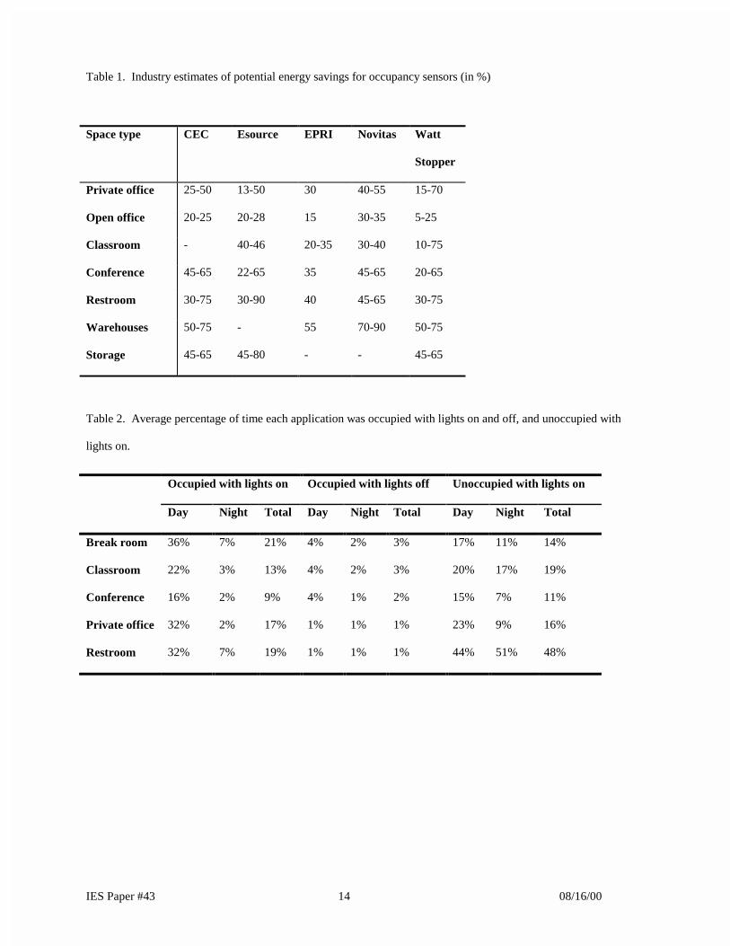
Consequently even within generic space uses categories, industry savings estimates range by a factor of two to three
as shown in Table 1.
These savings estimates have also been criticized as being overly optimistic, given that energy saved during
utility off-peak hours is typically less valuable than energy saved during utility shoulder or peak periods. These
IES Paper #43 3 08/16/00
performance uncertainties make it difficult to predict the economic benefit, and create significant additional
specification risks beyond those borne by demand limiting measures.
Previous Work
Little objective, independent and detailed research information is available on occupancy and lighting
patterns. Single building case studies have also reported a range of savings in a variety of applications. Savings of
10% to 19% have been reported for classrooms (Floyd, et al., 1995; Rundquist, 1996), and of 27% to 43% in private
offices (Jennings et al., 1999; Maniccia et al., 1999; Seattle City Light, 1992). Richman, et al. (1996) reports
potential energy savings of between 45% and 3% for private offices and between 86% and 73% for restrooms.
The primary objective of the present study was to investigate lighting operation and workspace occupancy
patterns across numerous commercial buildings to better quantify the performance estimates of occupancy sensors
across typical space types. By examining how occupants occupy their spaces and manually control their lighting,
and comparing these baselines to modeled occupancy sensor control scenarios, energy and dollars savings potentials
are investigated. Note that the system economics of evaluating energy savings against lamp maintenance costs for
these same control scenarios are evaluated in an associated paper, The Effects of Changes Occupancy Sensor
Timeout Setting on Energy Savings, Lamp Cycling, and Maintenance Costs.
Methodology
Sixty organizations were chosen for study from active participants in the US. Environmental Protection
Agency’s Green Lights Program. The study buildings were located in twenty-four states, and occupied by profit,
not-for profit, service and manufacturing companies, healthcare organizations, primary and secondary education,
and local, state, and federal government entities. The diversity of age, size, efficiency, ownership and occupancy
types for these buildings was intended to represent a typical cross section of the country’s commercial building
stock.
IES Paper #43 4 08/16/00
Rooms for study were identified by on-site facilities management staff as representative of space types
within that building, both in their floorplan, occupancy, and lighting system . All spaces contained manual controls
for the lighting systems, with a minimum connected lighting load of at least 150 watts. A two-week monitoring
period between February and September 1997 was chosen to represent a typical lighting and occupancy schedule.
Data for 180 rooms were originally collected; after eliminating records with inconsistent or incomplete data, the
study database contained 158 rooms categorized by primary occupancy type into 42 restrooms, 37 private offices, 35
classrooms, 33 conference rooms, and 11 break rooms. Rooms were surveyed for occupancy type, dimensions and
lighting system specification. Occupancy and lighting operation data was collected using Wattstopper InteliTimer
Pro£ IT100 data loggers. The logger device recorded the time and state of the light and/or occupancy condition.
Each time occupancy or the lighting condition changed, the logger documented the time of day and the change in
condition. An algorithm was developed to convert the data recorded from the Watt Stopper InteliTimer Pro device
into one-minute increments for the 14-day monitoring period. There were cases when the lights were turned on and
off, but no occupant was detected in the space. This was considered a detection error, and was corrected by
modifying the data set to switch the occupancy condition from unoccupied to occupied for those instances. This
occurred for:
x six of the break rooms with detection errors ranging between one and 181 events (0% to 1% of the
total events)
x 17 of the classrooms with detection errors ranging between one and 2,677 events (0% to 13% of the
total events)
x 16 of the conference rooms with detection errors ranging between one and 1,681 events (0% to 8% of
the total events)
x 17 of the private offices with detection errors ranging between one and 5,686 events (0% to 28% of the
total events)
x seven of the restrooms with detection errors ranging between one and 275 events (0% to 1% of the
total events).
IES Paper #43 5 08/16/00
Descriptive statistics were calculated and cost analyses were performed for weekdays, weekends, and for the
total 14-day monitoring period. Data also were analyzed by separating 24-hour periods into one 12-hour day shift
(Day) and one 12-hour evening shift (Night). Day and night shifts were analyzed from 06:00 to 18:00 and 18:00 to
06:00, respectively. Data presented for weekdays were averaged over the 10 weekdays, and for weekends were
averaged over the four weekend days in the monitoring period. Data presented for the total period were averaged
over the 14-day monitoring period. Baseline occupant switching and occupancy patterns were established using the
collected data on occupancy and light usage. The baseline occupancy and light usage data were then used for
modeling the effects of installing occupancy sensors with 5-, 10-, 15-, and 20-minute time delay periods.
Statistical analyses also were conducted to investigate whether there were significant differences between
the energy use for shift (day or night), time of week (weekday or weekend), and timeout setting, or any interactions
between shift and timeout settings and time of week and timeout settings. These analyses were used to provide
evidence of which differences were real and which occurred by chance. Within-subjects analyses of variance using
repeated measures (ANOVR) were used for the analyes. One analysis compared day and night periods to the
baseline and the four timeout settings. A second analysis compared the weekday and weekend data for a 24-hour
period to the baseline and the four timeout settings. Follow-up tests were conducted using pairwise comparison t-
tests.
For the energy calculations, the total load for each room was used to determine lighting energy use and
waste. Lighting energy use was calculated by multiplying the total lighting load by the time that the lights were on
and the room was occupied. Lighting energy waste was calculated by multiplying the total load by the time that the
lights were on and the room was unoccupied. Total energy savings was determined by applying a flat $0.08/kWh
rate to the modeled energy savings under each control scenario.
IES Paper #43 6 08/16/00
Findings – Baseline data
Total energy savings potential
Determining the basic energy savings potential across applications requires establishing a baseline of observed
occupancy and lighting conditions. Lighting and occupancy use in any space will always fall into one of the
following four conditions:
1. Occupied with the lights on
2. Occupied with the lights off
3. Unoccupied with the lights on
4. Unoccupied with the lights off
Of the four conditions, the first three are of particular interest. Condition one is of interest for garnering
information about how frequently occupants use these types of spaces with the lights on. Conditions two and three
are of interest when considering lighting controls. If occupants frequently occupy a space with the lights off
(condition two), then a manual lighting control device that allows occupants to turn lights off when needed should
be provided. Condition three represents wasted lighting energy by having lights on when spaces are unoccupied.
This condition is of primary importance when considering using automatic occupancy sensor control. Table 2 lists
the average percentage of time each application was in each of the first three occupancy and lighting conditions.
Table 2 illustrates that spaces were infrequently occupied, with the daily percentage of total occupied time
with lights on and off never exceeding 24%. Also, occupants did not diligently turn lights off when they vacated
spaces, with the lighting system in classrooms, conference rooms, and restrooms operating more often when the
occupants were out of the room than in the room. This is intuitively understandable in common area applications
(such as restrooms and conference rooms), where occupants do not feel that the lighting is “theirs” to control. The
split, however, is still fairly even in private offices, indicating that even in personal spaces, occupants were not
diligent about controlling their lighting use. The data shown for condition 2 indicates that occupants rarely occupied
spaces with the lights off, indicating that for these spaces there may be a small potential benefit of installing manual
IES Paper #43 7 08/16/00
controls. Note that since the presence of daylight availability was not documented in this study, however, it is
difficult to compare these results to other studies which have found higher savings potentials from installing manual
controls (Maniccia et al., 1999).
Time of day/week impacts on energy savings
Determining the applicability of occupancy sensors as a control strategy suitable to obtain these savings
requires an examination of when those savings present themselves. As an automatic control strategy, occupancy
sensors work best in areas where occupancy is intermittent and unpredictable. Where the lighting is inadvertently
left on overnight by cleaning, security, or occupants, a more cost effective control strategy may be an education
campaign, or the installation of a simple timeclock. For these reasons, the savings estimates are examined over four
defined periods - weekday days, weekday evenings, weekend days, and weekend evenings.
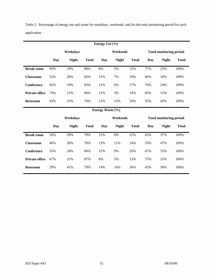
As expected, Table 3 demonstrates that the majority of energy use (76-88%) occurs for all space types
during the weekdays, with 55-85% of total energy use occurring during the day. Likewise, the majority of energy
waste (between 70-87%) occurs during the weekdays, not on the weekends. For all space types except restrooms,
the majority energy waste also occurs during the daytime (53-70%) rather than in the evenings. This indicates that
occupants controlled their lighting poorly during the workday, but were more diligent about turning the lights off
after hours and over weekends. This is particularly true for personal spaces such as private offices, where occupants
feel a high degree of control over their lighting, and less true in common area spaces, such as classrooms and
restrooms, where a high percentages of waste occurred over weekends and after hours. This indicates that time-
based controls (timers, timeclocks) could eliminate a significant amount of energy waste in common areas by
controlling runaway operation after hours and on weekends, however occupancy-based controls would be more
effective given they save not only after hours but also at capturing savings during business hours.
Coincidence of savings with peak demand
Central to defining the economic benefits of occupancy sensors is understanding when the savings
opportunities occur. Most commercial and industrial facilities pay a considerable portion (as high as 40%) of their
IES Paper #43 8 08/16/00
electric energy bill for the peak demand created by the electric loads. Lighting is the second largest contributor to
summer peak demand in commercial facilities, and rivals heating as the largest contributor to a commercial
building’s winter peak. As such, reductions in lighting demand can significantly impact the energy bill.
Occupancy sensors have been criticized in their ability to reduce this peak demand, saving cheaper
kilowatts in the utility’s off-peak billing hours rather than during the peak demand billing period. Although the
value of this savings is highly dependent on how the utility billing rate is structured (time-of-use, annual peak,
ratcheted, etc), it is useful to examine when the potential savings occur to understand how occupancy sensors may
contribute to reducing a building’s peak demand, and reducing demand during peak utility periods. To evaluate this,
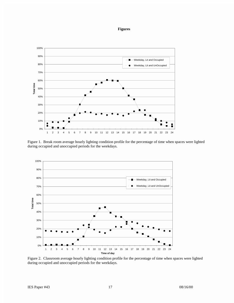
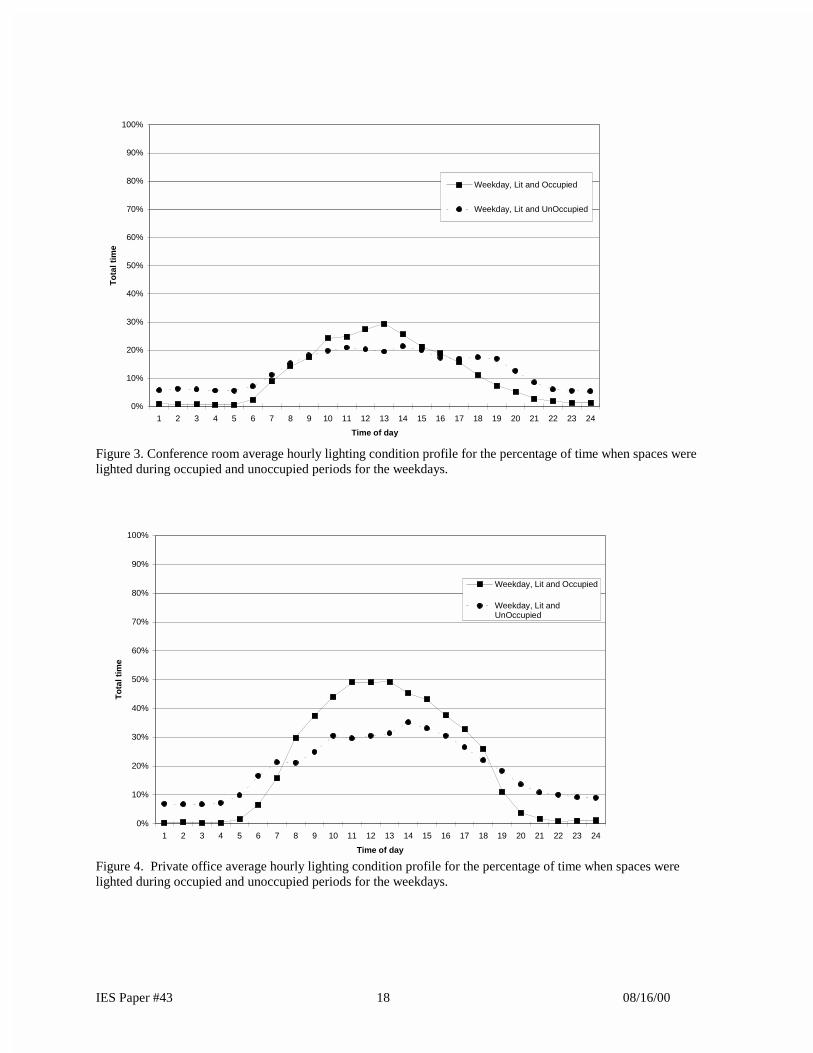
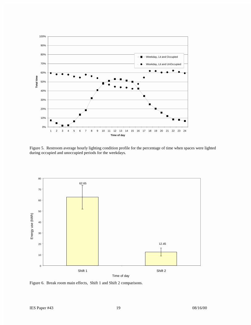
Figures 1-5 illustrate the time of day profiles for when the spaces were lighted and occupied, and lighted and
unoccupied for all weekdays..
Figures 1-5 indicate that the control’s largest contributions to potential savings are not coincident with a
building’s peak occupancy. This is intuitive; when occupancy rises, occupancy-based savings opportunities
diminishes. Although the majority of energy savings from sensors occur during weekdays, the sensors largest
contribution to savings (with the exception of conference rooms and offices) is generally not coincident with a
building’s peak load (10 a.m. to 4 p.m.) or with a utility’s peak billing periods (early afternoon hours). This would
indicate that while sensors can reduce a buildings peak load, they may not be a reliable method of achieving of peak
savings due to the diversity of savings profiles observed among these different space types.
Findings – Occupancy Sensor Simulations
Impact of time-out period on energy savings
Most occupancy sensors are equipped with a variable time delay feature to adjust the time interval between
the last detected motion and the switching off of the lamps. This allows the sensor to be customized to the
application to reduce the chance of lamps switching off when a room is occupied but minor motions are not
detected. Adjusting the time delay creates a tradeoff between saving energy and avoiding occupant complaints.
Longer time delays reduce the incidence of occupant complaints. Shorter time delays increase energy savings
IES Paper #43 9 08/16/00
(particularly in rooms that are infrequently and briefly occupied), but also reduces lamp life from more frequent
lamp cycling. Manufacturers report time delay setting ranging from several seconds to more than 30 minutes.
To examine the impact of time delay on energy savings, control scenarios for 5-, 10-, 15-, and 20-minute
time delays were modeled for each application. Statistical analyses were also conducted to investigate the impact of
time of day, time of week, and timeout setting on energy use. Note that the impact of frequent switching on lamp
and maintenance costs for these same control scenarios are evaluated in an associated paper, The Effects of Changes
Occupancy Sensor Timeout Setting on Energy Savings, Lamp Cycling, and Maintenance Costs.
Statistical Analysis Findings
As discussed in the “Methodology” section, statistical analyses of the energy use data were conducted to
investigate whether there were significant differences between the energy use for Shift (day or night), time of week
(weekday or weekend), and timeout setting, or any interactions between shift and timeout settings and time of week
and timeout settings. The energy use data for each Shift were compared to the baseline and the timeout settings for
one analysis. A second analysis compared the weekday and weekend data for a 24-hour period to the baseline and
the timeout settings.
The statistical analyses addressed the following questions:
x Is there a significant energy use difference between the shifts for the total monitoring period?
x Is there a significant energy use difference between the baseline and each timeout setting?
x Is there a significant energy use difference between weekdays and weekends?
Shift verses timeout settings
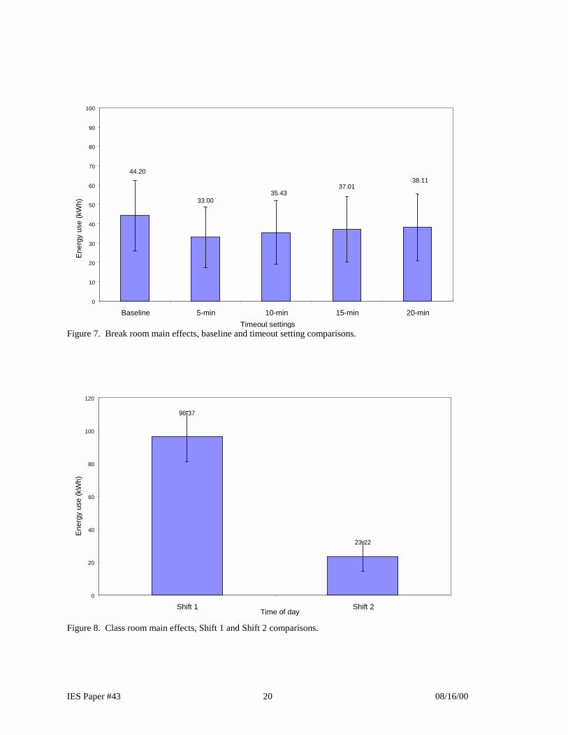
There were no significant interactions between the energy use for each shift and for the timeout settings for
the break rooms or for the classrooms. For both applications, differences between the main effects (Shifts 1 and 2)
were significant (p < 0.01 for the break rooms, and p < 0.001 for the classrooms). Differences between the timeout
setting main effects were also significant for both of these applications (p < 0.01 for the break rooms, and p < 0.01
IES Paper #43 10 08/16/00
for the classrooms). Figures 6 through 9 illustrate the results of the main effects tests for the break rooms and
classrooms, respectively.
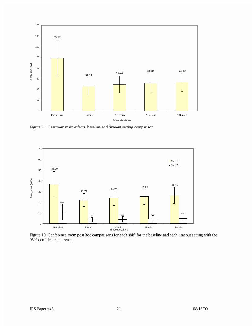
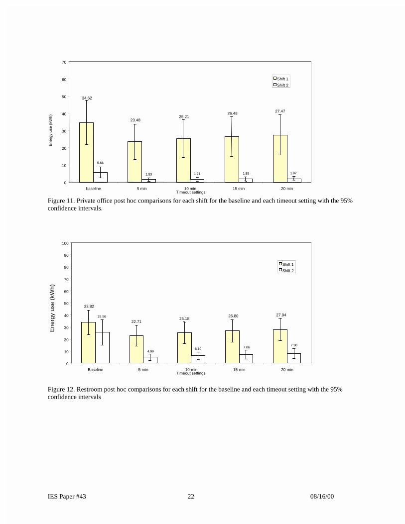
Significant interactions occurred between energy use for each shift and timeout settings for the conference
rooms (p < 0.05), private offices (p < 0.001), and restrooms (p < 0.01). Follow-up tests illustrated that differences
between the shifts at each timeout setting and the baseline condition were all significant (p < 0.001) for all three
applications. Differences between the baseline condition and each timeout setting were all significant for Shift 1 for
all three applications (p < 0.001). Differences between the baseline condition and each timeout setting also were
significant for Shift 2 for all three applications (the conference rooms and private offices [p < 0.01] and restrooms
[p <0.001]). Figures 10 through 12 illustrate the results of the follow-up tests with the 95% confidence intervals.
Figures 6 through 12 illustrate that more energy is used during the day than at night, which would be
expected of these types of applications. They also show that installing occupancy sensors decreases baseline energy
use, and that energy use increases as the timeout setting increases because lights remain on for longer periods of
time.
Time of week verses timeout settings
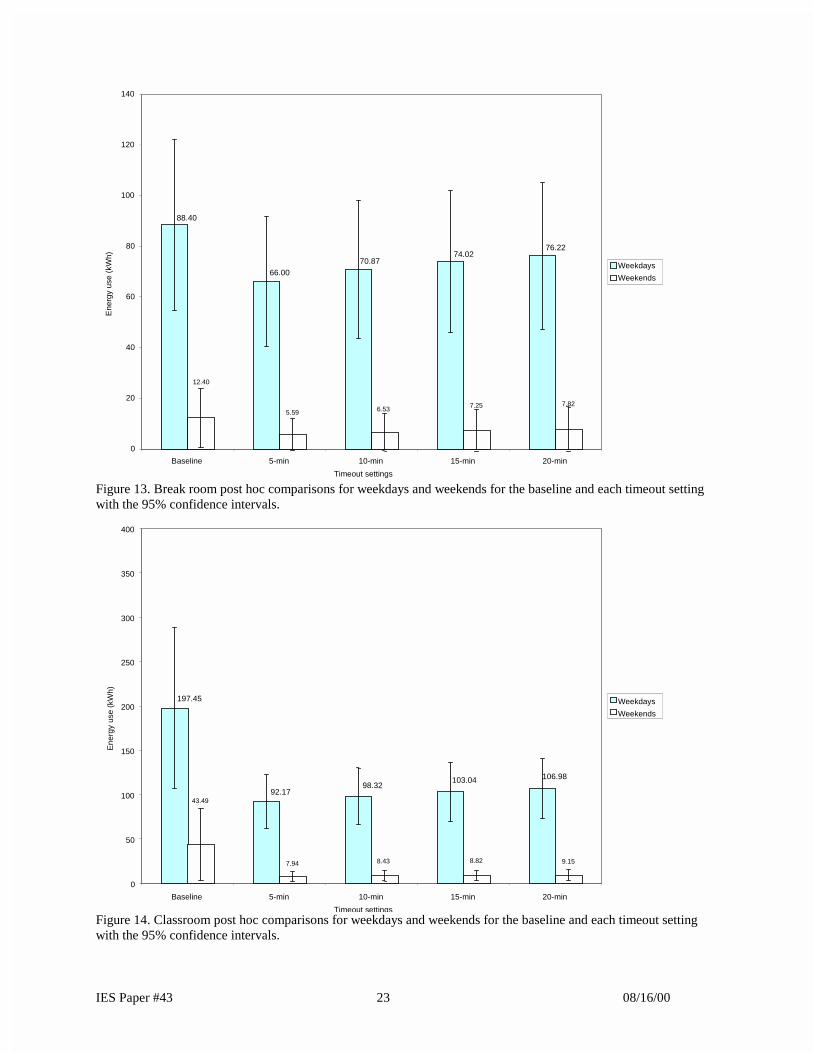
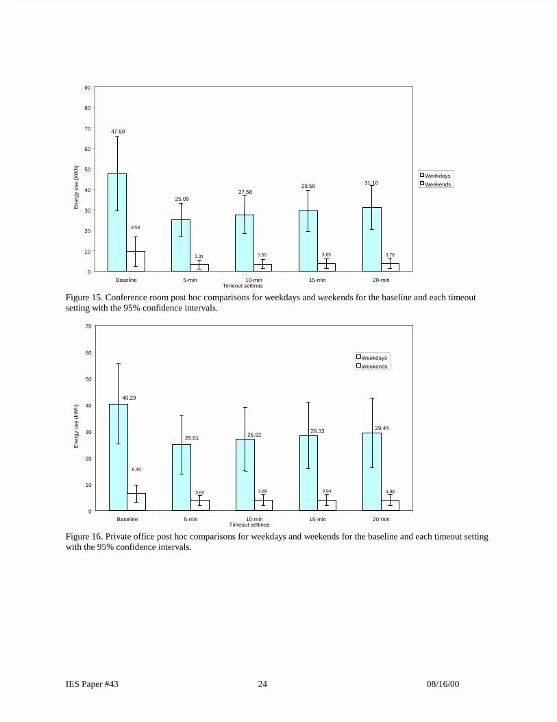
There were significant interactions between the energy use for time of week and timeout settings for all five
applications (p < 0.05 for the break rooms and p < 0.001 for the classrooms, conference rooms, private offices, and
restrooms). Follow-up tests illustrated that differences between the energy use values for the weekdays and
weekends at each timeout setting and the baseline were significant for all of the applications (p < 0.01 for the break
rooms, and p < 0.001 for the classrooms, conference rooms, private offices, and restrooms). Differences between the
energy use values for the baseline and each timeout setting for the weekdays also were significant for each
application (p < 0.01 for the break rooms and classrooms, and p < 0.001 for the conference rooms, private offices,
and restrooms). Differences between the energy use values for the baseline and each timeout setting for the
weekends were not significant for the break rooms, classrooms, and conference rooms. However, these differences
were significant for the private offices (p < 0.05) and restrooms (p < 0.001). These results are illustrated in Figures
13 through 17.
IES Paper #43 11 08/16/00
The two main points that can be taken away from this analysis are:
x the differences between the energy use for each timeout setting and the baseline for each application were
all significant for each shift. This indicates that energy savings can be achieved during the day and at night
using occupancy sensors.
x the differences between the energy use for each timeout setting and the baseline for each application were
all significant for the weekdays, but varied by application for the weekends. This indicates that energy
savings can be achieved during the week for all applications, and during the weekend for private offices
and restrooms.
Effects of Time Delay on Energy and Cost Savings
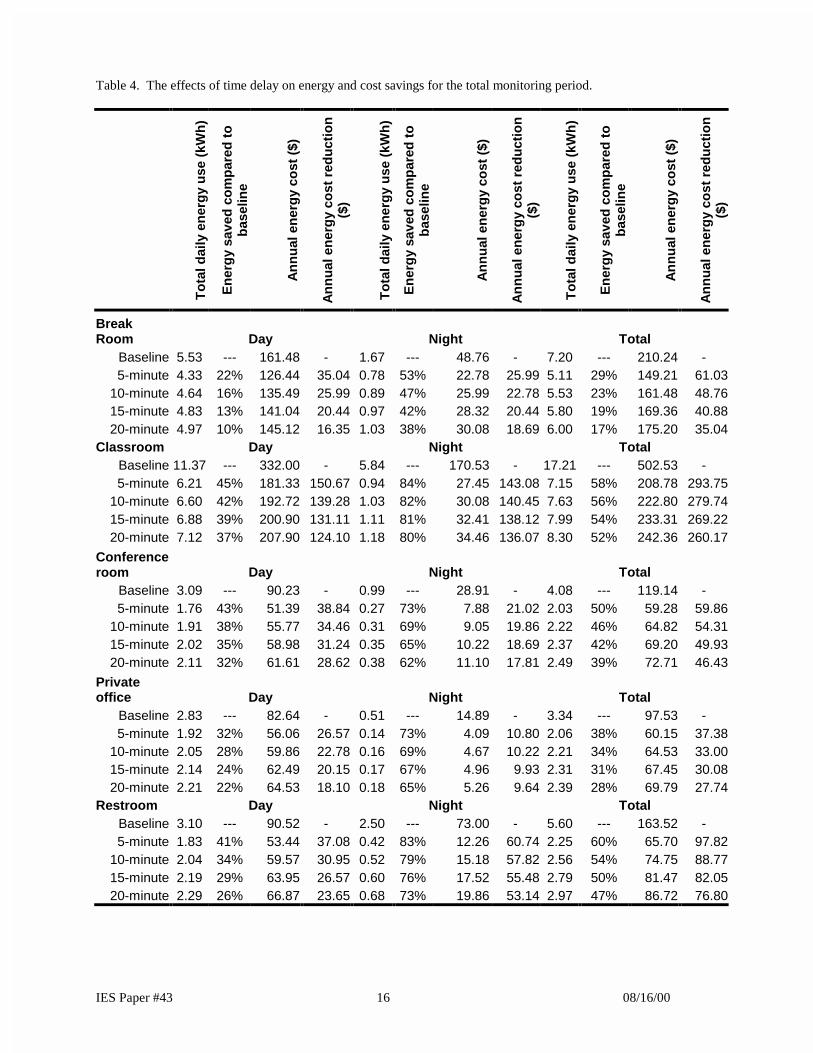
As demonstrated in Table 4, the savings estimates were considerable across all space types (ranging from
17-60%), and consistent with the ranges of industry estimates provided in Table 1. Table 4 illustrates that both
application and time delay selection significantly impacts the quantity of available savings. For this data set,
restrooms showed the highest overall savings, followed by classrooms, conference rooms, and private offices. Break
rooms showed the lowest overall savings. The range of savings between the shortest and longest time out setting
varied with application as well because of the occupancy pattern differences among the applications. Classrooms
had the smallest savings difference between the 5- and 20-minute time out settings (6%) and restrooms had the
largest difference (13%).
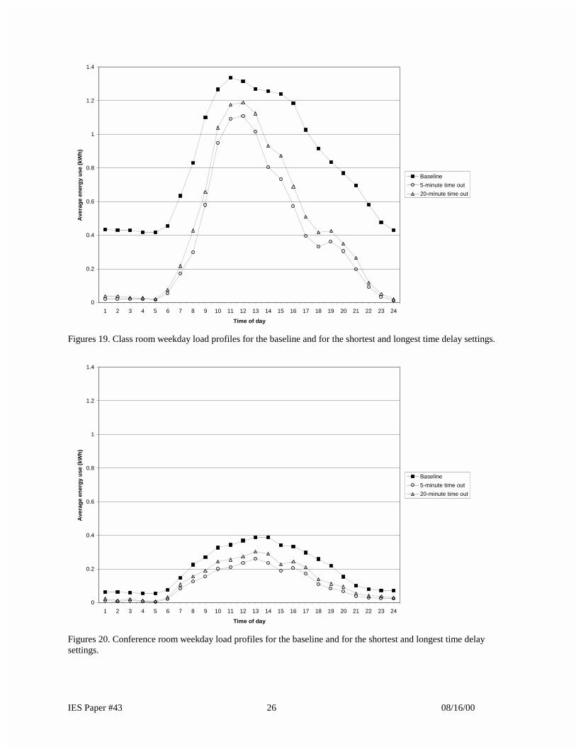
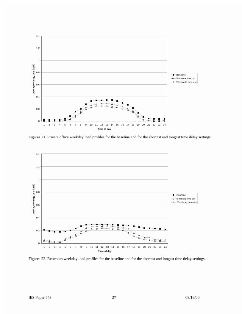
Figures 18-22 illustrate the load profiles for the baseline energy use and modeled energy use under 5 and
20 minute simulated delay conditions. These figures graphically depict the differences found in the energy savings
captured between the longest and shortest time delays. These figures also confirm the observations found from the
baseline occupancy and lighting conditions depicted in Figures 1-5; although the majority of energy savings from
sensors occur during weekdays, the sensors largest contribution to savings (with the exception of conference rooms
and offices) is generally not coincident with a building’s peak load or with a utility’s peak billing periods. This
suggests that while sensors can reduce a buildings peak load, sensors may not be a reliable method of achieving
peak savings in buildings with a diversity of space types.
IES Paper #43 12 08/16/00
Conclusions/Recommendations for Future Work
People do not occupy spaces for a large percentage of time, and are not diligent about controlling the
lighting in their spaces both during the workday, and after hours and weekends. This applies to both public spaces as
well as personal spaces. The majority of this energy waste occurs during the weekdays, not during the weeknights
or over the weekends. This pattern of energy waste is particularly suited to control by occupancy sensors, which not
only prevent runaway operation after typical business hours, but also capture savings during the business day.
Although the majority of observed savings opportunities occurred during the weekday, the peak savings
contributions from occupancy sensors for several space types did not fall within the typical peak utility billing
periods (early afternoon) or peak commercial building demand periods (10 a.m. to 4 p.m.). This suggests that while
sensors may help to save expensive kilowatt-hours, they would have a variable effect at reducing a building’s peak
demand, given their variable performance in when they provide high levels of savings among the various space
types. This would be a useful topic of additional research, where assigning specific kilowatt-hour rates to each
kilowatt-hour saved would yield more accurate indication of the economic benefits of installing sensors within these
various space types.
Finally, modeling control scenarios with 5- to 20-minute time delay periods indicated savings potentials
that were within the ranges suggested by the industry estimates. The time delay settings used for these analyses
showed that energy savings can range from between 6% and 13% depending on the application and on which time
out setting is used. In addition, the highest savings were obtained in the restroom application (47% to 60%), and the
lowest in the break rooms (17% to 29%). Thus, the time delay selection can greatly impact energy savings.
Although these savings are significant they do not consider the increased maintenance lamp and labor replacement
costs that could result due to more frequent lamp switching. This is evaluated in a related paper entitled The Effects
of Changes Occupancy Sensor Timeout Setting on Energy Savings, Lamp Cycling, and Maintenance Costs.
IES Paper #43 13 08/16/00
References
Audin, L., 1999. Occupancy Sensors: Promises and Pitfalls. Esource Tech Update, TU-93-8, Boulder CO.. California Energy Commission (CEC), 1992. Occupant Sensors. Advanced Lighting Guidelines, P400-93-014.
California Energy Commission, Sacramento, CA. Electric Power Research Institute (EPRI), 1992. Occupancy Sensors: Positive On/Off Lighting Control, BR-100323.
Electric Power Research Institute, Palo Alto, CA. Floyd, David B., Danny S. Parker, Janet E. R. McIlvaine, and John R. Sherwin. 1995. Energy efficiency technology
demonstration project for Florida educational facilities: Occupancy sensors, FSEC-CR-867-95. Cocoa FL: Florida Solar Energy Center, Building Design Assistance Center. Accessed February 23, 2000 at http//:www.fsec.ucf.edu/~bdac/pubs/CR867/Cr-867.htm.
Maniccia, Dorene, Burr Rutledge, Mark S. Rea, and Wayne Morrow. 1999. Occupant use of manual lighting controls in private offices. Journal of the Illuminating Engineering Society 28(2):42-56.
R.A. Rundquist Associates. 1996. Lighting controls: Patterns for design, TR-107230. Palo Alto, CA: Electric Power Research Institute.
Richman, E. E., A. L. Dittmer, and J. M. Keller. 1996. Field analysis of occupancy sensor operation: Parameters affecting lighting energy savings. Journal of the Illuminating Engineering Society 25(1):83-92.
Seattle City Light. Energy Management Services Division. 1992. Case study on occupant sensors as an office lighting control strategy. Seattle WA: Seattle City Light
Jennings, Judith D., Francis M. Rubinstein, Dennis DiBartolomeo, Steven L. Blanc. 1999. Comparison of control options in private offices in an advanced lighting controls testbed. Proceedings of the Illuminating Engineering Society, Paper #44. 275 – 298.
The Watt Stopper. [1998] Applications & savings. Automatic Lighting, HVAC, and Office Power Controls. Santa Clara, CA: The Watt Stopper
IES Paper #43 14 08/16/00
Table 1. Industry estimates of potential energy savings for occupancy sensors (in %)
Space type CEC Esource EPRI Novitas Watt
Stopper
Private office 25-50 13-50 30 40-55 15-70
Open office 20-25 20-28 15 30-35 5-25
Classroom - 40-46 20-35 30-40 10-75
Conference 45-65 22-65 35 45-65 20-65
Restroom 30-75 30-90 40 45-65 30-75
Warehouses 50-75 - 55 70-90 50-75
Storage 45-65 45-80 - - 45-65
Table 2. Average percentage of time each application was occupied with lights on and off, and unoccupied with
lights on.
Occupied with lights on Occupied with lights off Unoccupied with lights on
Day Night Total Day Night Total Day Night Total
Break room 36% 7% 21% 4% 2% 3% 17% 11% 14%
Classroom 22% 3% 13% 4% 2% 3% 20% 17% 19%
Conference 16% 2% 9% 4% 1% 2% 15% 7% 11%
Private office 32% 2% 17% 1% 1% 1% 23% 9% 16%
Restroom 32% 7% 19% 1% 1% 1% 44% 51% 48%
IES Paper #43 15 08/16/00
Table 3. Percentage of energy use and waste for weekdays, weekends, and for the total monitoring period for each
application.
Energy Use (%)
Weekdays Weekends Total monitoring period
Day Night Total Day Night Total Day Night Total
Break room 69% 19% 88% 8% 5% 12% 77% 23% 100%
Classroom 55% 26% 82% 11% 7% 18% 66% 34% 100%
Conference 65% 19% 83% 11% 6% 17% 76% 24% 100%
Private office 74% 12% 86% 11% 3% 14% 85% 15% 100%
Restroom 43% 33% 76% 12% 12% 24% 55% 45% 100%
Energy Waste (%)
Weekdays Weekends Total monitoring period
Day Night Total Day Night Total Day Night Total
Break room 50% 29% 79% 12% 8% 21% 63% 37% 100%
Classroom 40% 36% 76% 13% 11% 24% 53% 47% 100%
Conference 55% 24% 80% 12% 9% 20% 67% 33% 100%
Private office 67% 21% 87% 8% 5% 13% 75% 25% 100%
Restroom 29% 41% 70% 14% 16% 30% 42% 58% 100%
IES Paper #43 16 08/16/00
Table 4. The effects of time delay on energy and cost savings for the total monitoring period.
To
tal d
aily
en
erg
y u
se (
kWh
)
En
erg
y sa
ved
co
mp
ared
to
b
asel
ine
An
nu
al e
ner
gy
cost
($)
An
nu
al e
ner
gy
cost
red
uct
ion
($
)
To
tal d
aily
en
erg
y u
se (
kWh
)
En
erg
y sa
ved
co
mp
ared
to
b
asel
ine
An
nu
al e
ner
gy
cost
($)
An
nu
al e
ner
gy
cost
red
uct
ion
($
)
To
tal d
aily
en
erg
y u
se (
kWh
)
En
erg
y sa
ved
co
mp
ared
to
b
asel
ine
An
nu
al e
ner
gy
cost
($)
An
nu
al e
ner
gy
cost
red
uct
ion
($
)
Break Room Day Night Total
Baseline 5.53 --- 161.48 - 1.67 --- 48.76 - 7.20 --- 210.24 - 5-minute 4.33 22% 126.44 35.04 0.78 53% 22.78 25.99 5.11 29% 149.21 61.03
10-minute 4.64 16% 135.49 25.99 0.89 47% 25.99 22.78 5.53 23% 161.48 48.76 15-minute 4.83 13% 141.04 20.44 0.97 42% 28.32 20.44 5.80 19% 169.36 40.88 20-minute 4.97 10% 145.12 16.35 1.03 38% 30.08 18.69 6.00 17% 175.20 35.04
Classroom Day Night Total Baseline 11.37 --- 332.00 - 5.84 --- 170.53 - 17.21 --- 502.53 - 5-minute 6.21 45% 181.33 150.67 0.94 84% 27.45 143.08 7.15 58% 208.78 293.75
10-minute 6.60 42% 192.72 139.28 1.03 82% 30.08 140.45 7.63 56% 222.80 279.74 15-minute 6.88 39% 200.90 131.11 1.11 81% 32.41 138.12 7.99 54% 233.31 269.22 20-minute 7.12 37% 207.90 124.10 1.18 80% 34.46 136.07 8.30 52% 242.36 260.17
Conference room Day Night Total
Baseline 3.09 --- 90.23 - 0.99 --- 28.91 - 4.08 --- 119.14 - 5-minute 1.76 43% 51.39 38.84 0.27 73% 7.88 21.02 2.03 50% 59.28 59.86
10-minute 1.91 38% 55.77 34.46 0.31 69% 9.05 19.86 2.22 46% 64.82 54.31 15-minute 2.02 35% 58.98 31.24 0.35 65% 10.22 18.69 2.37 42% 69.20 49.93 20-minute 2.11 32% 61.61 28.62 0.38 62% 11.10 17.81 2.49 39% 72.71 46.43
Private office Day Night Total
Baseline 2.83 --- 82.64 - 0.51 --- 14.89 - 3.34 --- 97.53 - 5-minute 1.92 32% 56.06 26.57 0.14 73% 4.09 10.80 2.06 38% 60.15 37.38
10-minute 2.05 28% 59.86 22.78 0.16 69% 4.67 10.22 2.21 34% 64.53 33.00 15-minute 2.14 24% 62.49 20.15 0.17 67% 4.96 9.93 2.31 31% 67.45 30.08 20-minute 2.21 22% 64.53 18.10 0.18 65% 5.26 9.64 2.39 28% 69.79 27.74
Restroom Day Night Total Baseline 3.10 --- 90.52 - 2.50 --- 73.00 - 5.60 --- 163.52 - 5-minute 1.83 41% 53.44 37.08 0.42 83% 12.26 60.74 2.25 60% 65.70 97.82
10-minute 2.04 34% 59.57 30.95 0.52 79% 15.18 57.82 2.56 54% 74.75 88.77 15-minute 2.19 29% 63.95 26.57 0.60 76% 17.52 55.48 2.79 50% 81.47 82.05 20-minute 2.29 26% 66.87 23.65 0.68 73% 19.86 53.14 2.97 47% 86.72 76.80
IES Paper #43 17 08/16/00
Figures
Figure 1. Break room average hourly lighting condition profile for the percentage of time when spaces were lighted during occupied and unoccupied periods for the weekdays.
Figure 2. Classroom average hourly lighting condition profile for the percentage of time when spaces were lighted during occupied and unoccupied periods for the weekdays.
0%
10%
20%
30%
40%
50%
60%
70%
80%
90%
100%
1 2 3 4 5 6 7 8 9 10 11 12 13 14 15 16 17 18 19 20 21 22 23 24
To
tal t
ime
Weekday, Lit and Occupied
Weekday, Lit and UnOccupied
0%
10%
20%
30%
40%
50%
60%
70%
80%
90%
100%
1 2 3 4 5 6 7 8 9 10 11 12 13 14 15 16 17 18 19 20 21 22 23 24
Time of day
To
tal t
ime
Weekday, Lit and Occupied
Weekday, Lit and UnOccupied
IES Paper #43 18 08/16/00
Figure 3. Conference room average hourly lighting condition profile for the percentage of time when spaces were lighted during occupied and unoccupied periods for the weekdays.
Figure 4. Private office average hourly lighting condition profile for the percentage of time when spaces were lighted during occupied and unoccupied periods for the weekdays.
0%
10%
20%
30%
40%
50%
60%
70%
80%
90%
100%
1 2 3 4 5 6 7 8 9 10 11 12 13 14 15 16 17 18 19 20 21 22 23 24
Time of day
To
tal t
ime
Weekday, Lit and Occupied
Weekday, Lit and UnOccupied
0%
10%
20%
30%
40%
50%
60%
70%
80%
90%
100%
1 2 3 4 5 6 7 8 9 10 11 12 13 14 15 16 17 18 19 20 21 22 23 24
Time of day
To
tal t
ime
Weekday, Lit and Occupied
Weekday, Lit andUnOccupied
IES Paper #43 19 08/16/00
Figure 5. Restroom average hourly lighting condition profile for the percentage of time when spaces were lighted during occupied and unoccupied periods for the weekdays.
62.65
12.45
0
10
20
30
40
50
60
70
80
Shift 1 Shift 2
Ene
rgy
use
(kW
h)
Time of day
Figure 6. Break room main effects, Shift 1 and Shift 2 comparisons.
0%
10%
20%
30%
40%
50%
60%
70%
80%
90%
100%
1 2 3 4 5 6 7 8 9 10 11 12 13 14 15 16 17 18 19 20 21 22 23 24
Time of day
To
tal t
ime
Weekday, Lit and Occupied
Weekday, Lit and UnOccupied
IES Paper #43 20 08/16/00
38.1137.01
35.4333.00
44.20
0
10
20
30
40
50
60
70
80
90
100
Baseline 5-min 10-min 15-min 20-min
Ene
rgy
use
(kW
h)
Timeout settings Figure 7. Break room main effects, baseline and timeout setting comparisons.
23.22
96.37
0
20
40
60
80
100
120
Shift 1 Shift 2
Ene
rgy
use
(kW
h)
Time of day
Figure 8. Class room main effects, Shift 1 and Shift 2 comparisons.
IES Paper #43 21 08/16/00
98.72
46.08 49.16 51.52 53.49
0
20
40
60
80
100
120
140
160
Baseline 5-min 10-min 15-min 20-min
Ene
rgy
use
(kW
h)
Timeout settings
Figure 9. Classroom main effects, baseline and timeout setting comparison
26.4125.21
23.7321.78
36.90
4.694.293.853.31
10.69
0
10
20
30
40
50
60
70
Baseline 5-min 10-min 15-min 20-min
Ene
rgy
use
(kW
h)
Shift 1
Shift 2
Timeout settings Figure 10. Conference room post hoc comparisons for each shift for the baseline and each timeout setting with the 95% confidence intervals.
IES Paper #43 22 08/16/00
27.4726.4825.21
23.48
34.62
1.971.851.711.53
5.66
0
10
20
30
40
50
60
70
baseline 5 min 10 min 15 min 20 min
Shift 1
Shift 2
Timeout settings
Ene
rgy
use
(kW
h)
Figure 11. Private office post hoc comparisons for each shift for the baseline and each timeout setting with the 95% confidence intervals.
27.9426.8025.18
22.71
33.82
7.907.066.10
4.99
25.56
0
10
20
30
40
50
60
70
80
90
100
Baseline 5-min 10-min 15-min 20-min
Shift 1
Shift 2
Timeout settings
Ene
rgy
use
(kW
h)
Figure 12. Restroom post hoc comparisons for each shift for the baseline and each timeout setting with the 95% confidence intervals
IES Paper #43 23 08/16/00
76.22 74.02
70.87 66.00
88.40
7.82 7.25 6.53 5.59
12.40
0
20
40
60
80
100
120
140
Baseline 5-min 10-min 15-min 20-min
Ene
rgy
use
(kW
h)
Weekdays Weekends
Timeout settings Figure 13. Break room post hoc comparisons for weekdays and weekends for the baseline and each timeout setting with the 95% confidence intervals.
106.98103.0498.32
92.17
197.45
9.158.828.437.94
43.49
0
50
100
150
200
250
300
350
400
Baseline 5-min 10-min 15-min 20-min
Weekdays
Weekends
Timeout settings
Ene
rgy
use
(kW
h)
Figure 14. Classroom post hoc comparisons for weekdays and weekends for the baseline and each timeout setting with the 95% confidence intervals.
IES Paper #43 24 08/16/00
31.1029.50
27.5825.09
47.59
3.793.653.503.31
9.58
0
10
20
30
40
50
60
70
80
90
Baseline 5-min 10-min 15-min 20-min
Weekdays
Weekends
Timeout settings
Ene
rgy
use
(kW
h)
Figure 15. Conference room post hoc comparisons for weekdays and weekends for the baseline and each timeout setting with the 95% confidence intervals.
29.4428.3326.92
25.01
40.29
3.983.943.893.82
6.40
0
10
20
30
40
50
60
70
Baseline 5-min 10-min 15-min 20-min
Weekdays
Weekends
Timeout settings
Ene
rgy
use
(kW
h)
Figure 16. Private office post hoc comparisons for weekdays and weekends for the baseline and each timeout setting with the 95% confidence intervals.
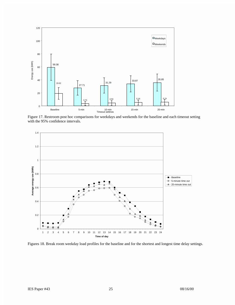
IES Paper #43 25 08/16/00
35.8533.8731.29
27.71
59.38
5.745.164.503.73
19.02
0
20
40
60
80
100
120
Baseline 5-min 10-min 15-min 20-min
Weekdays
Weekends
Timeout settings
Ene
rgy
use
(kW
h)
Figure 17. Restroom post hoc comparisons for weekdays and weekends for the baseline and each timeout setting with the 95% confidence intervals.
0
0.2
0.4
0.6
0.8
1
1.2
1.4
1 2 3 4 5 6 7 8 9 10 11 12 13 14 15 16 17 18 19 20 21 22 23 24
Time of day
Ave
rag
e en
erg
y u
se (k
Wh
)
Baseline
5-minute time out
20-minute time out
Figures 18. Break room weekday load profiles for the baseline and for the shortest and longest time delay settings.
IES Paper #43 26 08/16/00
0
0.2
0.4
0.6
0.8
1
1.2
1.4
1 2 3 4 5 6 7 8 9 10 11 12 13 14 15 16 17 18 19 20 21 22 23 24
Time of day
Ave
rag
e en
erg
y u
se (k
Wh
)
Baseline
5-minute time out
20-minute time out
Figures 19. Class room weekday load profiles for the baseline and for the shortest and longest time delay settings.
0
0.2
0.4
0.6
0.8
1
1.2
1.4
1 2 3 4 5 6 7 8 9 10 11 12 13 14 15 16 17 18 19 20 21 22 23 24
Time of day
Ave
rag
e en
erg
y u
se (k
Wh
)
Baseline
5-minute time out
20-minute time out
Figures 20. Conference room weekday load profiles for the baseline and for the shortest and longest time delay settings.
IES Paper #43 27 08/16/00
0
0.2
0.4
0.6
0.8
1
1.2
1.4
1 2 3 4 5 6 7 8 9 10 11 12 13 14 15 16 17 18 19 20 21 22 23 24
Time of day
Ave
rag
e en
erg
y u
se (k
Wh
)
Baseline
5-minute time out
20-minute time out
Figures 21. Private office weekday load profiles for the baseline and for the shortest and longest time delay settings.
0
0.2
0.4
0.6
0.8
1
1.2
1.4
1 2 3 4 5 6 7 8 9 10 11 12 13 14 15 16 17 18 19 20 21 22 23 24
Time of day
Ave
rag
e en
erg
y u
se (k
Wh
)
Baseline
5-minute time out
20-minute time out
Figures 22. Restroom weekday load profiles for the baseline and for the shortest and longest time delay settings.