an analysis of major determinants of poverty in...
TRANSCRIPT

An Analysis of Major Determinants of Poverty in Agriculture Sector in
Pakistan
Dawood Jan, Anwar Chishti, and Phillip Eberle*
Department of Agricultural Economics
NWFP Agricultural University
Peshawar
Pakistan
*Department of Agribusiness Economics
Southern Illinois University Carbondale
Carbondale, IL 62901
Selected Paper prepared for presentation at the American Agricultural Economics
Association Annual Meeting, Orlando, FL, July 27-29, 2008.
Copyright 2008 by Dawood Jan, Anwar Chishti, and Phillip Eberle. All rights reserved. Readers may
make verbatim copies of this document for non-commercial purposes by any means, provided that this
copyright notice appears on all such copies.
1
An Analysis of Major Determinants of Poverty in Agriculture Sector in Pakistan
Abstract
This study is an attempt to highlight the need to prioritize the agriculture sector in policies aimed
at alleviating poverty. The objectives are (1) to estimate and compare the incidence of poverty
across various sectors of the economy with special focus on the agricultural sector and (2) to
identify the major determinants of poverty in the agriculture sector. Poverty is measured in
terms of head count, poverty gap and severity of poverty indices all determined as a function of
household consumption level. Households with adult equivalent consumption below a
consumption level necessary to acquire basic needs are defined as poor. The estimated
measures of poverty are used to compare incidence of poverty across sectors of the economy.
Adult equivalent consumption is then regressed against a series of explanatory variables to
identify determinants of poverty. Results from consumption model are then simulated to gauge
impact of various policy scenarios on poverty levels. Data sets are from the 2001 Pakistan
Integrated Household Survey and 2005 Living Standard Measurement Survey.

2
An analysis of Major Determinants of Poverty in Agriculture Sector in
Pakistan
Introduction
In Pakistan around two-third of the population live in rural areas and agriculture is a major
source of livelihood to a majority of them. It contributes nearly 23 percent to the Pakistan‟s
Gross Domestic Product (GDP) while employing 42 percent of the labor force (GoP 2004-05,
p.9). This simple fact suggest that agriculture contributes less to the national GDP relative to its
size of population and labor force compared to other sectors of the economy. So on any living
standard scale, people associated with agriculture fare low compared to other sectors.
This simple fact is further supported by a review of literature indicating that in developing
countries: (a) There exist a strong positive correlation between share of agriculture GDP and
incidence of poverty suggesting that majority of poor reside in agriculture sector. (b) Countries
with higher agriculture employment experience increased level of poverty. (c) Agriculture
accommodates most of the unpaid family members wherein incidence of poverty is higher as
compared to properly and regularly paid employees (FAO 2005, p.61-62).
The role of agriculture sector in poverty alleviation has also been emphasized by many studies.
For instance, Pasha and Palanivel (2004) analyzed pro-poor growth and policies in Asian
countries and concluded that “the key determinants of the degree of pro-poor growth are the rates
of agricultural growth and employment generation”. A study by FAO (2004a), covering 11
countries, examined the effect of agriculture-led growth on poverty and found that “the pro-poor
role of agriculture can be dramatic and much more effective in reducing poverty and hunger than
other sectors in both urban and rural areas”. Examining the link between agriculture growth and

3
rural poverty, Malik (2005, p.1) stated that relationship between poverty reduction and overall
economic growth is not as clear as the one between poverty reduction and agriculture growth.
Along with the poverty growth nexus, the incidence of poverty is also viewed in the context of
various individual level characteristics of the household. Here poverty of a household is studied
as a function of the extent and level of various human and physical endowments of a household.
There is an abundance of recent literature that links poverty to various characteristics of a
household such as those related to demography, education, physical assets, community and
infrastructure. While most of the studies present this link in the form of bivariate analysis in a
shape of poverty profiles, recent emphasis is more on multivariate analysis that captures the
effect of one variable conditional on the impact of other variables. Some recent examples of such
studies include Fagernas and Wallace (2007), Datt and Jolliffe (2005), Simler et al. (2004) to
quote a few.
This study is a mix of both. In the first place we tried to estimate and capture change in the
incidence of poverty over time given the growth in overall and agricultural economy with a focus
on the agriculture sector. Secondly we went on to identify the major determinants of poverty in
the agriculture sector.
Background
Poverty is an international phenomenon. Some recent global estimates (based on one dollar a
day) suggest around 1.2 billion people live in poverty and more than 850 million does not have
enough access to sufficient food for an active and healthy life (FAO 2005, Forward). Of the total
global population who live on less than a dollar a day, 1.089 billion live in developing countries
and 0.431 billion live in South Asia, the region to which Pakistan is a part of; while of the total

4
undernourished people, 815 million and 301 million people reside in developing countries and
South Asian Countries respectively (FAO 2005, p.80).
As far as Pakistan is concerned, it ranked 136 based on Human Development Index out of a total
of 177 countries; well behind some of its neighboring countries like Sri Lanka with a ranking of
99, India 128 and Bhutan 133. Recent estimates of people living in poverty, based on 1 dollar a
day, suggest that 17 % of the population live below poverty line in 2005 whereas based on 2
dollar a day criteria, the figure stand out at 73.6 %, more than two third of the population (HDR
2007-08, p. 231 & 239).
FAO estimates for 2001-02 pointed out that 20% of Pakistan‟s population is undernourished and
32.6% of its population is under poverty line (FAO 2005, p.150 & 177). Cheema (2005, p.15 &
16) estimated poverty, using Household Income and Expenditure Survey (HIES) 2001-02, at
34.46%, including 39.26% in rural areas and 22.69% in urban areas. While based on the recent
available Living Standard Measurement Survey (LSMS), the government of Pakistan claimed
that over all poverty has declined from 34.46% in 2001-02 to 23.9% in 2004-05, showing a
decline from 39.26 to 28.13% in rural areas and from 22.69% to 14.94% in urban areas (GoP
2006, p.55 & UNDP 2007, p.9). This substantial decline in poverty is inherent in the
methodology that is followed by the government of Pakistan for the recent estimates. On the one
hand it did correctly, by keeping the base poverty line fixed and updating it by the inflation rate
that has occurred between the two periods i.e. 2001-02 and 2004-05 and by paying heed to one
of the main criticism that Pakistan‟s poverty lines are not consistent and hence not comparable
(Kakwani 2003, p.10). But the real issue is the way the base poverty line is updated. In Pakistan
poverty line is updated using the Consumer Price Index (CPI). Though, the use of CPI for
calculating the inflation rate and subsequently for updating poverty line is a standard practice in

5
many countries. Its use in case of Pakistan is questionable as its coverage is only limited to the
urban areas whereas a vast majority, around two-third, live in rural areas. So the use of CPI for
updating the poverty line for 2004-05 seems to have under-estimated the incidence of poverty
line (World Bank 2006, p.4). Updating the poverty line using CPI affects not only the incidence
of poverty at the national level but also its decomposition across regions (urban/rural) and sectors
of the economy including the agriculture sector.
In this backdrop we attempted to first calculate the poverty line using HIES 2001-02 that serve as
base poverty line and then updated it for LSMS 2004-05 by a survey based inflation rate
(commonly known as the Tranqvist Price Index (TPI)). This TPI method helped in creating an
overall picture depicting the change in overall incidence of poverty at the national, regional and
sectoral level. An attempt has also been made to show „who‟ benefited from the overall growth
that occurred between the two survey periods before modeling the determinants of poverty,
taking into account the individual and community level characteristics of the households related
to agriculture. The following step explains the estimation of poverty line for the base survey
year, its subsequent inflation by the TPI for the second survey year and the estimation results for
both survey years.
Absolute Poverty in Pakistan: Data and Method
The study used the Pakistan Integrated Household Survey (PIHS/HIES) data set of 2001-02 and
HIES part of Pakistan Social and Living Standard Measurement Survey (PSLM) 2004-05. These
surveys have representative samples from all four federating units of Pakistan i.e. Punjab, Sind,
NWFP and Baluchistan on urban-rural basis and provide detailed information on food and non-
food consumption items of households. Only those households were included in the analyses that

6
have reported food consumption expenditure along with other non-food consumption
expenditure. Table 1 shows the overall sample size, with province wise urban/rural breakdown.
Both the PIHS 2001-02 and LSMS 2004-05 provide a comprehensive coverage of consumption
aggregates. This consumption aggregate includes both actual and imputed expenditure and
include not only actual purchases but also self produced and consumed items, consumption of
items that have been received as gift or assistance and those that have been given as wage or
salary in kind. Consumption aggregate is a comprehensive one as it consists of almost all food
items, fuel and utilities, housing (rent, imputed rent and minor repairs), frequent nonfood
expenses (household laundry and cleaning, personal care products and services etc.) and other
nonfood expenses (clothes, footwear, schooling, stationary, transportation, health related
expenses etc.). However, expenses such as taxes, fines, and expenses on marriage/funeral have
been excluded from the consumption aggregate.
Choosing an indicator of welfare
Income and consumption stand out to be the two main candidates for measuring welfare. This
study took consumption as an indicator of welfare as it works relatively well in the context of
developing countries (Ravillion1992 and Cheema 2005). The reasons of choosing consumption
over income are: (a) in developing countries like Pakistan where the bulk of the population is
living in rural areas and mostly associated with agriculture, derive their income from farm
produce which tends to fluctuate because of the nature of seasonality. So in such context
consumption best capture welfare as it tends to remain relatively stable as households rely on
credit or savings to smoothen their consumption. (b) Also, almost all the farmers with the
exception of a negligible few do not keep records so in the survey interview there is strong
likelihood that they miss to report own farm produced and consumed as income. (c) In many

7
instances households feel comfortable while giving information on consumption as compared to
income. (d) Some part of income is difficult to measure, specially the change in value of a
property or livestock and (e) since income is having the potential welfare as in many instances
not all income is consumed and also not all consumption is financed from income, so it is better
to use consumption as a welfare indicator as it captures attained welfare as compared to income
which capture potential welfare (Atkinson 1989).
Defining and Construction of absolute poverty line
After deciding on the approach to poverty estimation and indicator of welfare, this step explains
the construction of absolute consumption based poverty line. Typically, all absolute poverty lines
“z” are set in terms of the cost of buying a basket of goods (World Bank 2005, p.50).
u = f(y) ……………………….1
Where, u = Utility or standard of living and
y = Consumption expenditure.
This equation explains that utility or standard of living “u” depends on expenditure “y” then:
y = f-1
(u) ……………………....2
Equation (2) explains that for any level of utility or standard of living, there is some expenditure
level that is needed to achieve it.
Considering “uz “ the utility that is just sufficient to avoid being below the poverty line then;
z = f-1
(uz) ……………………………...3
Equation (3) says that for an absolute poverty line that is absolute in terms of welfare, there is a
corresponding absolute consumption-based poverty line.

8
In case of Pakistan, this corresponding absolute consumption-based poverty line is officially
defined as the level of consumption or income that provides enough food to generate 2350
calories per adult equivalent per day (GoP 2002).
Estimation of poverty line
After deciding to use the official poverty absolute poverty line, this section explains how to work
out the level of consumption expenditure that provides enough food to generate 2350 calories per
adult equivalent per day. For this purpose we employed the modified form of Greer and
Thoerbeck (1986) method called the cost of calories function as follow:
LnY = a + bX + u ………………………...4
Where, Y = Monthly per adult equivalent consumption expenditure (food and nonfood)
X = Daily per adult equivalent calorie intake
“a” and “b” are the parameters to be estimated.
Z = e(a + bR)
……………………………….5
Where “Z” is the poverty line and “R” is the recommended Calories per Adult Equivalent of
2350.
This method implicitly assumes that those households that reach the minimum requirement of
calories consume also necessary non-food items. Greer and Theorbeck (1986) method, also
known as Food Energy Intake (FEI) method, is modified in the sense that they used only the food
expenditure regressed against caloric norm where in equation (4) we regressed the total (food
plus non-food) against the caloric norm. This approach is termed as one of the variant of Cost of
Basic Needs (CBN) method (CRPRID 2002, p.13). This approach to estimation of poverty
assumes that along with food which is a basic necessity, households consume some non-food

9
necessities also otherwise they would have increased their caloric intake in the form of increased
food consumption.
Adjustment to the consumption aggregate
An absolute poverty line captures the minimum standard of living as per the society‟s prevailing
socio-economic conditions; it needs to be constant/fixed and consistent over time and across
region; and should treat all individuals/households equally (Kakwani 2002). As the households
differ in size and composition, their food and non-food requirement vary. The nutrition
requirement of adults is different from those of children and of male from female. Similarly
households located in different parts of the country face different cost of living and face different
set of prices across different time periods. Inconsistency will arise if different households located
in different regions but with the same standard of living are treated differently (Ravillion and
Badani 1994). So, for the absolute poverty line to be consistent across regions and time, the
following adjustments were made:
Adjustment to Household Size: Per Adult Equivalent Calories Consumption
Calorie requirements vary with age and sex. Children need much less calories compared to
adults. Males require more calories than females. As households differ with respect to calorie
needs, so household size needs to be adjusted keeping in view sex and age of household
members. Calories per adult equivalent are obtained by dividing the total household calories
consumed by the adjusted household size based on nutrition based adult equivalent scale as
published by Nutrition Cell, Planning Commission (CRPRID 2002, p.79).
Adjustment to Household Size: Per Adult Equivalent Consumption Expenditure
While the earlier section explains the adjustment of household size for food consumption only,
this section explains the adjustment of household size for total consumption expenditure (both

10
food and non-food). The values (expenditure) of items purchased and consumed, own produce
and consumed, wages and salaries in kind and those received as gifts and assistance are added up
and converted into monthly household consumption expenditure. Household members below the
age of 18 years were given weight of 0.8 while those of 18 years and above were given weight of
1 to calculate adult equivalent size for every household. Total household monthly expenditure
was divided by household adult equivalent size to arrive at per adult equivalent consumption
expenditure.
Price Adjustment (Paasche Price Index)
Both the Household surveys are spread over a year time and the households faced different
prices over the duration of the surveys. PIHS 2001-02 started in January 2001 and ended in
January 2002, similarly LSMS 2004-05 started in September 2004 and ended June 2005.
Using the consumption expenditure as such in the equation 4, without adjustment may give
misleading results. Consumption expenditure of a household surveyed at the beginning of the
survey is not comparable with one that is visited at the end of the survey. Also households that
are located in different regions and provinces are expected to face different set of prices for
different consumption items. So, it is important to correct the welfare indicator according to real
values in order to make data comparable.
Though Kakwani (2002) advocated the use of market prices for consumption expenditure
adjustment, this cannot be done simply because of the fact that the surveys used for this study do
not provide information on market prices. But still it is possible to calculate spatial price index
for each survey using unit-values as a proxy of market prices. Unit values are obtained by
dividing expenditure per food and fuel item by quantity consumed. As different households came
up with different unit values for each item, so in calculating the Paasche Price Index median unit
values are used instead of mean values as they remain to stay more stable and not prone to

11
extreme values (Deaton and Tarozzi 2000 and Cheema 2005). Additionally Paasche Price Index
is calculated at Primary Sampling Unit (PSU) level as almost each of the PSU was covered
within a week time (with slight variation on both ends though) and unit values averaged at such
clusters (PSU) are considered to provide good information on price variation (Deaton and Zaidi
2002, p.39).
To remove the price differences between urban and rural areas and also among provinces the
index is calculated by using median unit values, average budget share in each PSU and median
unit values at national level by using the following equation:
5..........
11
1 0
n
k k
ikik
P
ip
pwp
Where, ikw is the budget share of item k in the Primary Sampling Unit i ;
ikp is the median unit value of item k in the Primary Sampling Unit i ;
kp0 is the national median unit value of item k .
The per adult equivalent monthly expenditure of each household, as calculated in the earlier step,
is divided by the Paasche Price Index of the respective PSU to which each household belong to
arrive at the real per adult equivalent expenditure per month.
After adjusting the household consumption expenditure by its size and composition; and prices
they face, the regression is run for the first three quintiles. This is done to avoid the consumption
behavior of the richest segments of the society and the risk of over estimation of the poverty line.

12
Poverty Measures: The choice of aggregator
After estimation of the poverty line then one has to decide on the choice of the aggregator. We
followed the widely used poverty measures proposed by Foster, Greer and Thoerbeck (1984)
which are head-count ratio (P0), poverty gap ratio (P1) and squared poverty gap ratio (P2).
Having information on per adult equivalent consumption expenditure and the poverty line, one
can estimate the incidence of poverty, poverty gap and severity of poverty depending on the
value of α. If α = 0, the index captures the Head-Count ratio which is the number of poor as a
percentage of the whole population. If α = 1, then Pα captures the poverty gap which is an
estimate of the average shortfall of the consumption expenditure of the poor expressed as a share
of the poverty line. For α = 2, Pα give a measure of severity of poverty by giving more weight to
the poorest of the poor. It corresponds to the squared average distance of the consumption
expenditure of the poor to the poverty line. This measure has an advantage as it satisfies the
axiom of decomposability and additivity.
Concentration Index
Given information on the incidence of poverty and poverty line, the study also attempted to
compare the contribution to poverty and its concentration by/across regions and sectors.
Concentration Index was estimated as:
C i Pi / Popi 100 … … … … … 7
Whereas, C i is the concentration index, Pi is the percentage contribution of region/sector i to the
overall poverty and Popi is the percentage population of region/sector i in the overall population.

13
A value of C i =1, suggests that sector/region i contributes equally to the poverty in relation to its
size of population. Similarly, a value of C i < 1, suggests that sector/region i contributes less to
the poverty in relation to its size of population and in case of a value of C i > 1, suggests that
sector/region i contributes more to the poverty in relation to its size of population.
Updating the Poverty Line
The basic logic behind using absolute poverty approach in the context of developing countries is
that any progress (or otherwise) can be measured against a fixed target. This implies that poverty
lines estimated under this approach should remain consistent and fixed over time. Consistency
requires that every individual must be measured against the same yard stick. For the poverty line
to remain fixed over time, it also requires that once estimated it should only be changed/ updated
by changes in prices. Adjusting the poverty line for inflation only gives estimates that are
comparable over time (Ravillion and Badani 1994; Kakwani 2002, World Bank 2005 and
Cheema 2005).
For the recent survey period (LSMS 2004-05), the government of Pakistan updated the base
poverty line (PIHS 2001-02) by an inflation rate based on CPI. But as pointed out earlier the use
of CPI for calculating overall inflation has its own limitations especially in the context of
Pakistan. First is the coverage of CPI which is limited to only the urban areas covering only 35
cities and 71 markets (GoP 2008) whereas more than two-third of the population lives in rural
areas. Second, CPI being a Laspeyer‟s index uses fixed weights of the base year (in this case
PIHS 2001-02) and as consequence does not take into account the substitution of commodities as
a result of inflation. Third, the share (weight) of a commodity in total consumption expenditure
does not come from household survey in case of CPI, rather it is based on price and quantity
information from market surveys conducted by Federal Bureau of Statistics.

14
Keeping in view these limitations, we used the Tranqvist Price Index (TPI) for updating the base
poverty line. As the TPI is a survey based index it takes into account the price changes from both
the urban and rural areas. It also incorporates the substitution effect because changes in prices
over time by taking average of the weights of a commodity in the base and current survey
periods. In contrast to CPI, the weight assigned to a commodity by the TPI is the average share
of a commodity in total expenditure and is averaged for all the households covered by the
survey.
One of the main limitations of TPI is that being survey based, its coverage is restricted to only
those commodities for which unit values (a proxy of prices) can be calculated. Thus for the two
surveys used in this study, its calculation is based on the unit values of 73 commodities (food and
fuel only). In contrast the CPI is based on prices covering 374 commodities. Nevertheless, we
preferred the use of TPI over CPI because of its coverage of both the urban and rural areas and
it‟s assigning of weights to every commodity based on actual household consumption
expenditure rather than the one that is not survey based and is restricted to urban consumers
only.
We calculated the TPI separately for eight regions (four provinces on rural and urban basis) and
then arrived at a composite index by weighting the TPI for every region by its respective share
represented in the household surveys. The index is calculated as follow:
Where, pi1 is the median unit value (price) of commodity i in period 1 (LSMS 2004-05),
pio is the median unit value of commodity i in period o (PIHS 2001-02),

15
si = 0.5(ei0/ ∑ei0 + ei1/ ∑ei1) is the mean expenditure share of item i in the two surveys
with ei0/ ∑ei0 and ei1/ ∑ei1 representing the expenditure share of item i in total expenditure in the
base survey period (2001-02) and recent survey period (2004-05).
Poverty in Pakistan and its decomposition across regions and sectors
Based on the methodology explained above, we estimated the poverty lines and measures of
poverty for 2001-02 and 2004-05. The estimated poverty line of Rs 730.10 per adult equivalent
per month for 2001-02 was updated by an inflation rate of 28.37 percent that occurred between
PIHS 2001-02 and LSMS 2004-05 survey periods. By doing so the poverty line remained
constant over time and the poverty measures calculated remained consistent and comparable over
time. The poverty line estimated through equation 4 is given as:
LnYi = 6.1125 + 0.000205Xi
(701.52)* (46.07)*
R2 = 0.195 Standard Error of the Estimate = 0.2114
Figures in parentheses are t-ratios that are significant at 1 percent level of significance. Given the
information on the parameters, monthly per adult equivalent total expenditure (food and non-
food) required for the officially recommended daily caloric norm of 2350 was worked out
through equation 5 as fallow:
Poverty Line for PIHS 2001-02 = Z01 = e(6.1125 +0.000205(2350)) = Rs.730.10
Poverty line for LSMS 2004-05 = Z05 = 730.10 * 1.2836 = Rs 937.45
While calculating inflation between the two surveys, the Tornqvist Price Index (TPI) calculated
from the survey data at median unit values were weighted by percentage of households
represented by the respective region in total samples. The information is given in the table 2.
16
Poverty Measures
Based on our estimated poverty lines, the head count index (incidence of poverty) decreased by
5.74 percent between the two survey periods i.e. from 35.44 percent in 2001-02 to 29.70 percent
in 2004-05 (table 3). In absolute count the number of poor decreased from 44.34 million in 2001-
02 to 38.57 million in 2004-05. Absolute poverty decreased by 5.67 percent and 4.48 percent in
rural and urban areas respectively between the surveys periods. However, in relative terms urban
poverty fell by 23.48 percent and rural poverty by 16.37 percent. The fall in incidence of poverty
is much less compared to ones provided by the government sources which show a decrease in
incidence of poverty by 10.52 percent between 2001-02 and 2004-05. The difference in the
estimate lie in the methodology followed, mainly, for updating the base poverty line.
While the head count measure in table 3 shows the proportion of the population below the
poverty line, it does not show the depth of poverty (how poorer the poor are) and the measure
does not change if the individuals below the poverty line become poorer. The poverty gap
captures this shortcoming. The poverty gap figures (table 3) at the national level shows that
averaged over the whole population, the poor‟s consumption shortfall is equivalent to 7.30
percent of the value of the poverty line in 2001-02 and like the head count index, it decreased to
6.17 percent of the value of poverty line in 2004-05. In relative terms the rural poverty gap fell
by 14.68 percent while for urban areas it showed a decline of 25.46 percent between the two
surveys.
The poverty gap measure captures the depth of poverty but cannot capture the severity of
poverty. The severity of poverty measure which is a distributionally sensitive measure takes into
account the distribution of consumption expenditure of those individuals who fall below the
poverty line. Depending on the value of α (as in equation 6), it gives more weight to the

17
consumption short fall of the poorest of the poor. When α, approaches infinity the measure
estimates the poverty of the poorest person. The value of α = 2 for the figures in table 3 which in
other words is a squared poverty gap index. At the national level, the measure decreased from
2.23 to 1.96 between the survey periods. In relative terms the severity of poverty fell by 9.40
percent and 23.47 percent for rural and urban areas respectively between 2001-02 and 2004-05.
Poverty measures (head count index, poverty gap and severity of poverty) clearly illustrate that
poverty in Pakistan is more of a rural in nature. While all the measures showed a decline between
the survey periods, the relative decrease is more skewed towards urban poverty.
An important characteristic of poverty in Pakistan as shown by the poverty measures is the
clustering of the poor around the poverty line. This is shown by the low values of the poverty
gap and severity of poverty which further suggest that any minor shock to the economy can have
a profound effect on the incidence of poverty.
For comparison with overall sample and urban and rural areas we also plugged in the poverty
measures for agriculture sector in table 3. The table shows that the head count index for
agriculture at 39.10 and 31.90 for 2001-02 and 2004-05 respectively is more than the national
figures for the same survey periods. The estimates for poverty gap and severity of poverty
portray the same trend. However, all these measure for poverty in the agriculture sector showed a
decline between the two surveys. Nevertheless, one can deduce from these figures that for an
individual the probability of being poor when associated with a household in the agriculture
sector is more than other sectors on average.
Assessing the decrease in the overall poverty measures and those in the agriculture sector, it is
important to look at the growth rates in the overall economy and the agriculture. Table 4 shows
that overall economy grew by an annual average of 5.26 percent between the survey periods.

18
During the same period the agriculture GDP grew at an annual average of 2.18 percent. It needs
also be noted that the overall real GDP growth rate was at its lowest in the base survey period
and the agriculture GDP growth rate was negative for the same period whereas the overall
growth rate and the agriculture GDP growth rate was at its peak when LSMS 2004-05 was
conducted.
Table 3 and table 4 when read together support the poverty growth nexus and the argument that
poverty is negatively correlated with growth when it is measured in absolute terms. To see the
distribution of the benefits in terms of consumption expenditure as a result of increase in the
growth of overall economy and the agriculture GDP growth, we gave a comparison of per adult
equivalent consumption expenditure of individuals belonging to various quintiles in the overall
sample and those who belong to the agriculture sector in table 5.
Table 5 shows that increase in growth rate of overall GDP and agriculture GDP translated into an
overall increase in the monthly average per adult equivalent (PEA) consumption expenditure of
10.50 percent between the two survey periods (from Rs 1004.20 in 2001-02 to 1109.51 in 2004-
05). The data also showed that the percentage change in monthly PAE consumption expenditure
of the richest 20 percent is nearly 5 times that of the poorest 20 percent, suggesting the skewed
nature of the distribution of the benefits of growth. A comparison of percentage change in overall
mean consumption expenditure for every quintile suggests that for 80 percent of the population
the percentage increase is below the national average percentage increase. The absolute monthly
PAE consumption expenditure of the richest 20 percent as a ratio of poorest 20 percent increased
from 3.6 in 2001-02 to 4.20 in 2004-05, showing the worsening of the expenditure inequality.
The table shows the same trend for the agriculture sector where average monthly PAE
consumption expenditure increased by 9.80 percent between the survey periods. Quintile wise

19
average PAE consumption for every quintile in the agriculture sector is lower than the overall
figures of the corresponding quintile. Consumption inequality in the agriculture sector grew from
3.36 in 2001-02 to 3.87 in 2004-05. Overall, table 5 shows that the benefits of the growth were
reaped more by the already well-off segments of the society. Additionally, it also points to the
fact that given the growth structure, there are other factors related to household characteristics,
the level and extent of which define the participation in reaping the benefits of growth.
Concentration Index
The concentration index, defined as the ratio of the percentage contribution to the overall poverty
of region/sector i to its share of population in the overall population, is given in table 6. The
concentration index shows that region wise rural areas contribute 14 percent more to the overall
poverty relative to its size of population in 2001-02 while in 2004-05, though the overall poverty
declined, it contribute 17 percent more to the overall poverty relative to its size of population.
This suggests that between the survey periods, the incidence of poverty decreased more in urban
areas compared to rural areas thus further strengthening the argument that in Pakistan poverty a
more rural issue.
Table 6 further shows that industry/sector wise, the concentration index for agriculture and
construction is more than 1 suggesting the concentration of poverty in these sectors compared to
other sectors. While the concentration index for the construction sector stands out to be the
highest in both the surveys followed by the agriculture sector but it is the share of population of
these sectors that is responsible for such a difference. The population share of agriculture sector
in both the surveys is almost two-fifth of the whole population while for construction it is less
than one-tenth in both the surveys. The concentration index and the share of agriculture sector in
total population make it a focus of attention in any poverty alleviation policy drive.
20
Modeling the determinants of poverty in the agriculture sector
A general and simple way of looking at the characteristics of the poor is to summarize the
information in a shape of poverty profiles. These profiles are usually bivariate in nature and
decompose poverty measures according to geographical location, demographic characteristics,
schooling level, access to various amenities etc. Though these profiles are useful in some cases,
like which area needs policy attention more compared to another, but they are nevertheless
bivariate correlations between incidence of poverty and some socio-economic factors without
controlling for the effect of other factors (Ravillion 1996 and Fagernas and Wallace 2007).
Apart from the usefulness of the unconditional poverty profiles recent emphasis is more on the
multivariate determinants of poverty which captures the effect of one factor conditional on the
contribution of other factors. Based on the review of literature, there are several approaches to
modeling multivariate determinants of poverty: (1) the first approach is to analyze the
determinants of poverty through categorical regression such as probit or logit, depending on the
distribution of the error term. Here the dependent variable is taken as a binary variable with 1
representing the individual being poor and 0 otherwise. (2) The second approach is to run a
multinomial logit where poverty indicator takes the form of several categories instead of binary
one, such as the one based on poverty bands. (3) The third is to regress per capita (or adult
equivalent) consumption against a series of explanatory variables.
The binary response model such as probit and logit has been criticized specially in the context of
modeling poverty on the ground that they are estimated under the assumption that the actual
consumption expenditure is not observed. Rather an artificial construct is used as a dependent
variable that suppresses the consumption expenditure and related information on the households
who lie above the poverty line and treat them as one homogeneous group and treat them as
21
censored data (Datt and Jolliffe 1996). While doing so information about the actual relationship
between the level of consumption and the independent variable is sacrificed. Ravillion (1996)
pointed out that in such cases the consumption expenditure as dependent variable “is not latent at
all but observed” and suggested the use of probit or logit as irrelevant.
This study used the last approach where per adult equivalent consumption expenditure is
regressed against various explanatory variables. Since our poverty line is consumption based and
we have defined poor as those whose consumption expenditure is below the poverty line, this
approach makes more sense in figuring out, first the various factors that affect the level of
consumption and subsequently the incidence of poverty. The parameters of the model and the
probability of a household being poor are estimated through ordinary least squares (OLS) while
making weaker assumption about the distribution of the error term (Ravillion 1996 and Gibson
and Rozelle 2003).
For this section we relied heavily on the methodology used by Datt and Jolliffe (2005). The
methodology is followed in three steps. In the first step the determinants of the log of
consumption are modeled. Here, monthly per adult equivalent consumption used was normalized
by the spatial cost of living index to arrive at real per adult equivalent consumption.
The dependent variable is in log form which is a standard way of allowing for the log normality
of the variable (World Bank 2005, p. 133). The use of dependent variable in such form stabilizes
the error variance and improves the predicted power of the equation (Jamal 2004, p.5). The ßi
estimates indicate the partial marginal contribution of xi on the dependent variable.
In the second step having estimated the parameters of the model, the monthly per adult
equivalent consumption for every household i is calculated. For a lognormal variable following
22
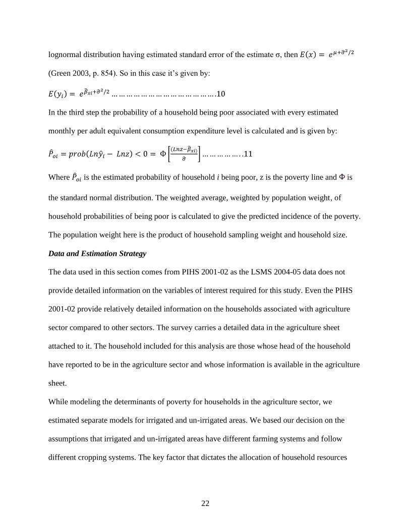
lognormal distribution having estimated standard error of the estimate σ, then
(Green 2003, p. 854). So in this case it‟s given by:
In the third step the probability of a household being poor associated with every estimated
monthly per adult equivalent consumption expenditure level is calculated and is given by:
Where is the estimated probability of household i being poor, z is the poverty line and is
the standard normal distribution. The weighted average, weighted by population weight, of
household probabilities of being poor is calculated to give the predicted incidence of the poverty.
The population weight here is the product of household sampling weight and household size.
Data and Estimation Strategy
The data used in this section comes from PIHS 2001-02 as the LSMS 2004-05 data does not
provide detailed information on the variables of interest required for this study. Even the PIHS
2001-02 provide relatively detailed information on the households associated with agriculture
sector compared to other sectors. The survey carries a detailed data in the agriculture sheet
attached to it. The household included for this analysis are those whose head of the household
have reported to be in the agriculture sector and whose information is available in the agriculture
sheet.
While modeling the determinants of poverty for households in the agriculture sector, we
estimated separate models for irrigated and un-irrigated areas. We based our decision on the
assumptions that irrigated and un-irrigated areas have different farming systems and follow
different cropping systems. The key factor that dictates the allocation of household resources

23
towards different farm and non-farm enterprises is the availability or the absence of irrigation
water.
Description of the explanatory variables
We group the potential explanatory variables into the following headings: demographic,
education, employment, agriculture specific physical assets and infrastructure. A key rule in
selecting potential explanatory variables is that they are exogenous to the current consumption
expenditure which is taken as dependent variable. For example the value of crop and livestock
produce, education expenditure or dwelling characteristics are not included because its value as
such or in the form of imputed value is already included into the consumption expenditure.
Under the demography we included variables related to household size (the number of members
in household), number of household members below 10 years of age, number of household
members above 60 years of age and age of the household head.
Education variables include variables on number of schooling years of the head of the household,
number of schooling years of spouse of household head and average schooling years of the
household that include all those members of the household who are above 18 years of age and
have completed their education and not pursuing any more schooling. Those household members
who are 18 years and above and still going to school were excluded because their expenditure on
schooling has been included in the dependent variable.
Four variables are included in the employment and income variables. Two dummy variables
were included related to remittances, one for household receiving these from within Pakistan and
one for receiving remittances from abroad. As all the households in the sample are those whose
head of the household is in agriculture sector, so two variables relating to employment of second
or additional member of the household were created. One variable include the number of

24
household members who are 18 years and above and are working in the agriculture or
construction or transport and communication industry. These three industries were grouped
together as the estimated average monthly per adult equivalent expenditure in these sectors was
less than the national average. The other variable includes the number of household members
employed in other industries. All other sectors, except the three mentioned earlier, were grouped
together as the estimated monthly per adult consumption expenditure in these sectors was more
than the national average.
Three agriculture specific variables related to physical assets were separately included. One
variable is related to the amount of land ownership in acres. Since because of the skewed nature
of the land distribution, households having more land usually do not cultivate all their land and
in some cases they are absentee landlords who do not cultivate their land or a portion of it at all.
In such cases the land is cultivated by tenants or share cropper or rent in by those who are
interested in cultivation but do not have land or sufficient land to do so. Keeping this in mind we
also included another variable that is related to amount of land cultivated (in acres) by those who
are tenants, share croppers and those whom rent in land for such purpose. The third variable in
this group is related to livestock. The data in the agriculture sheet in the PIHS 2001-02 provides
information on the value of livestock including cattle, buffaloes, sheep and goats, camels, horses
and donkeys . The information in this shape is of little use since we are interested in the marginal
contribution of a unit of a livestock to the dependent variable. A dummy variable for livestock is
also not a solution for this as different types of livestock are simply not comparable. A separate
dummy variable for every kind of livestock was also not feasible as in some cases one household
is having different kinds of animals. In such a scenario we made an arbitrary decision, though on
the expert opinion of some who work in the livestock market, by setting the price of an average
25
cow to Rs 25000/- per head. We then divided the value of cows by this price and got the units
(numbers) for it. We then converted the respective values for all kinds of animals accordingly
and termed this unit as Livestock Equivalent Unit (LSEU). For example, a buffalo with a value
of Rs 37500/- is equal to 1.5 LSEU and four goats worth Rs 25000/- is 1 LSEU. Apart from this,
it has an additional advantage of capturing quality difference within the same type of animals.
For instance a very good quality cow worth Rs 50000/- is two times LSEU. Additionally and
more importantly it helped in keeping the model parsimony by having more information in just
one variable.
One variable, the infrastructure index, is also included. This variable is a composite index of
access to the following facilities: electricity, natural gas (fuel), paved road and; market, bank,
fertilizer depot and tractor rental within the locality. We made a simple assumption by assigning
a weight of one to every facility and then taking its average for every household.
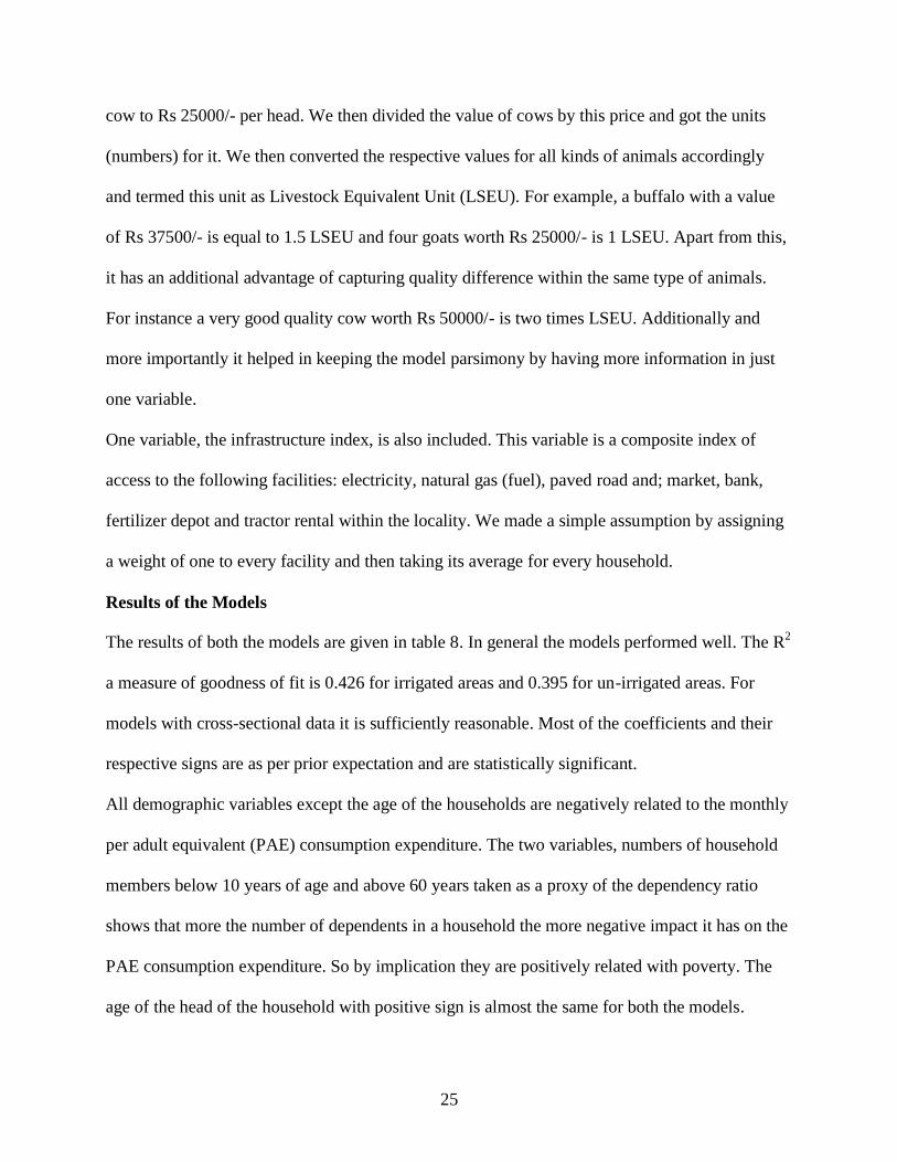
Results of the Models
The results of both the models are given in table 8. In general the models performed well. The R2
a measure of goodness of fit is 0.426 for irrigated areas and 0.395 for un-irrigated areas. For
models with cross-sectional data it is sufficiently reasonable. Most of the coefficients and their
respective signs are as per prior expectation and are statistically significant.
All demographic variables except the age of the households are negatively related to the monthly
per adult equivalent (PAE) consumption expenditure. The two variables, numbers of household
members below 10 years of age and above 60 years taken as a proxy of the dependency ratio
shows that more the number of dependents in a household the more negative impact it has on the
PAE consumption expenditure. So by implication they are positively related with poverty. The
age of the head of the household with positive sign is almost the same for both the models.

26
In the education variables, the schooling year of the household head is only significant for
irrigated areas while for un-irrigated areas it turns out to be insignificant. A possible reason for
this may the individuals with a little bit education background prefer to be out of the agriculture
sector especially in the un-irrigated areas. The other two variables have almost the same effect.
In the agriculture related variables, land ownership and livestock turned out to be significant for
both areas. As expected the gains from an extra unit of land (acre) in irrigated areas is more than
3.5 times that of un-irrigated areas. Because of the importance of the livestock in un-irrigated
areas its marginal contribution is greater in these areas compared to irrigated areas. The
cultivated land variable (the variable that include land cultivated by tenants, sharecroppers etc) is
not significant in the un-irrigated areas.
Other variables that contribute significantly to the household consumption are remittances from
abroad and the infrastructure index. The remittances from within the country have no significant
effect on the consumption. The reason for this may be that these household members do not have
sufficient skills or the resources to either go abroad or to participate effectively in the local
market. The insignificance of this variable also suggests low market demand for unskilled labor
that is evident in the form of low wage rate prevailing in the country. The significance of the
infrastructure index suggests that those households who have enough access to various facilities
tend to increase their welfare. It also suggest more investment on the part of the government in
this area as it happen to be the only area where the policy makers can make an influence
relatively easier compared to targeting other potential factors highlighted earlier.
Potential policy simulations
Table 9 shows the results of various policy simulations done with both models. The simulation
results are shown in terms of percentage change in the PAE consumption expenditure and

27
percentage change in head count index. The simulations results were compared with a base
simulation results that were estimated based on the parameters of the models for both the models.
Simulation 1 deals with increasing land of households who are already owners. We did not
assume redistribution which is rather an impractical scenario as the Pakistan has a background of
various failed land reforms since its inception. The increase of land by 1 acre also looks
impractical that without redistribution how it can be increased? We looked at it from another
perspective, from the perspective of increasing the productivity of land. If five acres of land are
made productive enough to produce equivalent of six acres so, at least, theoretically it got
increased by one acre. The simulation result shows that 1 acre of land increases the PAE
consumption by 5.24 percent and 2.31 percent in irrigated and un-irrigated areas respectively. It
decreases the head-count index by 6.23 percent and 2.83 percent in these households
accordingly. The result of increasing livestock unit by one is more pronounce in un-irrigated
households than irrigated ones for both consumption and head-count index. Simulation 3 is
related to increasing the mean schooling years of households with 18 years and above members
by 1 year. The results are somewhat the same for both irrigated and un-irrigated households. In
simulation 4 we increased infrastructure index by one unit for those households who were atleast
deficient on access to any one component of the infrastructure index. For un-irrigated households
the impact on both consumption and incidence on poverty is the maximum whereas for irrigated
households its second only to increase in the land ownership.
Conclusion
Our results for the incidence of absolute poverty in Pakistan show that for LSMS 2004-05 the
figures provided by the government are bit under estimated. We pointed out the reason for it
being the inflation of the base poverty line by the CPI which is an urban based index. We

28
inflated the base poverty line by the TPI, a survey based index and the results showed that the
decrease in incidence of poverty is almost half as reported in official documents. Our results
support the poverty growth nexus but also pointed out that the benefit of the growth was reaped
more by those who were already rich and showed the worsening of the consumption expenditure
inequality over time.
Overall poverty is concentrated more in rural areas and agriculture sector contributes more to the
national poverty as compared to other sectors. The monthly average per adult equivalent
consumption expenditure is lower for all quintiles of the agriculture sector compared to the
national averages for both the surveys. Any effort to alleviate poverty in Pakistan needs a
focused attention to this sector because of the bulk of the population attached to this sector and
the reliance of other sectors on it through backward and forward linkages.
The results indicate the importance of investment in increasing the productivity of land and
livestock to help people in poverty in the agriculture sector and to invest in infrastructure for
overall decrease in poverty.

29
References
Atkinson, A.B. 1989. “Poverty”. In Social economics: The New Palgrave, ed. J. Eatwell, M.
Milgate, and P. Newman, NewYork: Norton.
Cheema, I.A. 2005. “A Profile of Poverty in Pakistan”. Centre For Research On Poverty Reduction And
Income Distribution Islamabad www.crprid.org .
CRPRID. 2002. “ Pakistan Human Condition Report”. Centre for Research on Poverty Reduction and
Income Distribution, Pak Secretariat, Islamabad.
_______ 2002. “Issues in Measuring Poverty in Pakistan”. Centre for Research on Poverty Reduction and
Income Distribution, Pak Secretariat, Islamabad.
Datt, G. and D. Jolliffe. 2005. “Poverty in Eygpt: Modeling and Poverty Simulations”.
Economic Development and Cultural Change. 53(2): 327-346.
Deaton, A. and A. Tarozzi. 2000. ”Prices and Poverty in India”. Princeton, New Jersey:
Princeton University, Program in Development Studies. Available:
www.wws.princeton.edu:80/rpds/working.htm
Deaton, A. and S. Zaidi. 2002. “Guidelines for Constructing Consumption Aggregates for
Welfare Analysis”. Living Standards Measurement Study, Working Paper No. 135.
World Bank Washington DC.
Fagernas, S. and L. Wallace. 2007. “Determinants of Poverty in Sierra Leone, 2003”. ESAU
Working Paper 19. Overseas Development Institute London. March.
FAO 2004. The State of Food Insecurity in the World 2004. Food and Agriculture Organization
of the United Nations, Rome, Italy.
_____ 2004a. Socio-economic Analysis and Policy Implications of the Roles of Agriculture in
Developing Countries Research Program. Summary Report 2004. Food and Agriculture
Organization of the United Nations, Rome, Italy.
_____2005. The State of Food and Agriculture: Agricultural Trade and Poverty. FAOAgriculture
Series No.36. Food and Agriculture Organization of the United Nations, Rome.

30
Foster, J., J. Greer, and E. Thorbecke. 1984. “A Class of Decomposable Poverty
Measures”. Econometrica 52(3): 761-766.
Gibson, J. and S. Rozelle. 2003. “Poverty and Access to Roads in Papua New Guinea”.
Economic Development and Cultural Change. 52(1):159-185.
Government of Pakistan. 2002. Planning and Development Division‟s notification
No.1(41)Poverty/PC/2002 dated 16 August 2002.
___________________ 2004-05. Economic Survey of Pakistan. Economic Advisor's Wing.
Finance Division, Islamabad.
__________________2008. http://statpak.gov.pk/depts/fbs/statistics/price_statisti. Source:
Visited March 18 2008.
Greene, W. H. 2003. “Econometrics Analysis”. Fifth Edition, Prentice Hall New York.
Human Development Report. 2007. UNDP www.hdr.undp.org/en/reports/global/hdr2007-2008
Jamal, H. 2004. “In Search of Poverty Predictors: The case of Urban and Rural Pakistan”.
Report No. 59. Social Policy Development Institute (SDPI), Islamabad, Pakistan.
December.
Kakwani, N.2003. “Issues in Setting Absolute Poverty Lines”, Poverty and Social Development
Paper No. 4, ADB, Manila.
Malik, S. J. 2005. “Agricultural Growth and Rural Poverty: A Review of Evidence”.
Working Paper No. 2. Pakistan Resident Mission, Asian Development Bank.
Pasha, H. A. and T. Palanivel. 2003. “Macroeconomics of Poverty Reduction: An Analysis of
the Experience in 11 Asian Countries” Discussion Paper No. 3, UNDP Asia-Pacific
Regional Programme on Macroeconomics of Poverty Reduction.
Ravallian, M. 1992.“ Poverty Comparisons: A Guide to Concepts and Methods”, LSMS
Working Paper No. 88. The World Bank.
31
___________. 1996. “Issues in Measuring and Modeling Poverty”. The Economic Journal.
106(438):1328-1343.
Ravallion, M. and B. Bidani. 1994. “How Robust is a Poverty Profile?” World Bank
Economic Review 8: 75-102. Washington D.C.: The World Bank.
Simler, R. K., S. Mukerjee, G. L. Dava and G. Datt. 2004. “Rebuilding After War: Micro-level
Determinants of Poverty Reduction In Mozambique”. Report No. 132. IFPRI,
Washington, DC.
UNDP. 2007. “Pakistan Millennium Development Goals Report”. United Nations Development
Program, Islamabad.
World Bank. 2006. www.siteresources.worldbank.org/PovertyHCR2000-2005.pdf
________. 2005. “Introduction to Poverty Analysis”. World Bank Institute, Washington DC.
August.

32
Table 1. Households included in the study
Province/
Region
PIHS 2001-02 LSMS 2004-05
Urban Rural Total Urban Rural Total
Punjab 2542 3768 6310 2510 3605 6115
Sind 1533 2173 3706 1497 1980 3477
NWFP 840 1825 2665 1087 1878 2965
Baluchistan 621 1403 2024 713 1434 2147
Total 5536 9169 14705 5807 8897 14704
Table 2. Inflation Rate Based on Tranqvist Price Index (TPI)
Region HH Weight*
TPI Weighted TPI
Punjab - Urban 0.176 26.858 4.733
Rural 0.412 31.401 12.948
Sind - Urban 0.105 18.793 1.970
Rural 0.141 26.106 3.669
NWFP – Urban 0.019 25.578 0.495
Rural 0.105 28.101 2.939
Baluchistan - Urban 0.008 32.526 0.2479
Rural 0.035 39.479 1.363
Inflation (%) 28.365
*HH Weight shows the share of households represented by the region in over-all sample

33
Table 3. Comparison of Poverty Estimates (PIHS 2001-02 and LSMS 2004-05)
Region /
Sector
Poverty Estimates
Head Count Poverty Gap Severity of Poverty
2001-02 2004-05 2001-02 2004-05 2001-02 2004-05
Urban 23.56 19.08 4.73 3.77 1.42 1.15
Rural 40.29 34.62 8.35 7.28 2.56 2.34
Total 35.44 29.70 7.30 6.17 2.23 1.96
Agriculture 39.10 31.90 8.02 6.58 2.43 2.14
Table 4. Real Growth Rates*
Year Over all Agriculture
2000-01 2 -2.2
2001-02 3.1 0.1
2002-03 4.7 4.1
2003-04 7.5 2.4
2004-05 9 6.5
*GDP at Factor Cost
Source: Economic Survey (2006-07), Government of Pakistan.

34
Table 5. Mean Monthly Per Adult Equivalent Consumption Expenditure (Rs)
Expenditure
Quintile
Overall Agriculture Sector
PIHS-
2001
LSMS-2004-05
(2001-02
Prices) %Change
PIHS-
2001
LSMS-2004-
05 (2001-02
Prices) %Change
Poorest 20% 507.40 524.85 3.44 506.62 519.54 2.34
2 690.31 733.24 6.21 689.30 728.46 5.37
3 845.36 909.34 7.56 844.50 904.46 6.72
4 1070.14 1171.90 9.51 1069.06 1162.56 8.74
Richest 20% 1907.34 2207.90 15.75 1706.96 2012.27 17.90
Overall 1004.20 1109.51 10.50 916.80 1006.73 9.80

35
Table 6. Contribution to Overall Poverty by Region and Sectors
Region/Industry
2001-02 2004-05
Percent
Contribution
Pop*
Share
Concen.
Index**
Percent
Contribution
Pop
Share
Concen.
Index
Poor Non-Poor Poor Non-Poor
Region 19.25 34.28 28.95 0.66 20.4 36.52 31.73 0.64
Urban 80.75 65.72 71.05 1.14 79.6 65.48 68.27 1.17
Rural 35.44 64.56 100 0.35 29.7 70.3 100 0.30
Industry/Sector
Agriculture, Livestock 44.39 38.26 40.44 1.10 40.24 35.89 37.18 1.08
Mining and Manufacturing 8.11 8.91 8.63 0.94 7.89 8.14 8.07 0.98
Electricity, water and gas 0.79 1.46 1.22 0.65 0.49 1.04 0.88 0.56
Construction 13.19 5.68 8.35 1.58 10.27 5.89 7.18 1.43
Wholesale, retail, restaurant 11.46 16.03 14.41 0.80 13.27 18.22 16.76 0.79
Transport and
communication 6.46 6.65 6.58 0.98 5.37 5.47 5.44 0.98
Finance, Insurance, Real
Estate 0.18 1.08 0.76 0.23 0.15 0.56 0.54 0.27
Community and personal
services 13.87 19.10 17.24 0.80 18.07 19.92 19.37 0.93
Not adequately defined 1.56 2.83 2.38 0.66 4.25 4.87 4.69 0.90
*Population Share
**Concentration Index

36
Table 7. Descriptive Statistics
Variable
Irrigated
(N= 2578) Un-irrigated
(N=1706)
Mean SD Mean SD
Log: Monthly Per Adult Equivalent
Expenditure 6.858 0.430 6.727 0.406
Dummy Sind 0.260 0.440 0.239 0.427
Dummy NWFP 0.080 0.270 0.160 0.366
Dummy Baluchistan 0.030 0.175 0.060 0.238
Dummy Urban 0.030 0.183 0.053 0.223
HH size 7.530 3.485 6.697 3.168
Number of members below 10 years of
age 2.255 1.944 2.119 1.845
Number of members age 60 and above 0.502 0.699 0.440 0.662
Age of HH head 45.550 13.567 45.308 13.751
Household Head's Schooling years 2.406 3.554 1.675 3.112
Number of Schooling Years of Spouse of
HH head 0.354 1.541 0.226 1.160
Average Schooling Years of HH 4.222 3.685 3.218 3.638
Log: Land Owned 1.745 2.915 2.13 2.786
Log: Cultivated Land 1.042 2.886 1.01 1.02
Livestock cattle-head equivalent unit
(LSEU) 1.613 1.993 0.926 1.403
No. of HH members employed in agri.,
construction and Transport 1.756 1.832 1.209 1.423
No. of HH members employed in other
sectors 0.170 0.501 0.175 0.522
Dummy: Remittances from within country 0.070 0.262 0.137 0.344
Dummy: Remittances from Abroad 0.020 0.130 0.030 0.171
Infrastructure Index 0.375 0.175 0.347 0.225

37
Table 8. OLS Estimates of the Model of Log Per Adult Equivalent Consumption
VARIABLE Irrigated Un-Irrigated
NAME COEFFICIENT t-Ratio COEFFICIENT t-Ratio
HH size -0.030 -6.36 -0.049 -8.36
Number of members below 10
years of age -0.042 -6.24 -0.033 -4.00
Number of members age 60 and
above -0.032 -2.65 -0.032 -2.14
Age of HH head 0.002 3.15 0.002 2.79
Household Head's Schooling
years 0.016 6.60 0.004 1.06
Number of Schooling Years of
Spouse of HH head 0.027 4.64 0.026 3.07
Average Schooling Years of HH 0.121 2.89 0.011 3.06
Log: Land Owned 0.103 10.02 0.028 6.89
Log: Cultivated Land 0.077 7.58 0.005 0.72
Livestock cattle-head equivalent
unit (LSEU) 0.037 4.67 0.043 5.54
No. of HH members employed in
agri., construction and Transport -0.031 -5.59 -0.022 -2.94
No. of HH members employed in
other sectors 0.055 3.26 0.018 1.07
Dummy: Remittances from
within country 0.061 1.71 0.017 0.59
Dummy: Remittances from
Abroad 0.282 4.77 0.230 5.18
Infrastructure Index 0.104 2.02 0.185 2.83
CONSTANT 7.243 122.90 6.962 121.20
R2
0.426 0.395

38
Table 9. Potential Simulations (% change over base simulations)
Simulation
Irrigated Un-irrigated
Mean
Consumption
Head-Count
index
Mean
Consumption
Head-Count
index
Increasing Land by 1 acre 5.24 -6.23 2.31 -2.83
Increasing LSEU by 1 unit 2.81 -3.21 3.33 -4.15
Increasing Mean Schooling Years
by I year 2.12 -2.89 2.21 -3.12
Increasing Infrastructure Index
by 1 Unit 4.75 -6.13 5.76 -6.87