Genetic Epidemiology 34 : 434–443 (2010)

An ‘‘Almost Exhaustive’’ Search-Based Sequential PermutationMethod for Detecting Epistasis in Disease Association Studies

Li Ma,1 Themistocles L. Assimes,2 Narges B. Asadi,3 Carlos Iribarren,4 Thomas Quertermous,2

and Wing H. Wong1,5�

1Department of Statistics, Stanford University, Stanford, California2Department of Medicine, Stanford University, Stanford, California

3Department of Electrical Engineering, Stanford University, Stanford, California4Division of Research, Kaiser Permanente, Oakland, California

5Department of Health Research and Policy, Stanford University, Stanford, California

Due to the complex nature of common diseases, their etiology is likely to involve ‘‘uncommon but strong’’ (UBS) interactiveeffects—i.e. allelic combinations that are each present in only a small fraction of the patients but associated with highdisease risk. However, the identification of such effects using standard methods for testing association can be difficult. Inthis work, we introduce a method for testing interactions that is particularly powerful in detecting UBS effects. The methodconsists of two modules—one is a pattern counting algorithm designed for efficiently evaluating the risk significance ofeach marker combination, and the other is a sequential permutation scheme for multiple testing correction. We demonstratethe work of our method using a candidate gene data set for cardiovascular and coronary diseases with an injected UBSthree-locus interaction. In addition, we investigate the power and false rejection properties of our method using data setssimulated from a joint dominance three-locus model that gives rise to UBS interactive effects. The results show that ourmethod can be much more powerful than standard approaches such as trend test and multifactor dimensionality reductionfor detecting UBS interactions. Genet. Epidemiol. 34 : 434–443, 2010. r 2010 Wiley-Liss, Inc.

Key words: genetic interaction; nonparametric test; case-control study; frequent-pattern mining

Contract grant sponsor: NIH; Contract grant number: R01-HG004634; Contract grant sponsor: NSF; Contract grant numbers: DMS-0906044; DMS-0821823.�Correspondence to: Wing H. Wong, 390 Serra Mall, Stanford, CA 94305. E-mail: whwong@stanford.eduReceived 15 October 2009; Revised 17 December 2009; Accepted 17 January 2010Published online 25 June 2010 in Wiley InterScience (www.interscience.wiley.com).DOI: 10.1002/gepi.20496

INTRODUCTION

Epistasis has long been suspected to contribute to theunexplained genetic variance of common complex traits[Maher, 2008; Moore and Williams, 2009], and manystatistical methods have been proposed in recent years toidentify genetic interactions. Some notable examplesinclude multifactor dimensionality reduction (MDR) [Bushet al., 2006; Moore and Williams, 2009; Ritchie et al., 2001],random forests [Lunetta et al., 2004], and Bayesianepistasis association mapping [Zhang and Liu, 2007].(Interested readers can see [Cordell, 2009] for a review ofthese and other existing approaches.) While these methodshave led to some interesting findings of genetic inter-action, their application to common diseases, so far, hasachieved limited success.

The performance of most existing methods for testingdisease association rely on an implicit assumption that theunderlying allelic combinations of interest contribute tothe disease risk of a large proportion of the patients.However, for common diseases, whose etiology involvesmultiple biological pathways and is influenced by variousenvironmental factors, it is very likely that there exist

allelic combinations that are present in only a smallfraction of the patients, but when present, incur highdisease risk. For example, a particular allelic combinationmay have a disease risk ratio as high as 4, but is present inonly 10% of the patients. For simplicity we refer to these as‘‘uncommon but strong’’ (UBS) effects. A considerable partof the missing inheritability of common diseases could bedue to such effects.

Because each ‘‘uncommon’’ effect pertains to only asmall fraction of patients, they often do not exhibit maineffects significant enough to withstand multiple testingcorrection. Thus, methods that rely on recovering interac-tions from significant marginal effects are not effective indetecting UBS effects. One way to overcome this difficultyis to test marker combinations directly in an exhaustivemanner. Some existing methods such as MDR indeedadopt this exhaustive search scheme.

When using an exhaustive search scheme to look forinteractions (not just UBS effects but interactions ingeneral), one must be careful about how statisticalinference, in particular multiple testing correction, shouldbe carried out. More specifically, multiple testing correc-tion methods such as permutation testing must beadjusted in two important ways for this context. First,

r 2010 Wiley-Liss, Inc.

correction should be done conditional on the length ofthe interactions (i.e. the number of markers involved) inthat the space of all possible marker combinations expandrapidly with their length. Second, in ‘‘correcting’’ thep-value of any marker combination, the effects of itssub-combinations should be taken into account. These twopoints have mostly been ignored in existing methodsbased on exhaustive search. In our later simulationstudies, we will demonstrate that this could severelyjeopardize the power for detecting interactions.

In this work, we propose a method for testing epistasisthat is particularly powerful in detecting UBS effects. Themethod follows the exhaustive search scheme, butachieves high computational efficiency by skipping inthe search procedure parts of the marker combinationspace that cannot contain detectable signals. (Hence it is‘‘almost’’ exhaustive.) In addition, it adopts a sequentialpermutation procedure for multiple testing correction thataddresses the two issues mentioned in the previousparagraph. We demonstrate the work of our method in acardiovascular disease candidate gene study data set withan injected UBS signal. Also, we study the power and falserejection properties of the method using data setssimulated from a three-locus joint dominance model thatgives rise to UBS interactive effects.

METHODS

BASIC TERMINOLOGY

We first introduce some basic terms that will be usedthroughout the rest of the paper. A genetic pattern(or pattern for short) is defined to be a combination ofmarker-genotypes, and we write them in parentheses. Forexample, (SNP3 5 C/G, SNP4 5 T/T, SNP7 5 A/T) is apattern involving three markers. We define the length of apattern as the number of genetic markers it involves. Sothe previous pattern is of length three. For simplicity,patterns of length k are called k-patterns. Next, we use‘‘marker combination’’ (corresponding to a pattern) tomean the set of markers involved in the pattern, and writethem in parentheses as well. For instance, (SNP3, SNP4,SNP7) is the corresponding marker combination for theprevious pattern. Lastly, the support of a pattern refers tothe relative frequency of the pattern among the observa-tions. For example, if 40 out of 1,000 cases and 60 out of 600controls have the pattern, then it is said to have a casesupport of 4% and a control support of 10%, as well as anoverall support of 6.25%.

EVALUATING THE SIGNIFICANCE OFGENETIC PATTERNS

The simplest way to evaluate the disease association ofall possible genetic patterns is to conduct an exhaustivesearch over the space of all possible patterns up to a givenlength. However, such an approach wastes a lot ofcomputational power on patterns that occur so rarelyamong the subjects that even a 100% observed penetrancewould not render a p-value significant enough to survivemultiple testing correction. For example, suppose a3-pattern occurs only 1% of the time in a data set of1,000 cases and 1,000 controls with 600 candidate markers.Even if all of the subjects having this pattern had thedisease, corresponding to a nominal p-value of about 10�3,

this would still not be sufficient evidence to establish anassociation between this pattern and the disease risk.Therefore, one loses little power by excluding suchinfrequent patterns in the search for interactions.

Interestingly, making the seeming compromise of leav-ing the infrequent part of the space of genetic patterns outof the search opens a door to a class of very efficient searchalgorithms developed in the machine learning literature—the so-called frequent-pattern mining algorithms. In theoriginal frequent-pattern mining setting that motivatedthe development of those algorithms, the data set isunsupervised, i.e., without a case label, and the goal is tofind and count all patterns whose support is above agiven threshold, say 2%, among all observations. (Thesepatterns are termed the ‘‘frequent patterns.’’) The algo-rithms accomplish this task by utilizing advanced datastructures which drastically expedites the search-and-count procedure.

Our current problem of searching for genetic patternsassociated with a disease label is slightly more compli-cated than the standard frequent-pattern mining problem.First, given a case label, we want to find those frequentgenetic patterns and count them among the cases and thecontrols separately. (With these two counts, we can thenapply tests, e.g. Fisher’s exact test, to evaluate thesignificance of support difference between cases andcontrols.) Another difference is that we want to select thefrequent patterns based on their support in either the casesalone or the controls alone rather than based on theiroverall support. This will allow us to capture thosepatterns that are infrequent overall but frequent amongone of the two groups.

Despite these differences, frequent-pattern mining algo-rithms, with some minor changes, can be applied in ourcontext for testing epistasis. We adopt one of the fastestsuch algorithms, FP-growth [Borgelt, 2005; Han et al.,2004] for this purpose. (‘‘FP’’ stands for frequent pattern.)We extended the algorithm to serve our current contextand call the new version ‘‘supervised FP-growth’’ toemphasize its key difference from the original version.(See the ‘‘Software’’ section for more information.) In short,the supervised version takes two arguments n and s, andfinds all patterns of length up to n whose case support isabove s. In addition, it counts each such pattern amongcases and controls separately. (Note that by specifying athreshold on the case support instead of the total support,we allow patterns with very low control support to stay inour search space. This leads to the preferential discovery ofpatterns that increase disease risk. To detect patterns thatdecrease the risk of disease, we can simply reverse thecase/control label.)

With the case and control counts for each frequentgenetic pattern, we can apply any one degree of freedomtest to measure the significance of its association withdisease risk. In this study we use Fisher’s exact test. Weacknowledge that 1-d.f. tests are not the most powerful inthat they do not combine information across patternsinvolving the same markers. However such tests areextremely attractive computationally in the current setting.Because for any given data set, a pattern’s p-value undersuch a test depends only on its case and control counts, agrid of p-values corresponding to all possible combina-tions of case and control counts can be precomputed. Eachfrequent pattern found by supervised FP-growth can thenbe directly mapped to the corresponding p-value on the

435A Sequential Method for Testing Epistasis

Genet. Epidemiol.

grid without being tested on-the-fly. This raises computa-tional efficiency greatly especially when a huge number ofpatterns are being tested.

MULTIPLE TESTING CORRECTION

Supervised FP-growth provides a means to measure thestatistical significance of disease association for individualgenetic patterns. While the p-values it generates can serveto rank the patterns in terms of their statistical signi-ficance, they cannot be taken at face value due to the largenumber of tests conducted. In fact, the multiple testingproblem is much more serious in the current settingof testing interactions compared to testing main effectsbecause the number of marker combinations is muchlarger than the number of markers. A common solution tothe problem is to use permutation testing.

The appropriate permutation procedure for our pro-blem, however, deviates in two important ways from thestandard permutation test. First, p-values for the patternsof different lengths should be tested separately, i.e., usingdifferent permutation nulls. As the number of patternsincreases combinatorially with their length, there areorders of magnitude more long patterns than shortones. Hence, small p-values are much more likely toappear among longer patterns. If a common permutationnull were used for patterns of all lengths, the effect of, say,2-patterns would be ‘‘masked’’ by the noise of 3-patterns.This problem is amplified as the length of patterns underinvestigation increases. Second, as we conduct separatepermutation testing for patterns of different lengths, thepermutation nulls for longer patterns should take intoaccount the significant effects detected among the shorterones. For example, if a marker combination (SNP1, SNP2)has been determined to be strongly associated with thedisease risk, then many 3-patterns that contain this markercombination may also display significant, or even moresignificant, p-values just due to chance. Those will showup as significant 3-patterns while their effect is, in fact,already accounted for by a subset of the markers theyinvolve. More generally, if the effect of a marker combina-tion can be explained by one or more of itssub-combinations, then we should try to recover suchsub-combinations rather than declare the longer onesignificant. Thus, the significant patterns of length up ton�1 should be considered in constructing the nullhypotheses for n-patterns. Our reasoning here is analogousto that used in forward stagewise model selection in theregression setting. In that setting, if certain marginal effectsare determined to be significant, one compares anexpanded model to the already established model insteadof the empty model.

For these reasons we propose a sequential permutationtesting procedure. The basic idea is to test the 1-patternsfirst followed by the 2-patterns using the effects detectedin the 1-patterns as the null, and then test the 3-patternsusing the effects detected in the 1-patterns and 2-patternsas the null, and so on and so forth. Next we describe thissequential procedure, which we call adaptive marginaleffect permutation (AMEP) in an inductive manner.

Suppose we have completed our testing for patterns oflength up to n�1, and have arrived at a set, Sn�1,of significant marker combinations up to length n�1.(A marker combination is called significant if one of itscorresponding genetic patterns is significant.) To test the

n-patterns, we first divide them into G groups in such afashion that the patterns within each group share exactlythe same set of significant marker combinations. The idea isto construct a separate permutation null for each of the Ggroups. (Note that G depends on both n and Sn�1. To bemost precise, we can write G as Gðn; Sn�1Þ.) For example,suppose we have tested the 1-patterns and have found twosignificant markers, S1 ¼ fðSNP2Þ; ðSNP5Þg. In testing the 2-patterns, we divide them into G 5 4 groups—(G1) those thatdo not contain either SNP2 or SNP5, (G2) those containingSNP2 but not SNP5, (G3) those containing SNP5 but notSNP2, and (G4) those containing both SNP2 and SNP5.

The G permutation nulls, one for each of the G groups, canbe constructed simultaneously by permuting the case labeltogether with all the markers in Sn�1. For each permutation,we apply the supervised FP-growth algorithm just as we didfor the original data. By pooling the p-values of the patternsbelonging to each of the G groups from all the permutations,we obtain a sample of p-values from the permutation nullfor each of the G groups. The corrected p-value for a patterncan then be computed as the proportion of permutationsthat generated a more significant p-value in the correspond-ing group. Those patterns whose corrected p-values pass asignificance threshold, e.g. 5%, are declared as significant,and their corresponding marker combinations are joinedwith Sn�1 to form Sn. A formal algorithm-style description ofAMEP is provided in Box 1.

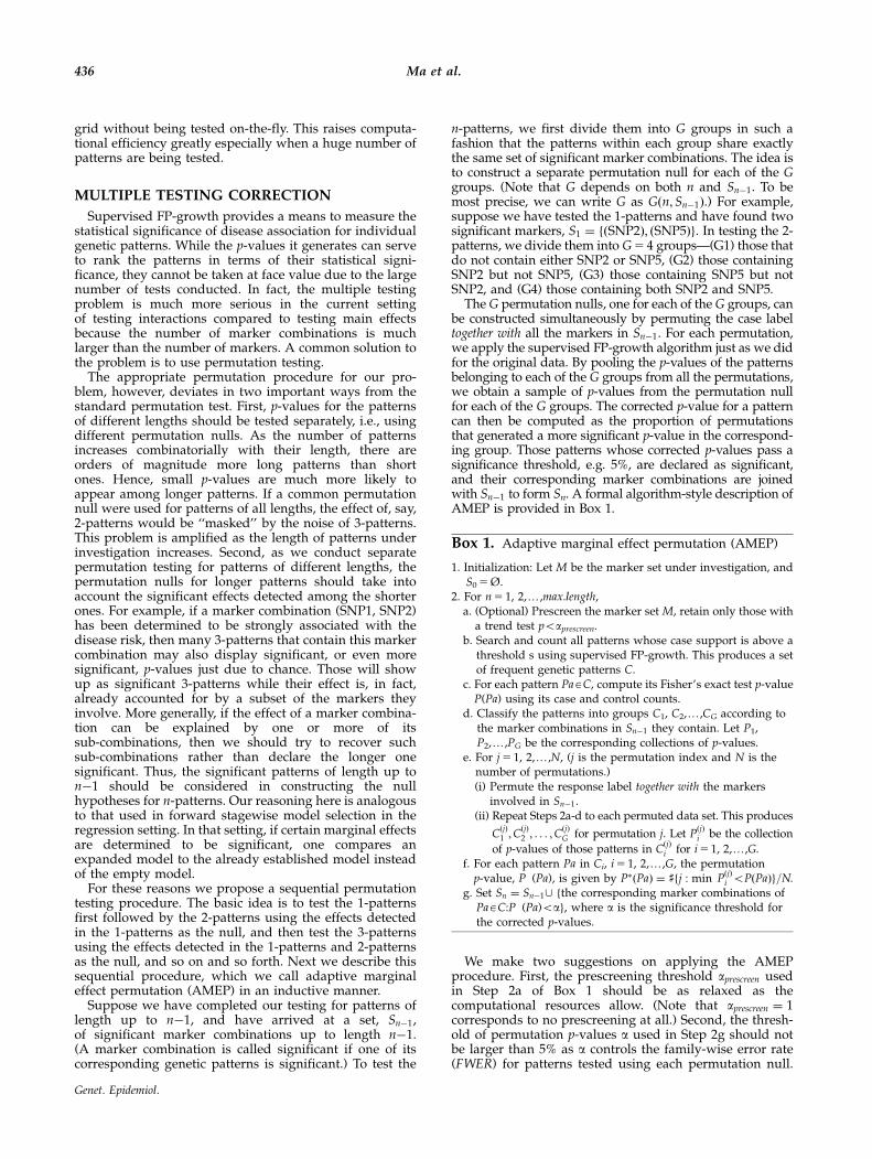
Box 1. Adaptive marginal effect permutation (AMEP)

1. Initialization: Let M be the marker set under investigation, andS0 5 Ø.

2. For n 5 1, 2,y,max.length,a. (Optional) Prescreen the marker set M, retain only those with

a trend test poaprescreen.b. Search and count all patterns whose case support is above a

threshold s using supervised FP-growth. This produces a setof frequent genetic patterns C.

c. For each pattern PaAC, compute its Fisher’s exact test p-valueP(Pa) using its case and control counts.

d. Classify the patterns into groups C1, C2,y,CG according tothe marker combinations in Sn�1 they contain. Let P1,P2,y,PG be the corresponding collections of p-values.

e. For j 5 1, 2,y,N, (j is the permutation index and N is thenumber of permutations.)(i) Permute the response label together with the markers

involved in Sn�1.(ii) Repeat Steps 2a-d to each permuted data set. This produces

CðjÞ1 ;C

ðjÞ2 ; . . . ;C

ðjÞG for permutation j. Let P

ðjÞi be the collection

of p-values of those patterns in CðjÞi for i 5 1, 2,y,G.

f. For each pattern Pa in Ci, i 5 1, 2,y,G, the permutationp-value, P�(Pa), is given by P�ðPaÞ ¼ ]fj : min P

ðjÞi oPðPaÞg=N.

g. Set Sn ¼ Sn�1[ fthe corresponding marker combinations ofPaAC:P�(Pa)oag, where a is the significance threshold forthe corrected p-values.

We make two suggestions on applying the AMEPprocedure. First, the prescreening threshold aprescreen usedin Step 2a of Box 1 should be as relaxed as thecomputational resources allow. (Note that aprescreen ¼ 1corresponds to no prescreening at all.) Second, the thresh-old of permutation p-values a used in Step 2g should notbe larger than 5% as a controls the family-wise error rate(FWER) for patterns tested using each permutation null.

436 Ma et al.

Genet. Epidemiol.

While this criterion may appear stringent, we justify it onthe basis that significant patterns passing this thresholdaffect the null hypotheses for testing longer patterns. Weshould only allow patterns that demonstrate reasonablystrong evidence of association to affect the testing for otherpatterns.

On the other hand, however, those patterns withmoderately significant permutation p-values, though notpassing the 5% FWER threshold, may still be of interest.Such patterns should not serve in the permutation nulls forlonger patterns, but may still contain evidence for trueassociation. To find such patterns, we extend the AMEPprocedure by reporting, in addition to Sn, all patternswhose p-values pass less stringent p-value cutoffs con-structed based on controlling the number of false positives(NFP), or alternatively the false discovery rate (FDR). Thedetail of this extended procedure is presented in Box 2.

Box 2. Modified AMEP procedure for controlling NFPor FDR1. Initialization: Let M be the marker set under investigation, and

S0 5 |.2. For k 5 1, 2,y,max.length,

a-g. Same as the original AMEP procedure.h. Pool the patterns and their p-values from all the permutations

according to their classes.For iAf1, 2,y,Gg, let C

ðpooledÞi ¼ [N

j¼1CðjÞi , and

PðpooledÞi ¼ [N

j¼1PðjÞi .

i. For each Ci, PðpooledÞi gives the empirical permutation null

distribution of the Fisher’s p-values. Hence, the number of falsepositives (NFP) as a function of the p-value cutoff for Group ican be estimated as dNFPiðpÞ ¼ ]felements in P

ðpooledÞi � pg=N,

while the number of rejections in the original data isNPi ðpÞ ¼ ]felements in Pi � pg.

j. The corresponding estimated FDR is dFDRiðpÞ ¼ dNFPiðpÞ=NPi ðpÞ.k. A p-value cutoff pi can be chosen for permutation null group i

to control dNFPi or dFDRi.l. Report the patterns in each group whose p-values pass the

corresponding p-value cutoff pi.

In particular, Steps 2i and 2j in Box 2 show how one canestimate the NFP and FDR, as functions of the cutoffp-value, for each of the G n-pattern groups. In Step 2k weselect an appropriate p-value cutoff separately for eachgroup based on the estimated NFP or FDR. For example,one can choose the p-value cutoffs so that the estimatedNFP for each group is 0.2. We denote this particularp-value cutoff by pnfp0:2, which is group specific, and willuse it in the following data analytical example.

SIMULATION STUDIES

A REAL DATA SET WITH AN INJECTED UBSSIGNAL

We now demonstrate the work of our method using areal data set—namely the ADVANCE (AtheroscleroticDisease, VAscular function, and genetiC Epidemiology)study data—with an injected signal. ADVANCE is apopulation based case-control study with a primary aimof identifying novel genetic determinants of coronaryartery disease. Between October 28, 2001 and December 31,

2003, a total of 3,179 members of Kaiser Permanente ofNorthern California were recruited into 3 case cohorts and2 control cohorts [Assimes et al., 2008]. Case cohortsincluded members with clinically significant CAD (namelyangina, myocardial infarction, or a history of coronaryangioplasty or bypass procedures) while control cohortshad no history of clinical CAD. In Phase 1, a small numberof cases were sequenced at approximately 100 candidategenes and a subset of sequenced SNPs were thengenotyped in all participants. To avoid potential popula-tion stratification, we use only the European samples fromthe two older case cohorts and the older control cohorts.The data set consists of 580 SNP markers in 957 cases and677 controls. Each of the SNPs is assigned a name (e.g,ABC1_17) indicating its genomic location and correspond-ing gene. Interested readers can find the rs numbers for allthe SNPs as well as other information about the study athttp://med.stanford.edu/advance/.

We spike in a three-locus interaction by enforcing arandomly chosen pattern (ABC1_17 5 A/A, CNTNAP5_500 5 C/T, ANGPT1_R_3 5 T/T) to be associated with thedisease risk. The only criteria used in choosing this patternare that (1) its overall support is small, not exceeding 5%and (2) there is no evidence of association for the markersinvolved in the original data. We inject the signal byflipping the disease labels of 29 randomly chosen controlsin the original data that possess this genotypic pattern tocases. Before the flipping, 48 out of the 957 cases and36 out of the 677 controls had this pattern. After theflipping, 77 out of 986 cases and 7 out of 648 controls havethis pattern, corresponding to about 7.9% of the cases and1.1% of the controls. Note that this mimics a stronginteractive effect present in a small fraction of the cases, i.e.a UBS effect.

Before applying our method, we first check what thestandard approach, trend test, would reveal about thedata. The histogram of the trend test p-values given inFigure 1 shows that none of the three markers involved inour injected signal have a permutation corrected p-value ofless than 5% (based on 1,000 permutations). Thus, thestandard approach would discard all three at the singlemarker testing stage, leaving no hope for any follow-up

–log 10 p–value

Freq

uenc

y

0 1 2 3 4

02

46

810

ABC1_17

CNTNAP5_500

ANGPT1_R_3

Corrected 5% level

Fig. 1. A truncated histogram of the trend test �log10 p-values.The frequency (vertical axis) is truncated at 10. The dashed

vertical line indicates the permutation corrected 5% level. The

three markers involved in our injected signal fall into the bars

indicated by the red arrows.

437A Sequential Method for Testing Epistasis

Genet. Epidemiol.

analysis, such as fitting a logistic regression to thesignificant markers, to uncover the interactive effect.

To apply our method to the data, first we need to specifya few parameters. We set the (within case) supportthreshold for the supervised FP-growth algorithm s to 2%,and the prescreening threshold aprescreen to 0.2. (In fact, for adata set of this size the supervised FP-growth algorithm isefficient enough so that no screening is necessary at all forinvestigating interactions involving up to three markers.Here we apply prescreening to demonstrate our method atwork in general. See Discussions for more detail oncomputational efficiency.) We set N 5 5,000 as the numberof permutations for each pattern length. Finally, we use theconventional level 0.05 for the FWER threshold a, and adoptthe pnfp0:2 level as the p-value cutoff to control the estimatedNFP for each permutation null group.

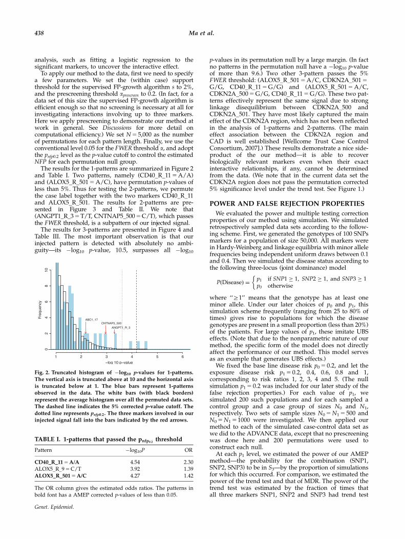
The results for the 1-patterns are summarized in Figure 2and Table I. Two patterns, namely (CD40_R_11 5 A/A)and (ALOX5_R_501 5 A/C), have permutation p-values ofless than 5%. Thus for testing the 2-patterns, we permutethe case label together with the two markers CD40_R_11and ALOX5_R_501. The results for 2-patterns are pre-sented in Figure 3 and Table II. We note that(ANGPT1_R_3 5 T/T, CNTNAP5_500 5 C/T), which passesthe FWER threshold, is a subpattern of our injected signal.

The results for 3-patterns are presented in Figure 4 andTable III. The most important observation is that ourinjected pattern is detected with absolutely no ambi-guity—its �log10 p-value, 10.5, surpasses all �log10

p-values in its permutation null by a large margin. (In factno patterns in the permutation null have a �log10 p-valueof more than 9.6.) Two other 3-pattern passes the 5%FWER threshold: (ALOX5_R_501 5 A/C, CDKN2A_501 5G/G, CD40_R_11 5 G/G) and (ALOX5_R_501 5 A/C,CDKN2A_500 5 G/G, CD40_R_11 5 G/G). These two pat-terns effectively represent the same signal due to stronglinkage disequilibrium between CDKN2A_500 andCDKN2A_501. They have most likely captured the maineffect of the CDKN2A region, which has not been reflectedin the analysis of 1-patterns and 2-patterns. (The maineffect association between the CDKN2A region andCAD is well established [Wellcome Trust Case ControlConsortium, 2007].) These results demonstrate a nice side-product of the our method—it is able to recoverbiologically relevant markers even when their exactinteractive relationships, if any, cannot be determinedfrom the data. (We note that in the current data set theCDKN2A region does not pass the permutation corrected5% significance level under the trend test. See Figure 1.)

POWER AND FALSE REJECTION PROPERTIES

We evaluated the power and multiple testing correctionproperties of our method using simulation. We simulatedretrospectively sampled data sets according to the follow-ing scheme. First, we generated the genotypes of 100 SNPsmarkers for a population of size 50,000. All markers werein Hardy-Weinberg and linkage equilibria with minor allelefrequencies being independent uniform draws between 0.1and 0.4. Then we simulated the disease status according tothe following three-locus (joint dominance) model

PðDiseaseÞ ¼p1 if SNP1 � 1; SNP2 � 1; and SNP3 � 1p0 otherwise

�

where ‘‘Z1’’ means that the genotype has at least oneminor allele. Under our later choices of p0 and p1, thissimulation scheme frequently (ranging from 25 to 80% oftimes) gives rise to populations for which the diseasegenotypes are present in a small proportion (less than 20%)of the patients. For large values of p1, these imitate UBSeffects. (Note that due to the nonparametric nature of ourmethod, the specific form of the model does not directlyaffect the performance of our method. This model servesas an example that generates UBS effects.)

We fixed the base line disease risk p0 5 0.2, and let theexposure disease risk p1 5 0.2, 0.4, 0.6, 0.8 and 1,corresponding to risk ratios 1, 2, 3, 4 and 5. (The nullsimulation p1 5 0.2 was included for our later study of thefalse rejection properties.) For each value of p1, wesimulated 200 such populations and for each sampled acontrol group and a case group of sizes N0 and N1,respectively. Two sets of sample sizes N0 5 N1 5 500 andN0 5 N1 51000 were investigated. We then applied ourmethod to each of the simulated case-control data set aswe did to the ADVANCE data, except that no prescreeningwas done here and 200 permutations were used toconstruct each null.

At each p1 level, we estimated the power of our AMEPmethod—the probability for the combination (SNP1,SNP2, SNP3) to be in S3—by the proportion of simulationsfor which this occurred. For comparison, we estimated thepower of the trend test and that of MDR. The power of thetrend test was estimated by the fraction of times thatall three markers SNP1, SNP2 and SNP3 had trend test

Freq

uenc

y

1 2 3 4 5 6

02

46

810

–log 10 p–value

CNTNAP5_500ABC1_17

ANGPT1_R_3

Fig. 2. Truncated histogram of �log10 p-values for 1-patterns.

The vertical axis is truncated above at 10 and the horizontal axis

is truncated below at 1. The blue bars represent 1-patternsobserved in the data. The white bars (with black borders)

represent the average histogram over all the permuted data sets.

The dashed line indicates the 5% corrected p-value cutoff. The

dotted line represents pnfp0:2. The three markers involved in ourinjected signal fall into the bars indicated by the red arrows.

TABLE I. 1-patterns that passed the pnfp0:2threshold

Pattern �log10P OR

CD40_R_11 5 A/A 4.54 2.30ALOX5_R_9 5 C/T 3.92 1.39ALOX5_R_501 5 A/C 4.27 1.42

The OR column gives the estimated odds ratios. The patterns inbold font has a AMEP corrected p-values of less than 0.05.

438 Ma et al.

Genet. Epidemiol.

p-values significant at the 0.05 level after Bonferronicorrection for 100 independent tests. (Of course, the trendtest does not actually recover the interactive structure, butonly finds the markers with significant main effects.) The

power of MDR was estimated by the fraction of times thatMDR, using 10-fold cross-validation, declared (SNP1,SNP2, SNP3) to be the best three-locus interaction model.(The software we used for MDR was parallel-MDR

Freq

uenc

y

2 3 4 5 6 7 8

02

46

810

–log 10 p–value

–log 10 p–value

–log 10 p–value

Permutation null group: CD40_R_11

Freq

uenc

y

2 3 4 5 6 7 8

02

46

810

Permutation null group: ALOX5_R_501

Freq

uenc

y

2 3 4 5 6 7 8

02

46

810

Fig. 3. Truncated histograms of �log10 p-values for 2-patterns. Three permutation null groups are plotted. The vertical axes are

truncated above at 10 and the horizontal axes are truncated below at 2. The blue bars represent the 2-patterns observed in the data.

The white bars (with black borders) represent the average histogram over all the permuted data sets. The dashed line indicates the5% corrected p-value cutoff. The dotted line represents pnfp0:2.

TABLE II. 2-patterns that passed the pnfp0:2 threshold

Permutation null group Pattern �log10 P OR

No significant �ANGPT1_R_8 5 C/C CNTNAP5_500 5 C/T 6.30 2.84sub-combinations �ANGPT1_R_8 5 C/C ABC1_17 5 A/A 6.09 2.05

�ANGPT1_R_3 5 T/T CNTNAP5_500 5 C/T 6.30 2.84�ANGPT1_R_3 5 T/T ABC1_17 5 A/A 6.21 2.06ALOX5_R_9 5 C/T CDKN2A_501 5 G/G 5.93 2.37ALOX5_R_9 5 C/T CNTNAP5_500 5 C/T 6.91 2.43

ALOX5_R_501 ALOX5_R_501 5 A/C CDKN2A_501 5 G/G 6.19 2.41ALOX5_R_501 5 A/C CNTNAP5_500 5 C/T 6.91 2.43

Others None

The patterns in bold font have a AMEP corrected p-values of less than 0.05. �indicates subpatterns of the injected signal.

439A Sequential Method for Testing Epistasis

Genet. Epidemiol.

introduced in [Bush et al., 2006]. We note that the power ofMDR would have been higher if multiple, rather than thesingle, overall best models had been retained. Thisfunction was not yet supported by the latest version of

the parallel-MDR software at the time this paper waswritten.)

Additionally, we divided the simulated populations intotwo groups, and computed the power estimates separately

Freq

uenc

y

4 6 8 10 12

04

8

Permutation null group: ALOX5_R_501 and CD40_R_11

Freq

uenc

y

4 6 8 10 12

04

8

Permutation null group: ANGPT1_R_3 and CNTNAP5_500

Freq

uenc

y

4 6 8 10 12

04

8

Injected signal

Permutation null group: ALOX5_R_9 and CNTNAP5_500

–log 10 p–value

–log 10 p–value

–log 10 p–value

–log 10 p–value

Freq

uenc

y

4 6 8 10 12

04

8

Fig. 4. Truncated histograms of �log10 p-values for 3-patterns. Four permutation null groups are plotted. The vertical axes are truncated

above at 10 and the horizontal axes are truncated below at 4. The blue bars represent the 3-patterns observed in the data. The white bars

(with black borders) represent the average histogram over all the permuted data sets. The dashed line indicates the 5% correctedp-value cutoff. The dotted line represents pnfp0:2.

TABLE III. 3-patterns that passed the pnfp0:2 threshold

Permutation null group Pattern �log10 P OR

ANGPT1_R_8, CNTNAP5_500 �ANGPT1_R_8 5 C/C CNTNAP5_500 5 C/T ABC1_17 5 A/A 10.31 7.21ANGPT1_R_8 5 C/C CNTNAP5_500 5 C/T WNT4_R_5 5 T/T 8.06 3.63

ANGPT1_R_3, CNTNAP5_500 �ANGPT1_R_3 5 T/T CNTNAP5_500 5 C/T ABC1_17 5 A/A 10.51 7.30ANGPT1_R_3 5 T/T CNTNAP5_500 5 C/T WNT4_R_5 5 T/T 8.06 3.63

ALOX5_R_9, CNTNAP5_500 ALOX5_R_9 5 C/T CNTNAP5_500 5 C/T LOX1_2 5 G/G 8.88 3.35ALOX5_R_9 5 C/T CNTNAP5_500 5 C/T INSR_R_2 5 C/C 8.57 3.15

ALOX5_R_501, CD40_R_11 ALOX5_R_501 5 A/C CDKN2A_500 5 G/G CD40_R_11 5 G/G 5.57 3.42ALOX5_R_501 5 A/C CDKN2A_501 5 G/G CD40_R_11 5 G/G 6.11 3.46

Others None

The patterns in bold font have AMEP permutation corrected p-values of less than 0.05. �Indicates the injected signal.

440 Ma et al.

Genet. Epidemiol.

for each. The two groups are (1) those in which thedisease-associated genotype combinations are common,i.e. present in more than 20% of the patients, and (2) thosein which the disease-associated combinations are notcommon. (The 20% ‘‘commonness’’ cutoff was chosen for

convenience and the fact that a significant proportion ofsimulated populations fell into each group under theparameter settings.) Figure 5 presents all the powerestimates. We see that in this example our approachoutperformed the other two methods, and was particularly

All populations

p1/p0

Est

imat

ed p

ower

1 2 3 4 5

0.0

0.2

0.4

0.6

0.8

p1/p0

Est

imat

ed p

ower

1 2 3 4 5

0.0

0.2

0.4

0.6

0.8

p1/p0

Est

imat

ed p

ower

1 2 3 4 50.

00.

20.

40.

60.

8

1.0

Populations with a common effect

1.0

Est

imat

ed p

ower

p1/p0

1 2 3 4 5

0.0

0.2

0.4

0.6

0.8

Est

imat

ed p

ower

p1/p0

1 2 3 4 5

0.0

0.2

0.4

0.6

0.8

Est

imat

ed p

ower

p1/p0

1 2 3 4 5

0.0

0.2

0.4

0.6

0.8

1.0

1.0

1.0

Populations with an uncommon effect

1.0

All populations Populations with a common effect Populations with an uncommon effect

AMEPTrendMDR

AMEPTrendMDR

AMEPTrendMDR

AMEPTrendMDR

AMEPTrendMDR

AMEPTrendMDR

(a)

(b)

Fig. 5. The power estimates of three different methods for the simulated joint dominance data. Left column: all populations. Middle

column: populations in which the causal combinations exist in more than 20% of patients. Right column: populations in which the

causal combinations exist in no more than 20% of patients. Two sets of sample sizes: (a) N0 5 N1 5 500 and (b) N0 5 N1 5 1000.

441A Sequential Method for Testing Epistasis

Genet. Epidemiol.

more powerful when the causal combinations areuncommon but have large risk ratios (Z3). (As a sidenote,the trend test outpowered MDR for large effect sizesbecause the model involves main effects.)

Finally, we investigated whether the AMEP procedureadequately corrects for multiple testing. Histograms of theNFP for the simulated data under different p1 values andsample sizes are presented in Figure 6. Note that here wehave adopted a very strict definition of false positives—any elements in the final set of significant combinations,S3, that contained any marker other than SNP1, SNP2, andSNP3 were considered false. Almost all of such falserejections contained some of SNP1, SNP2, and SNP3. Theywere counted as ‘‘false’’ rejections only because they didnot recover the exact interactive relation among the threemarkers. They nonetheless provided rich informationabout what markers are associated with the disease.

By design, the FWER threshold a controls the FWER foreach permutation test, and so the FWER for the entireAMEP procedure depends on the actual number ofpermutation tests conducted. Figure 6 shows that for thesimulated data sets, the overall FWER—one minus theheight of the first bar in each histogram—can be as high as40% for some effect size and sample size combinations.(It may seem curious that when N1 51000, the FWER wassmaller for p1/p0 5 5 than for p1/p0 5 4. This happensbecause when both the sample and the effect size are very

large, the relevant SNPs are often detected early in theprocedure, reducing the chance that they will later combinewith other SNPs to form ‘‘false’’ signals.) On the other hand,the same figure shows that the NFP is typically fairly small(r10). To summarize, the final set of significant combina-tions produced by AMEP is likely to include a smallnumber of false rejections, almost all of which contain someof the markers involved in the actual effects.

DISCUSSION

In this work we have introduced a method for testinggenetic interactions based on an ‘‘almost’’ exhaustivesearch strategy over the space of marker combinations,and a sequential permutation testing scheme for multipletesting correction. These two components work indepen-dently of each other. Indeed, if we replace supervised FP-growth with any other method for searching through thespace of marker combinations, AMEP can still be used forhypothesis testing, and vice versa. Of course, due tothe computational nature of any permutation procedure,the applicability of AMEP relies on the effectiveness of thesearch component.

The frequent-pattern mining algorithms allow us tosearch the space of marker combinations in a very efficientmanner. For example, each permutation for testing

# of false positives

Pro

port

ion

0 5 10 15

0.0

0.2

0.4

0.6

0.8

1.0

# of false positives

Pro

port

ion

0 5 10 15

0.0

0.2

0.4

0.6

0.8

1.0

p1/p0 = 1 p1/p0 = 2

p1/p0 = 1 p1/p0 = 2

# of false positives

Pro

port

ion

0 5 10 15

0.0

0.2

0.4

0.6

0.8

1.0

# of false positives

Pro

port

ion

0 5 10 15

0.0

0.2

0.4

0.6

0.8

1.0

# of false positives

Pro

port

ion

0 5 10 15

0.0

0.2

0.4

0.6

0.8

1.0

# of false positives

Pro

port

ion

0 5 10 15

0.0

0.2

0.4

0.6

0.8

1.0

p1/p0 = 3 p1/p0 = 4 p1/p0 = 5

p1/p0 = 3 p1/p0 = 4 p1/p0 = 5

# of false positives

Pro

port

ion

0 5 10 15

0.0

0.2

0.4

0.6

0.8

1.0

# of false positives

Pro

port

ion

0 5 10 15

0.0

0.2

0.4

0.6

0.8

1.0

# of false positives

Pro

port

ion

0 5 10 15

0.0

0.2

0.4

0.6

0.8

1.0

# of false positives

Pro

port

ion

0 5 10 15

0.0

0.2

0.4

0.6

0.8

1.0

(a)

(b)

Fig. 6. Histograms of the number of false rejections produced by AMEP for the simulated data under the three-locus joint dominance

model. The x-axes are truncated at 16. Two sets of sample sizes: (a) N0 5 N1 5 500. (b) N0 5 N1 5 1000.

442 Ma et al.

Genet. Epidemiol.

3-patterns on the ADVANCE data was completed bysupervised FP-growth in about 10 sec on an Intel Xeon3.0 GHz processor and used approximately 50 Mb ofmemory, mostly for storing the precomputed p-valuegrid. (The computing time required for 1-patterns and2-patterns was less than 1 sec per permutation.) Withoutany prescreening, i.e. using all 580 markers, our methodwould take about two hours to sweep through the3-patterns in each permutation. This would also be thetime needed to complete the same task on a data set with5,800 (biallelic) SNPs and similar numbers of cases andcontrols using a relatively relaxed 10% prescreeningthreshold. Moreover, because AMEP is a permutation-based procedure, it can be run in parallel on a computerwith multiple cores (or multiple computers) to signifi-cantly reduce computing time. For example, with 100processors, AMEP using 1,000 permutations per patternlength can be completed within 1 day to investigatesuch a 5,800 SNP marker data set for up to 3-patterninteractions.

However, we do acknowledge that our proposedapproach is, at its current stage, more suited for largecandidate gene studies (those that involve hundreds tothousands of markers) than for genome-wide studies ifinteractions involving more than two loci are of interest.

Our method is nonparametric—neither supervisedFP-growth nor AMEP requires any modeling assumptions.An advantage of nonparametric methods is that they arenot limited to detecting statistical interactions, typicallydefined as deviation from linearity on certain (such aslogistic) scales. However, when all markers in a combina-tion demonstrate significant marginal effects, model-freemethods often lack a rigorous way to differentiateinteraction of these markers from an accumulation of theirmarginal effects. In the context of our method, forexample, if both (SNP2) and (SNP5) are detected to besignificant, then by construction (SNP2, SNP5) will also bereported as significant even though there may not actuallybe any interaction between the two markers. (Note thatsince both markers are permuted together with the diseaselabel, the corresponding permutation null is essentiallydegenerate, and such combinations will always bereported as significant due to the design of our method.We call such combinations technical interactions. To avoiddistracting the reader, we did not report such ‘‘inter-actions’’ in Tables I–III, but they were included in the set ofsignificant combinations Sn.) In real applications, however,one can often use information such as allele frequenciesand odds ratios to judge whether such an effect is likely tobe interactive.

Finally, we note that even though we introduced ourmethod in the context of analyzing data with SNPmarkers, the method can be applied in exactly the samemanner to case-control studies with any predictors ofdiscrete or categorical values. These include other geneticmarkers, e.g. copy number variation (CNV) markers,

environmental variables, e.g. gender and smoking status,as well as other discrete measurements and classifications.

SOFTWARE

The supervised FP-growth software was developedbased on an implementation of the original FP-growthby Christian Borgelt, obtained at http://www.borgelt.net/fpgrowth.html. Our source code is available at http://www.stanford.edu/ma2/sFPgrowth.

ACKNOWLEDGMENTS

We thank Hua Tang and a referee for making manyvaluable suggestions. We also thank the Ritchie Lab forproviding the pMDR software. This research is partiallysupported by NIH grant R01-HG004634, NSF grant DMS-0906044, and NSF grant DMS-0821823 (all to W. H. W.).L. M. is supported by a Bio-X Stanford InterdisciplinaryGraduate Fellowship in Human Health and a GerhardCasper Stanford Graduate Fellowship.

REFERENCESAssimes TL, Knowles JW, Basu A, Iribarren C, Southwick A, Tang H,

Absher D, Li J, Fair JM, Rubin GD, Sidney S, Fortmann SP, Go AS,

Hlatky MA, Myers RM, Risch N, Quertermous T. 2008. Suscept-

ibility locus for clinical and subclinical coronary artery disease at

chromosome 9p21 in the multi-ethnic ADVANCE study. Hum Mol

Genet 17:2320–2328.

Borgelt C. 2005. An implementation of the fp-growth algorithm.

Workshop Open Source Data Mining Software (OSDM’05). New

York, Illinois: CM Press. p 1–5.

Bush WS, Dudek SM, Ritchie MD. 2006. Parallel multifactor

dimensionality reduction: a tool for the large-scale analysis of

gene-gene interactions. Bioinformatics 22:2173–2174.Cordell HJ. 2009. Detecting gene–gene interactions that underlie

human diseases. Nature Rev Genet 10:392–404.

Han J, Pei J, Yin Y, Mao R. 2004. Mining frequent patterns without

candidate generation: a frequent-pattern tree approach. Data Min

Knowl Discov 8:53–87.

Lunetta K, Hayward BL, Segal J, Van Eerdewegh P. 2004. Screening

large-scale association study data: exploiting interactions using

random forests. BMC Genet 5.

Maher B. 2008. Personal genomes: The case of the missing heritability.

Nature 456:18–21.

Moore JH, Williams SM. 2009. Epistasis and its implications for

personal genetics. Am J Hum Genet 85:309–320.

Ritchie MD, Hahn LW, Roodi N, Bailey RL, Dupont WD, Parl FF,

Moore JH. 2001. Multifactor-dimensionality reduction reveals

high-order interactions among estrogen-metabolism genes in

sporadic breast cancer. Am J Hum Genet 69:138–147.

Wellcome Trust Case Control Consortium. 2007. Genome-wide

association study of 14,000 cases of seven common diseases and3,000 shared controls. Nature 447:661–678.

Zhang Y, Liu JS. 2007. Bayesian inference of epistatic interactions in

case-control studies. Nat Genet 39:1167–1173.

443A Sequential Method for Testing Epistasis

Genet. Epidemiol.