an algorithm to detect geometrical object in the image
TRANSCRIPT

University of Benghazi
Faculty of ScienceDepartment of Statistics
An algorithm to Detect Geometrical Object in the
Image
By
Doua Wanise Idrise Ahmed
Supervised by
Dr. Fathi M. O. Elramly
A thesis submitted for partial fulfilment of the requirementsfor the degree of master of science in Statistics
BENGHAZI –LIBYA
Academic Year
2012

بِسْمِ اللَّھِ الرَّحْمَٰنِ الرَّحِیم
} أُنِیبُوَإِلَیْھِتَوَكَّلْتُعَلَیْھِبِاللَّھِإِلَّاتَوْفِیقِيوَمَا{
صدق االله العظیم،،،
}88آیة{سورة ھود

ABSTRACT
The digital image has touched most aspects of modern life,
including entertainment, communication, and scientific research.
There has been much recent interest in image analysis, including
such topics as detection of object, image segmentation, and
reconstruction of two- or three-dimensional image. One of the
major challenges in computer vision is to extract the objects
automatically from an image. The objects in this thesis, are
supposed to be square shape, this is because the motivation of
this work is to determine some features that may be appeared as
square shape in image. A wide range of algorithms have been
proposed to detect geometrical objects in images. However, most
of the current approaches are basically (purely) based on
location, size, and number of objects in the image to extract
object in image.
This work presents an algorithm which combines from some of
statistical approaches and image analysis techniques.

This algorithm has been implemented to arrive at the major
objectives in this thesis. The algorithm contains of four steps are;
segmentation method, Scale-Space method, median filter method
and projection method. The algorithm has been evaluated by
using simulated data, and yields good results, and then it has
been applied to real data.

Acknowledgements
The praising to almighty Allah for giving me guidance andpatience to finish my study.
I am grateful to my supervisor Dr. Fathi. M. Elramly for hisadvices, guidance, assistance and the cooperation extendedthroughout the period of my study. I am also grateful to him forencouraging me in the research.
Last but not least, my thanks, to all persons who helped me in away on another throughout my present study, all members of myfamily specially to my mother, my father, my sisters, and Iwould also like thanks to my friends for their supports duringthe preparation of this thesis.

Dedication
· To my dear mother and dear father.
· To my sisters and their husbands.
· To all friends of statistics department.

Contents
1 Introduction 1
1.1 General view ……………………. …………………. 1
1.2 Objective and methods……………………………… 2
1.3 Motivation………………………………………….. 7
1.4 Thesis overview…………………………………… 8
2 Some Basic Definitions 10
2.1 Introduction…………………………………................. 10
2.2 Definitions……………………………………………. 10
3 Some Methods of analysis 23
3.1 Introduction……………………………………….. 23
3.2 Segmentation method……………………………… 23
3.3 Scale-space method………………………………… 32
3.4 Median filter method…………………………………. 37
3.5 Projection method……………………………………… 39

4 Proposal algorithm 42
4.1 Introduction…………………………………………. 42
4.2 Methods of the proposal algorithm…………………. 42
4.3 Algorithm…………………………………………… 45
5 Applications 47
5.1 Introduction………………………………………… 47
5.2 Simulated data………………………………….. …. 47
5.3 Application to simulated data………………….. …. 49
5.4 Application to real data……………………………. 60
6 Summary and conclusions 69
6.1 Summary………………………………………….. 69
6.2 Conclusions……………………………………….. 69
6.3 Future work……………………………………… 70
References

List of Figures
1.1 Image of farm in Tripoli……………………………….. 8
2.1 Saja image and graphic form to matrix of Saja image … 12
2.2 Binary image…………………………………………… 13
2.3 Gray –level image……………………………………. .. 13
2.4 Multicolor image ……………………………………. . 14
2.5 First order neighborhood……………………………… 15
2.6 Pixel p at the border of image ………………………… 15
2.7 Second order neighborhood…………………………. 16
2.8 (a) Original image of Tiger; (b) Image segmented into
regions……………………………………………….. 16
2.9 Diagram to resolution of image…………………….. 18
2.10 (a) High contrast image; (b) Low contrast image…. 19
2.11 (a) Low brightness image; (b) High brightness image .. 19
2.12 Salt and Pepper noise……………………………….. 20
2.13 (a) Histogram of Gray image for Doaa and her father;
(b) Gray –level image Doaa and her father………. 22
3.1 Histogram to Gray-level of Doaa and her father image… 24
3.2 (a) Gray-level image of Saja picture; (b) Histogram of Saja image;
(c) thresholded image………………. ……………………….. 29
3.3 Local thresholding……………………………… ……. 31
3.4 Simulated density curve with three levels of bandwidth ; (a)
Under-smoothing ; (b) optimum smoothing; (c) over-smoothing.. 35

3.5 Saja picture with three different scales; (a) Large distance; (b) From
close distance; (c) Shorter distance……………… 36
3.6 (a) Isolated point (pixel) ; (b) Sorting of values ; (c) Replacing
isolated value (pixel) with median …………………………… 38
3.7 Image of object and profile results from horizontal and Vertical
projection…………………………… …………………….. 40
3.8 Reconstructed image………………………………….. ……. 41
4.1 Diagram of proposal algorithm………………………………. 44
5.1 Simulated data………………………………………………. 49
5.2 Binary image of simulated data……………………………… 50
5.3 Noise image of simulated data……………………………… 51
5.4 Density curve of noisy image………………………………. 51
5.5 Scale-Space diagram for data………………………………… 52
5.6 Optimum smoothing density curve ………………………… 53
5.7 Binary image with Salt-and-Pepper noise………………….. 53
5.8 Filtered image……………………………………………… 54
5.9 Vertical projection………………………………………… 55
5.10 Horizontal projection…………………………………….. 56
5.11 Reconstructed dataset…………………………………… 58
5.12 Image represents square shape in farm ………………… 60
5.13 Gray-level image to the farm image………………………. 61
5.14 Density curve of noisy image…………………………….. . 61

5.15 Scale-Space diagram for data……………………………… 62
5.16 Smoothed histogram……………………………………… 63
5.17 Thresholded image…………………………………………. 63
5.18 Filtered image……………………………………………… 64
5.19 (a) Vertical projection; (b) Horizontal projection…………. 65
5.20 Reconstructed square object in the image………………… 68

Chapter 1
Introduction
1.1 General view
Images are the source of the information in many areas of
scientific enquiry. Images are produced by a variety of physical
devices, such as cameras, X-ray devices, electron microscope,
radar, and ultrasound, etc. These images are used for a variety of
purposes, including entertainment, medical, business(e.g.
documents), industrial, military, acts of civilian , security and
scientific. The last decade has seen a considerable growth interest
in the statistical methods of study images, the tremendous
development in these fields of application of statistical analysis
on images, led to innovative powerful techniques in image
processing and image analysis by statistics. Goudail (2004)
A digital image can be considered as a matrix of pixels (image
elements), each pixel is represented by a numerical value.
Statistical methods are able to extract information from digital

image data, because of that, statisticians became interesting in
developing techniques to handle the highly structured data of
images and dealing with new challenges in image processing and
image analysis. In general, statistical methods have been used by
many researchers and in several papers in image analysis and
image processing studies, For instant, Besag(1986) who
presented algorithm for statistical image analysis, Otsu(1979)
proposed threshold selection method by using gray-level
histogram, further references on the topic can be found in the
works by Geman and Geman (1984) and Mardia(1998).
1.2 Objective and methods
The aim of this work is to identify geometrical shape object in an
image. In this research the object is considered to be as a square
shape. The identification requires find three characteristics,
which are number, size, and location of the object.
This thesis presents an algorithm contains methods and steps to
achieve the goal of this work. Segmentation method has been
suggested to extract object from the background. The Scale-
Space method is suggested to get optimum smoothing density
curve (Histogram) which is needed to obtain optimum
thresholding. The thresholded image may contains some isolated
pixels, then Median filter method is proposed to remove these

unwanted pixels. Finally, projection method has been proposed
to recognize the object from the image.
Segmentation method is first step in the proposal algorithm.
Image segmentation is often described as the process that
subdivides an image into its constituent parts and extracts those
parts of interest (objects). It is one of the most important steps in
image analysis because the segmentation results will affect all the
subsequent processes of image analysis. Segmentation should
stop when the object of interests in application have been
isolated.
Typical computer vision applications usually require an image
segmentation algorithm as a first procedure. At the output of this
stage, each object of the image, represented by a set of pixels, is
isolated from the rest of the image. The purpose of this step is
that objects and background are separated into non-overlapping
sets. Usually, this segmentation process is based on the image
gray-level histogram. In that case, the aim is to find a critical
value or threshold. See Tobias and Seara (2002) for more details.
Thresholding is one of the widely methods used for image
segmentation. It is useful in discriminating the foreground from
the background. By selecting an adequate threshold value T, the
gray level image can be converted into binary image. The binary

image should contain all of the essential information about the
position and shape of the objects of interest (foreground).
The advantage of obtaining a binary image is that it reduces the
complexity of the data and simplifies the process of recognition
and classification. The most common way to convert a gray-level
image to a binary image is to select a single threshold value (T).
Then all the gray level values below this T will be classified as
white (0), and those above T will be black (1).
The segmentation problem becomes one of selecting the proper
value for the threshold T. A histogram-based technique (A
frequent method) is used to select T by analyzing the
histograms of the type of images that want to be segmented. The
ideal case is when the histogram presents only two dominant
modes (peaks) and a clear valley (bi-modal). In this case the
value of T is selected as the valley point between the two modes.
In real applications histograms are more complex, with many
peaks and not clear valleys, and it is not always easy to select the
value of T. The histogram based-technique is dependenting on
the success of the estimating of the threshold value that separates
the two homogonous region of the object and background of an
image. For more detail see Khamitkar and Kalyankar (2010).
Glasbey and Horgan (1995) applied segmentation method to
segment the muscle fibers image, by using manually selected
thresholds, which one of the segmentation techniques.
Scale-Space method is second step in the proposal algorithm.
Scale-space theory is a framework for multi-scale image
representation, which has been developed by the computer
vision community. The idea is to handle the multi-scale nature
of real-world objects, which implies that objects may be
perceived in different ways depending on the scale of
observation. Scale is inherently tied up with information.
Optimal information extraction can be carried out at certain
scales. A simple example is the concept of a branch of a tree,
which makes sense only at a scale from, say, a few centimeters
to at most a few meters, it is meaningless to discuss the tree
concept at the nanometer or kilometer level. At those scales, it is
more relevant to talk about the molecules that form the leaves of
the tree, and the forest in which the tree grows, respectively.
This fact, that objects in the world appear in different ways
depending on the scale of observation, has important
implications if one aims at describing them, it shows that notion
of scale is of utmost importance, Lindeberg (1994).

Curve estimation using nonparametric smoothing techniques is
an effective tool for important structures from noisy data.
Chaudhuri and Marron (2000), studied nonparametric curve
estimation from the view point of the scale-space theory, they
focused simultaneously on a wide range of values for smoothing
parameter, since different levels of smoothing may reveal
different useful information.
The third step in the algorithm is the median filter, the median
filter is digital filtering technique, often used to remove noise.
The median filter has been used extensively for image noise
reduction and smoothing by Tukey in the 1970s. The acquisition
or transmission of digital images through sensors or
communication channels is often interfered by impulse noise. It
is imperative, and even indispensable, to remove these corrupted
pixels to facilitate subsequent image analysis operations, such as
image segmentation and object recognition.
Eng and Ma (2001) for more detail.
Lukac (2003) used new adaptive vector median filter scheme for
impulse noise (salt and pepper noise) suppression and noise
reduction, this scheme yields promising results. The median filter
was once the most popular nonlinear filter for removing impulse
noise, because of its good denoising power and computational
efficiency. This method based on, first identify possible noisy
pixels and then replace them by using median output, this scheme
is good because the uncorrupted pixels will not be modified, see
Chan and Nikolova (2005) for more detail.
The next method in the algorithm is a projection method, this
approach has been applied as finally step in the algorithm.
Projection method is used to recognize geometrical object in the
image after the preprocessing stages done, where a projection is a
sum of values along image rows (and columns). Projections are
widely used in computer vision algorithms because they give an
integral description of images, which can help to detect simple
objects. And this method gives a profile of image. Balazs(2007).
1.3 Motivation
The main goal behind this work is to detect geometrical object in
image. This goal is motivated from an image of a farm, as shown
in Figure 1.1, this farm in Ian-Zara in Tripoli city, it has a black
square shape. This image has been taken from the googleEarth.
The ability to collect imagery of the same area (object) of the
earth’s surface at different periods of time is one of the most
important elements, to monitor the changes that may be
happened on that object. Also detect the object which has square
shape will be useful to detect new building in the cities.

Figure (1.1): Image of farm in Tripoli
1.4 Thesis overview
This thesis is organized as follows:
Chapter 2 presents briefly some definitions and illustrates some
concepts related to image processing and image analysis.
Chapter 3, contains methods which will be needed in proposal
algorithm, and explains these methods with examples.
Chapter 4, presents proposal algorithm which will be
applied to attain the objective from this work. The algorithm is
combined of methods that explained in chapter 3. Chapter 5,
includes applications to the algorithm. Firstly, a simulated data is

used to evaluate the suggested algorithm, then the algorithm is
applied to real data. Finally, conclusion of this work and
recommendation for future work are presented.

Chapter 2
Some Basic Definitions
2.1 Introduction
Digital images are now presented in many human activities,
such as medicine diagnostic, remote sensing for earth
monitoring, scientific instrumentation for astronomy or
biological research and etc. Because that study digital image is
important, where operations on digital images can be classified
into two categories according to the objective, they are digital
image processing and digital image analysis.
There are no clear-cut boundaries in the continuum from image
processing at one end to computer vision at the other. However,
a useful paradigm is to consider three types of computerized
processes in this continuum: low-, mid-, and high-level
processes. Low-level processes involve primitive operations,
such as image preprocessing to reduce noise, contrast
enhancement, and image sharpening. A low-level process is
characterized by the fact that both its inputs and outputs
typically are images. Mid-level processes on images involve
tasks such as segmentation (partitioning an image into regions
or objects), description of those objects to reduce them to a form
suitable for computer processing, and classification
(recognition) of individual objects. A mid-level process is
characterized by the fact that its inputs generally are images, but
its outputs are attributes extracted from those images (e.g.,
edges, contours, and the identity of individual objects). Finally,
high-level processing involves “making sense” of an ensemble
of recognized objects, as in image analysis, and, at the far end of
the continuum, performing the cognitive functions normally
associated with human vision. Gonzalez (2008)
This chapter presents definitions for some terminology and
concepts related to digital image.
2.2 Definitions
Image processing: Digital image processing is being used in
many domains today, which is process of improving the quality
of an image, where a variety of methods now exist for removing
image degradations and emphasizing important image
information. In image processing it is quite common to use
simple statistical descriptions of images and sub-images.
Image analysis: Image analysis is simply the extraction of
information from images, involves investigation of the image
data for a specific application. Wherein, the image is converted

to an array of small integers. In the image analysis input
generally are images, but its outputs are attributes extracted from
those images. Image analysis can provide several measures of an
object’s structure by defining its characteristics in terms of area,
perimeter, and texture.
Digital image: Digital image can be defined as a two
dimensional function, f(x,y), where x and y are spatial coordinates
and the value of f at any pair of coordinates (x, y)is called the
intensity of the image at that point (x, y).
Note that a digital image is composed of a finite number of
elements, each of which has a particular location and value.
These elements are referred to as image elements (picture
elements).
Figure 2.1 shows image of little girl (Saja), which has been
taken by 8 mega pixels camera. This image is converted into
two dimensional matrix M. the matrix is Z × k dimensions.
f (1, 1) ......... f(1, z)
M = f (2, 1) ……… f(2, z)
f ( k, 1) ……… f ( k, z)
Figure 2.1: Saja image and graphic form to matrix of this image

A digital image has different types, some of them are:
Binary image: This is the simplest type of image. The image is
called a binary image if it contains two colors (black and white)
without any other levels, as in Figure 2.2.
Figure 2.2 : Binary image
Gray-level image: The image is called a gray-level image if it
contains the gray level colours between black and white that
means between 0 and 1 there are approximately 256 levels of
gray, see Figure 2.3.
Figure 2.3 : Gray-level image
Multicolor image: When the image contains all the colors from
0 to 255 then it could be called as a multi color image.
Figure 2.4 represents multicolor image.

Figure 2.4 : Multicolor image
Pixel: This term comes from two words, which are pictures and
element (Contraction of pictures element), pixel is smallest unit
of information in image, each pixel contains number which
describes intensity image, more pixels more details of the image
is clear. The digital image’s pixel is a unit of measurement for
resolution or size of a digital image.
Neighborhood
First order neighborhood: A pixel p at coordinates (x, y) has fourhorizontal and vertical neighbors whose coordinates are given by
(x+1, y) ,(x-1, y), (x,y+1),(x, y-1)
This set of pixels, called the first order neighborhood, it is
denoted by (p). Each pixel is a unit distance from (x, y).
Figure 2.5 shows first order neighborhood.

Y
P(x, y)
x Figure 2.5: First order neighborhood
Some of the neighbors of p may lie outside the digital image if
(x, y) is on the border of the image, Figure 2.6.
Y
P(x, y)
xFigure 2.6: pixel p at the border of image
Second order neighborhood: The four diagonal neighbors havecoordinates define as
(x+1, y+1), (x+1, y-1), (x-1, y+1),(x-1,y-1)

These points together with the first order neighborhood, are
called the second order neighborhood, denoted by (p),
Figure 2.7 shows second order neighborhood.
Y
P(x, y)
xFigure2.7: Second order neighborhood
Region: is a group of connected set of pixels with similar
properties, it is important in interpreting an image because they
may correspond to objects or parts of object in image. Figure
2.8(a) represents the original image of Tiger, (b) shows the image
of Tiger is partitioning into regions done often by using gray-
levels of the image pixels.

(a) (b)
Figure 2.8(a); Original image; (b) Image segmented into regions
Foreground and Background: The pixels in any image are
classified into two groups. One group consists of all pixels that
falls inside all the objects in image, are called foreground. While
the other group includes the rest is called the background.
Intensity: The value associated with a pixel in a digital image,
representing the brightness of the image at that point, is called
intensity.
Resolution: This term often refers to the number of pixels in an
image, it used to display an image. Resolution is sometimes
identified by the width and height of the image. For example, an
image that is 24pixels wide and 20 pixels high (24×20) contains
480 pixels, higher resolution means more image detail or mean
that more pixels are used to create the image. this image has been
taken from Featurepics.com

Figure 2.9: Diagram to resolution of image
Without loss of generality, it will be assumed that the image is
rectangular, consisting of x rows and y columns, the resolution
of such an image is written as ( x y).
Contrast: Contrast in an image is determined by the difference
between light (white) and dark(black) areas in an image, high
contrast images will have high levels of black and white, while
fewer gray values as in Figure 2.10 (a), low contrast images have
many pixels stacked together in the mid-tone (similar shades of
gray), see Figure 2.10 (b). Increasing contrast increases the
apparent difference in lightness between lighter and darker
pixels.

Figure 2.10(a): High contrast image ;(b): Low contrast image
Brightness makes the image lighter or darker overall. Low
brightness will result in dark tones as in Figure 2.11 (a), while
high brightness will result in lighter Figure 2.11(b) shows high
brightness.
Figure 2.11(a): Low brightness image ; (b): High brightness image
Noise in image: Digital images are composed of millions of
pixels that are captured by a camera that images might contain
noise, image noise is a random, usually unwanted. Caused
missing information in a digital image, as a result of such

problems as variation in brightness or sudden transitions
inherent in digital representation of color, these resonses
degradation of guality of images.
There are many types of noise in image analysis, one of these
types are
Salt and pepper noise are a form of noise typically seen on
images. It represents itself as randomly occurring white and
black pixels. An image containing salt-and-pepper noise usually
have dark pixels in the bright regions and bright pixels in the
dark regions. Salt-and-pepper noise sometimes called
"impulsive" or "spike" noise, Figure 2.12 illustrates the salt and
pepper noise.
Figure 2.12: Salt and Pepper Noise

Pattern recognition
Pattern recognition as a field of study developed significantly in
the 1960s. The goal of pattern recognition is classification of
objects into classes or categories. The applications of pattern
recognition can be found everywhere. Examples include
fingerprint verification, face recognition, Chromosome shape
discrimination, texture discrimination, speech recognition, and
etc. The design of a pattern recognition system should consider
the application domain. A universally best pattern recognition
system has never existed.
Object recognition
The identification of objects in the images could be by their
shapes, color, surface texture, perimeter or other attributes. This
process of identifying objects in image is called object
recognition.
An object in an image is formed by a set of geometric structures,
extracting the objects automatically from an images one of the
major challenges. Determining the objects from the image could
be useful in many areas such as medical, geology, etc.

The histogram
In digital image processing context, the histogram of an image
normally refers to a histogram of the pixel intensity values. This
histogram is a graph showing the number of pixels in an image
at each different intensity value found in that image.
Gray -levels there are 256 different possible intensities, and so
the histogram could graphically display 256 numbers showing
the distribution of pixels amongst those gray levels values.
Figure 2.13(a) shows the intensity histogram for the image in
Figure 2.13 (b).
(a) (b)
Figure 2.13(a) : Gray-level image (b) Histogram of Gray image For Doaa and her father Doaa picture and her father
The histogram provides a convenient summary of the intensities
in an image, and histograms can be used to decide what value of
threshold should be used when converting a gray-level image to
a binary one.

Chapter 3
Some Methods of analysis
3.1 Introduction
As mentioned early, this thesis seeks to present an algorithm to
detect the geometrical object in the image, this algorithm will be
built by using some methods. It is helpful to explain the
methods, which may be needed in this thesis in the following
chapters. These methods are explained with examples in this
chapter.
3.2 Segmentation:
This method, focus on partitions a digital image into disjoint
(Non-overlapping) regions, each of which typically corresponds
to one object or parts of object in image. Once isolated, these
objects can be measured and classified, see Qiang and
Castleman(2008) for more details.
Some of the practical applications of image segmentation are;
Medical imaging, Face recognition and Fingerprint recognition,

Locate objects in satellite images (roads, cars, buildings,
stadiums,..) and other applications.
The purpose of image segmentation is to subdivide an image
into meaningful non-overlapping regions, which would be used
for further analysis. Errors in the segmentation process almost
certainly lead to inaccuracies in any subsequent analysis.
There are several image segmentation techniques, in this chapter
three general approaches to segmentation will be briefly
explained; Thresholding, region-based segmentation and edge-
based segmentation. Since, the thresholding method will be
used in the algorithm in this project, then it will be explained
again with details.
One of the most common methods to obtain the thresholding is
by using the histogram of the image for locating peaks and
valleys. The valleys can be used for selecting thresholds, where
the pixels have similar intensity values located in the same
region. Figure 3.1. shows histogram to Doaa and her father
image, which displayed in Figure 2.3.
Figure (3.1) Histogram to gray-level of Doaa and her father image.

In addition to this method, there are several other methods to
determine the threshold, such as iterative method.
In the region-based segmentation, partition an image by
grouping similar pixels together into identified regions. Regions
are important in image because they typically correspond to
objects or part of objects in image. This method considers each
pixel in the image and assigns it to a particular region or object.
In edge-based segmentation, seek to extract object edges
directly, based on identifying the edge pixels located at the
edges in the image. Then link them together to establish the
required edges of object and all the pixels are non edge collected
to construed same region.
ThresholdingThresholding essentially involves turning a color or gray-level
image into binary image. This is done by allocate every pixel in
the image either black or white, depending on their value. The
technique that is used to separate the objects of interest from the
rest of image are usually referred to as thresholding technique,
Huang (1995) presented image thresholding which extracts the
object from the background in an input image is one of the most
common applications in image analysis.

Zhang (2000), show that thresholding methods can be
classified as either global or local thresholding. In global
method a single thresholding is used for the entire image, local
thresholding allows a different threshold values to be applied at
each pixel. Global threshold works well when image contains
one object and object’s intensity is distinct from background’s
intensity, but if there is non-constant (contrast) of intensities
using one threshold value is difficult to segment that image,
local thresholding is more suitable because every threshold is
calculated by local information on any region and its
surrounding. Thus each pixel belongs only to a single region.
In this project histogram based-thresholding approach has been
used, because it is the simplest method in the implementation
and yields good result, it used to help for extract the object
from the background.
Global thresholding: The simplest of all thresholding
techniques is to partition the image histogram by using a single
thresholding "T", as illustrated in Figure 3.2. Segmentation is
then accomplished by scanning the image pixel by pixel and
labeling each pixel as object or background, depending on
whether the intensity of that pixel is greater or less than the
value of T. As indicated earlier, the success of this method
depends entirely on how well the histogram can be partitioned.

Qiang and Castleman(2008) applying global thresholding for
segmentation of human chromosomes in a microscope image.
Global thresholding can be described mathematically as:
F, If I(x, y) ≥ T
G(x, y)=
B, If I(x, y) <T
Where;
I(x, y): intensity (point) of the image.
T: the threshold,
G(x,y) : the thresholded image,
F: corresponds to the foreground,
B: corresponds to the background.
Thus all pixels at or above the threshold are assigned to the
foreground and all pixels below the threshold are assigned to the
background.
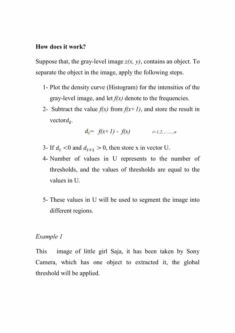
How does it work?
Suppose that, the gray-level image z(x, y), contains an object. To
separate the object in the image, apply the following steps.
1- Plot the density curve (Histogram) for the intensities of the
gray-level image, and let f(x) denote to the frequencies.
2- Subtract the value f(x) from f(x+1), and store the result in
vector .
= f(x+1) - f(x) i=1,2,……..,n
3- If 0 and 0, then store x in vector U.
4- Number of values in U represents to the number of
thresholds, and the values of thresholds are equal to the
values in U.
5- These values in U will be used to segment the image into
different regions.
Example 1
This image of little girl Saja, it has been taken by Sony
Camera, which has one object to extracted it, the global
threshold will be applied.

(a) (b) (c)
Figure 3.2 (a); Gray-level image of Saja picture;(b) Histogram of Saja image (c)Thresholded image
Figure 3.2(a), presents image of a little girl (Saja), which
converted to gray-level image by using MATLAB software.
Histogram of the pixels intensities of Saja image plotted in
Figure 3.2(b). The minima point in the histogram (valley point)
will be corresponded to value of thresholding in horizontal axis,
as in Figure 3.2 (b), thresholding is determined at T=(65.32).
Then all pixels which have intensity greater than this threshold
will set as foreground pixels, otherwise will be defined as
background, thresholded image shown in Figure 3.2 (c).

Local thresholding: Thresholding is called local or adaptive
thresholding when a different thresholds are used for different
regions in the image. Due to uneven illumination and other
factors, the background gray level and the contrast between the
objects and the background often vary within the image. In such
cases, global thresholding is unlikely to produce satisfactory
results, since a threshold that works well in one area of the
image might work poorly in other areas. To cope with this
variation, one can use an adaptive, or variable threshold. Liu
(2002)
When histogram of image contains many peaks and valleys, in
this case local thresholding will be used.
if <I (x,y) ≤
G(x, y) = B if I(x, y) ≤
if I (x, y) >
Where;
I(x, y): intensity of (any point) the image.
G(x,y) : the thresholded image.

: first local threshold.
: Second local threshold.
: first object class in the image.
: second object class in the image.
B: Background pixels.
Suppose that an image composed of light objects on a dark
background to extract the objects from the background local
thresholds have been applied to separate these objects from
background, then, any point (intensity value) (x, y) belonging to
first object class" ", if <I (x, y) ≤ , to the other object class
" ", if I (x,y) > ,and to the background if I(x, y) ≤ . See
Figure 3.3. This image taken from digital image processing
book.
Figure 3.3: Local thresholding
Object 1 Object 2Background

Since this research aims to detect one object in the image, then
the global thresholding will be used, this threshold will be
determined by using density curve or the histogram. This curve
may be unsmoothed, the smoothing curve is needed to find
optimum threshold.
Then the Scale-Space method will be presented as a method to
get optimum smoothing density curve, the next section explains
this method.
3.3 Scale-Space method
Scale is of vital importance in the analysis and understanding of
images. The classic example of a problem of scale. A forest can
only be recognized as such within a particular range of distance
(scales). If you are too close, the forest appears as a single
branch, piece of bark or collection of molecules. From a
distance of hundreds of kilometers the forest just becomes a
small part of the shape and texture of the landscape. The idea
that all information in an image is not contained at only one
scale is of crucial importance. It has been shown that to fully
analysis the structure of the image is necessary to relate
information from a number of different scales. Bradly (1995)
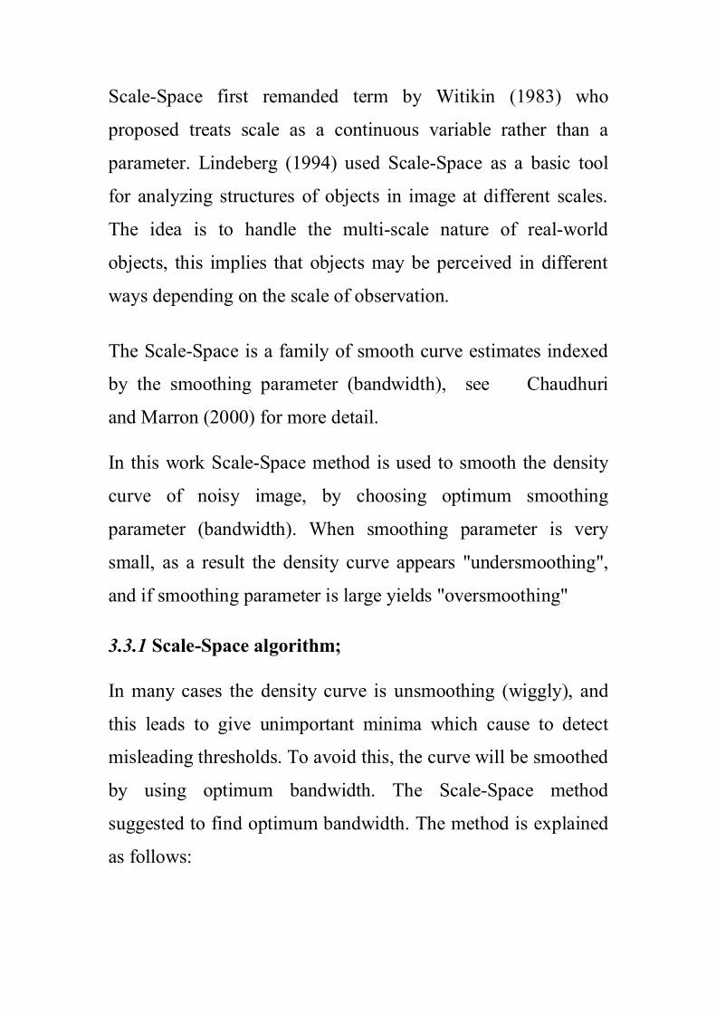
Scale-Space first remanded term by Witikin (1983) who
proposed treats scale as a continuous variable rather than a
parameter. Lindeberg (1994) used Scale-Space as a basic tool
for analyzing structures of objects in image at different scales.
The idea is to handle the multi-scale nature of real-world
objects, this implies that objects may be perceived in different
ways depending on the scale of observation.
The Scale-Space is a family of smooth curve estimates indexed
by the smoothing parameter (bandwidth), see Chaudhuri
and Marron (2000) for more detail.
In this work Scale-Space method is used to smooth the density
curve of noisy image, by choosing optimum smoothing
parameter (bandwidth). When smoothing parameter is very
small, as a result the density curve appears "undersmoothing",
and if smoothing parameter is large yields "oversmoothing"
3.3.1 Scale-Space algorithm;
In many cases the density curve is unsmoothing (wiggly), and
this leads to give unimportant minima which cause to detect
misleading thresholds. To avoid this, the curve will be smoothed
by using optimum bandwidth. The Scale-Space method
suggested to find optimum bandwidth. The method is explained
as follows:

1- Plot the density curve with initial bandwidth (automatic
bandwidth ), .
2- Set a limited sequence of bandwidth values with initial
bandwidth in the middle of the sequence B.
3- Plot the density curve with each value in the sequence, and
count numbers of minima (thresholds), which resulted
from each bandwidth, and store the result in vector .
4- From the sequence B, find the bandwidth values
corresponding to the values, which has most frequencies in
the vector , store the results in vector .
5- The optimum bandwidth is obtained as a median of values
in .
The optimum bandwidth is used to plot optimum density curve.
Then optimum threshold will be obtained from the optimum
density curve. (Elramly 2005)
Example 2
This example presents simulated histogram (Density curve),
with three levels of bandwidth, to faithful data from R software.
The first bandwidth very small, it is equal to 0.03 and it gives
undersmoothing curve, as shown in Figure 3.4(a). The curve in
Figure 3.4(b) smoothed by using a optimum bandwidth which
equal to 0.33 and this curve has two peaks and one valley.
Figure 3. 4(c) shows oversmoothing curve with large bandwidth
which equal to 2.

(a) (b) (c)
Figure3.4 : Simulated density curve with three levels of bandwidth;(a) under smoothing; (b) optimumsmoothing; (c) over smoothing
Example 3
This example shows image of a little girl (Saja) with different
scales, in Figure 3.5(a) Saja is completely appear when picture
will be taken at certain distance, but when this distance closer,
parts or some features of the body disappears as seen in Figure
3.5(b), and becomes shorter and shorter, more features will
disappear at each distance, cause change of scale which images
taken from. As seen in Figure 3.5 (c).
(a) (b) (c)
Figure 3.5: Saja picture with different scales; (a) large distance;(b) from close distance ;(c) shortestdistance.

3.4 Median filter method
Some images are affected by noise. The term noise is generally
taken to mean an undesired additive component of an image.
Filtering (smoothing) is an image processing operation that is
normally used to remove noise in an image or to enhance the
information already present for better appearance of certain
features, to facilitate subsequently more accurate image
analysis.
Several methods can be used to smooth images, such as, mean
filter, max-min filter, and median filter. In this work median
filter has been suggested to remove Salt-and-Pepper noise, in the
image under processing. Median filter is particularly effective in
the presence of impulse noise, also called Salt-and-Pepper noise
because of its appearance as white and black dots superimposed
on image.
Median filter not only smoothes noise in image regions, it also
tends to produce regions of constant or nearly constant intensity.
One of the main reasons for the popularity and wide-spread use
of median filter is its computational simplicity and good
performance in remove noise, see Pitas and venetsanopouls for
more detail (1992).
In order to perform median filtering at pixel in an image and its
neighborhood, first sort the value of the pixel and its
neighborhood, then determine median of this set, and replace the
value of pixel with median value, Gonzalez and Woods (2008).
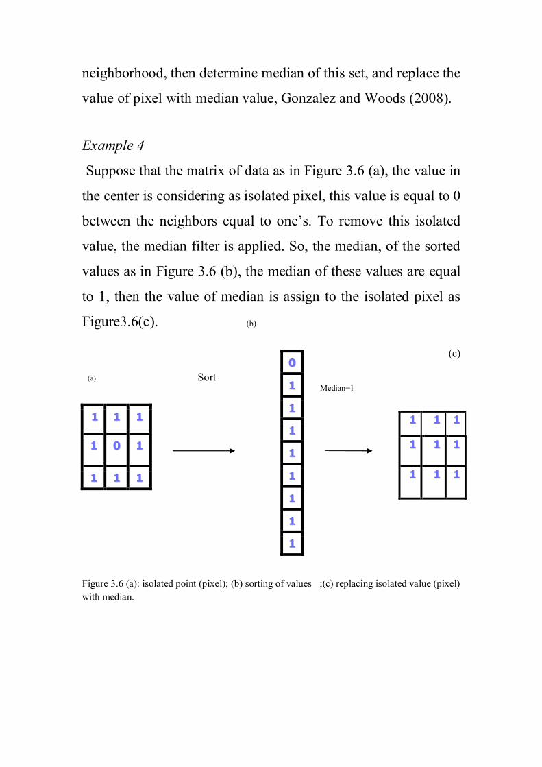
Example 4
Suppose that the matrix of data as in Figure 3.6 (a), the value in
the center is considering as isolated pixel, this value is equal to 0
between the neighbors equal to one’s. To remove this isolated
value, the median filter is applied. So, the median, of the sorted
values as in Figure 3.6 (b), the median of these values are equal
to 1, then the value of median is assign to the isolated pixel as
Figure3.6(c). (b)
(c)
(a) SortMedian=1
Figure 3.6 (a): isolated point (pixel); (b) sorting of values ;(c) replacing isolated value (pixel)with median.
00
11
11
11
11
11
11
11
11
111111
111111
111111
111111
110011
111111

3.5 Projection method
Projections transform points from n-space to m-space, where
m<n. Projections are a small set of transforms often used to
show profile of images. The concept of projection, normally
employed in Tomographic imaging (medical imaging), which is
the formation of an image of the slice of the body from a series
of projections through the body, also for displaying graphical
data.
Lehmann, et al. (2004) compared between two methods to
reconstructed image, which is Filter Back Projection (FBP) and
Algebraic Reconstruction Techniques (ART), both techniques
are tested by reconstructing a simulated object, showing that the
FBP technique yields images with better resolution and higher
contrast, thus resulting in more accurate information than
obtained by ART.
The goal of image reconstruction is to detect the object, by
using projection method, to reconstruct the image from
projection. Let an input image be defined by a discrete function
f (x, y). Then, a vertical projection ( ) of the function f at
point y is a summary of all pixel intensities in the column
of the input image. Similarly, a horizontal projection ( ) at
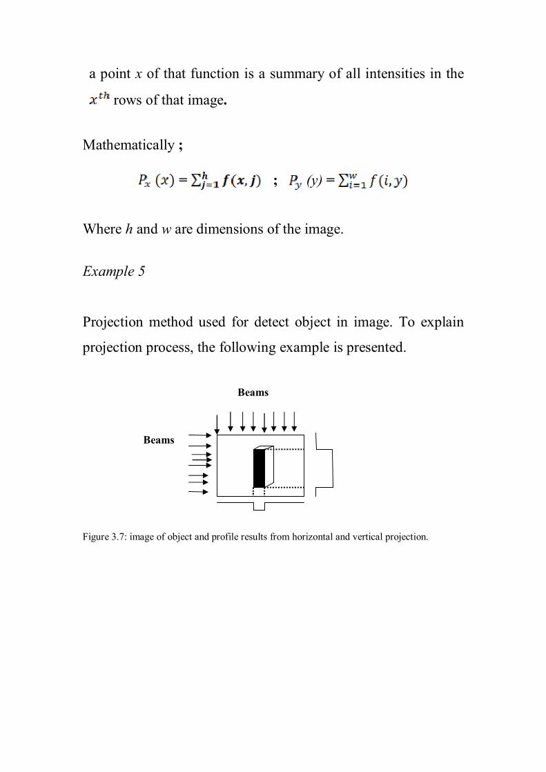
a point x of that function is a summary of all intensities in the
rows of that image.
Mathematically ;
= ; (y) =
Where h and w are dimensions of the image.
Example 5
Projection method used for detect object in image. To explain
projection process, the following example is presented.
Beams
B
Beams
Figure 3.7: image of object and profile results from horizontal and vertical projection.

In this example Figure (3.7) shows binary image with object ,
suppose that beam pass from left to right thought object
(horizontal projection), also beam pass from up to down thought
object that means (vertical projection), the horizontal projection
yields a profile of the object, which resulted from count the
pixels, and the profile is plotted in the left of the image. As same
the profile of the vertical projection is plotted in Figure (3.7).
From these two profiles the object can be reconstructed as
shown in Figure 3.8
Figure 3.8: reconstructed image

Chapter 4
Proposal algorithm
4.1 Introduction
This chapter proposes an algorithm that will be used to extract
object in the image.
The proposal algorithm has been made as a combination of
methods, the used methods in the algorithm are, segmentation
method, scale-space method, median filter method, and
projection method. These methods are used to specify features
of object and then reconstruct the object, according to the
location, size, and number of objects in the image.
4.2 Methods of the proposal algorithm
Before mention the steps of our algorithm, this section will give
a general view to understand the algorithm.
The first stage in the algorithm is the segmentation method
which is proposed to extract the object from the background.
Herein, the histogram-based thresholding method is applied to

segment the image into background and foreground. The
histogram will be presented as a density curve. This curve might
be oversmoothed or undersmoothed, then optimum bandwidth
(smoothing parameter) will be obtained and applied to the curve.
The Scale-Space method is used to get optimum bandwidth, this
bandwidth will be used to find optimum smoothing curve, and
then obtained optimum threshold value, which use to plot
thresholded image.
The isolated pixels (Salt-and-Pepper noise), may be appeared in
the thresholded image, then median filter method is suggested to
remove this kind of noise.
Now, the binary image is obtained, to identify location, size and
number of the objects in image the projection method will be
applied.
The following diagram explains the stages of the suggestedalgorithm.

Input noisy image
Output
Figure 4.1: Diagram of the proposal algorithm
Segmentationmethod
Scale-Spacemethod
Median filtermethod
Projection
Method
Location, size and numberof objects determination
4.3 Algorithm
The aim of the algorithm is to detect a geometrical object ,which
has a square shape in the image. The algorithm can be
summarized in the following steps:
1- Plot the histogram (Density curve) of the image, to find the
threshold, due to noise or different colours in the image.
The density curve will be unsmoothed. Then to smooth the
curve, the optimum bandwidth (smoothing parameter)
should be obtained.
2- Use Scale-Space method to find optimum bandwidth,
which use to obtain optimum threshold,
see SubSection (3.3.1).
3- Segment the image into background and foreground by
using optimum obtained threshold, then plot binary
image, which may be containing some Salt-and-Pepper
noise
4- Apply median filter to remove unwanted pixels (Salt-
and-Pepper noise) may appear in the obtained binary
image.

5- Use projection method, to obtain the horizontal and
vertical profiles, from the binary image.
6- Determine the location, size and number of objects, by
using the change points in the horizontal and the
vertical profiles.
7- Use the obtained points in the previous step to reconstruct
the object.
The algorithm will be explained and evaluated by using
simulated data in the next chapter, if it yields good results
then the algorithm will be implemented to real data.

Chapter 5 Applications
5.1 Introduction
As mentioned before, this chapter presents two kinds of
applications. The first kind is application to synthetic data,
which has been used to evaluate the proposed algorithm. If the
algorithm to simulated data works well, then it will be applied to
real data.
Next section introduce model, which can be used to create a
simulated data and shown the three parameters (number, size
and location of objects).
5.2 Simulated Data
This section describes an image consists of a square shape as an
object. The object is defined by three parameters, which are
number, location and size.
Suppose that the location of the square object is define by (x, y),
which are location coordinates. The size of the object is

determining by and , is the length(height), and
indicates width of the object, while number of the objects has
been termed by N.
Mathematically;
N~pois ( “N=number of objects”
X~pois( )
Y ~ pois( )
Where; X and Y are location coordinates
~ pois( )
~ pois( )
Where; =length, =width
Assume that, A is a matrix of zeros of size n × m
Where;
n ~ pois( )
m ~ pois ( )
Note that, , , , , are supposed to be
chosen with restriction . where 0< λ < ∞
Then the elements from the row X till (X+ ) , and fromthe column y till (y+ ) , are setting to be ones.
The matrix A will give binary image with black object andwhite background. This matrix will be contaminated byadding Gaussian noise, the resulted matrix is termed as f,where; = aij +

i=1, 2,…, m and j=1,2,…, n
Where e is distributed random normal with mean M andvariance .
5.3 Application to simulated data.
In this section, the image has been simulated with onegeometrical object (square shape), the resolution is (40000)pixels, with dimensions 200 by 200, and displays inFigure (5.1). That is, n=200 and m=200.
· N indicates to number of objects in the image, where
this parameter generated from Poisson distribution in
this application N=1.
· Location coordinates (x, y) are generated from
Poisson distribution with and equal to 100 ,
( =100 and =100).
· Size of object defined by height (length) and width of
the object ( , ) respectively, which are followed
Poisson distribution, with =50, =50 .

Figure 5.1: Simulated data
The simulated data, in Figure 5.1, is displayed as binary
image in Figure 5.2. The foreground represents the object
(square shape) while the rest of image is background with
intensities equal to 1 and 0 respectively.
y
x,

Figure5.2: Binary image of simulated data
The binary image is contaminated by adding Gaussian noise
with mean equal to zero and standard deviation equal to 0.2,
the noisy image is shown in Figure 5.3.
Figure5.3: Noisy image of simulated data
According to proposed algorithm, the image will be segmented
into foreground and background. Then, thresholding approach is
applied, to obtain the value of threshold, the noisy image density
curve is plotted. Some of unimportant minima are appears, as in
Figure (5.4). This leads to detect some misleading thresholds
(local thresholds).

Figure5.4: Density curve of noisy image
To remove un-wanted minima, the algorithm suggests to smooth
the curve of noisy image. This step is done by looking for
optimum bandwidth (smoothing parameter), which is used to
plot optimum density curve. To do so Scale-Space method most
be applied. Figure (5.5) displays the diagram of the Scale-Space,
it shows one tail that lasting longest the other. This means that
the data has one threshold, and the optimum bandwidth is
corresponding to median of the values of the longest tail in the
Scale-Space diagram.

Bandwidths
Figure 5.5: Scale-Space diagram for data
The optimum bandwidth is found to be = 0.12,( at vertical solid
line in diagram), this value is used to smooth noisy image curve
as in Figure (5.6), then the optimum value of threshold equal to
T= 0.7, is obtained.
Thre
s hol
ds

T=0.7
Figure 5.6; Optimum smoothing density curve
The optimum threshold is used to segment the noisy image, but
some isolated pixels (Salt & Pepper noise) are appears,
Figure 5.7, displays the image with isolated pixels.
Figure 5.7: Binary image with Salt and Pepper noise
The median filter is proposed to remove this noise. Where
median filter method is used as a third stage in proposal
algorithm, and the result is displayed in Figure 5.8.

Figure 5.8: Filtered image
The next step in proposal algorithm is a projection method
(step 5 in section 4.3). This method is used to detect the
main parameters to define the object. In this method, the
values in each column are summed, and saved in vector
(vertical projection). The result of the vertical projection is
plotted in Figure 5.9.

Figure 5.9: Vertical projection plot
This Figure shows that there is one object in the image,the values in the vector are:
=( 0 0 0 0 0 0 0 0 0 0 0 0 0 0 0 0 0 0 0 0
0 0 0 0 0 0 0 0 0 0 0 0 0 0 0 0 0 0 0 0
0 0 0 0 0 0 0 0 0 0 0 0 0 0 0 0 0 0 0 0
0 0 0 0 0 0 0 0 0 0 0 0 0 0 0 0 0 0 0 0
0 0 0 0 0 0 0 0 0 0 0 40 43 43 43 43 43 43
43 43 43 43 43 43 43 43 43 43 43 43 43 43 43 43
43 43 43 43 43 43 43 43 43 43 43 43 43 43 43 43
43 43 43 41 41 0 0 0 0 0 0 0 0 0 0 0 0 0 0
0 0 0 0 0 0 0 0 0 0 0 0 0 0 0 0 0 0 0 0
0 0 0 0 0 0 0 0 0 0 0 0 0 0 0 0 0 0 0 0
0 0 0 0 0 0 0 0 0 0 0 )
The positions of non-zeros values in vector are takenout in a new vector ( c ), and they are;
Pc= ( 92 93 94 95 96 97 98 99 100 101 102 103 104
105 106 107 108 109 110 111 112 113 114 115 116
117 118 119 120 121 122 123 124 125 126 127 128
129 130 131 132 133 134 135 )
This vector has continuous values, which means the image
contains one object, the first value 92, and the last value
135, in the vector Pc are determined the edges of the
object horizontally. While the difference between those
values gives the horizontal size of the object.
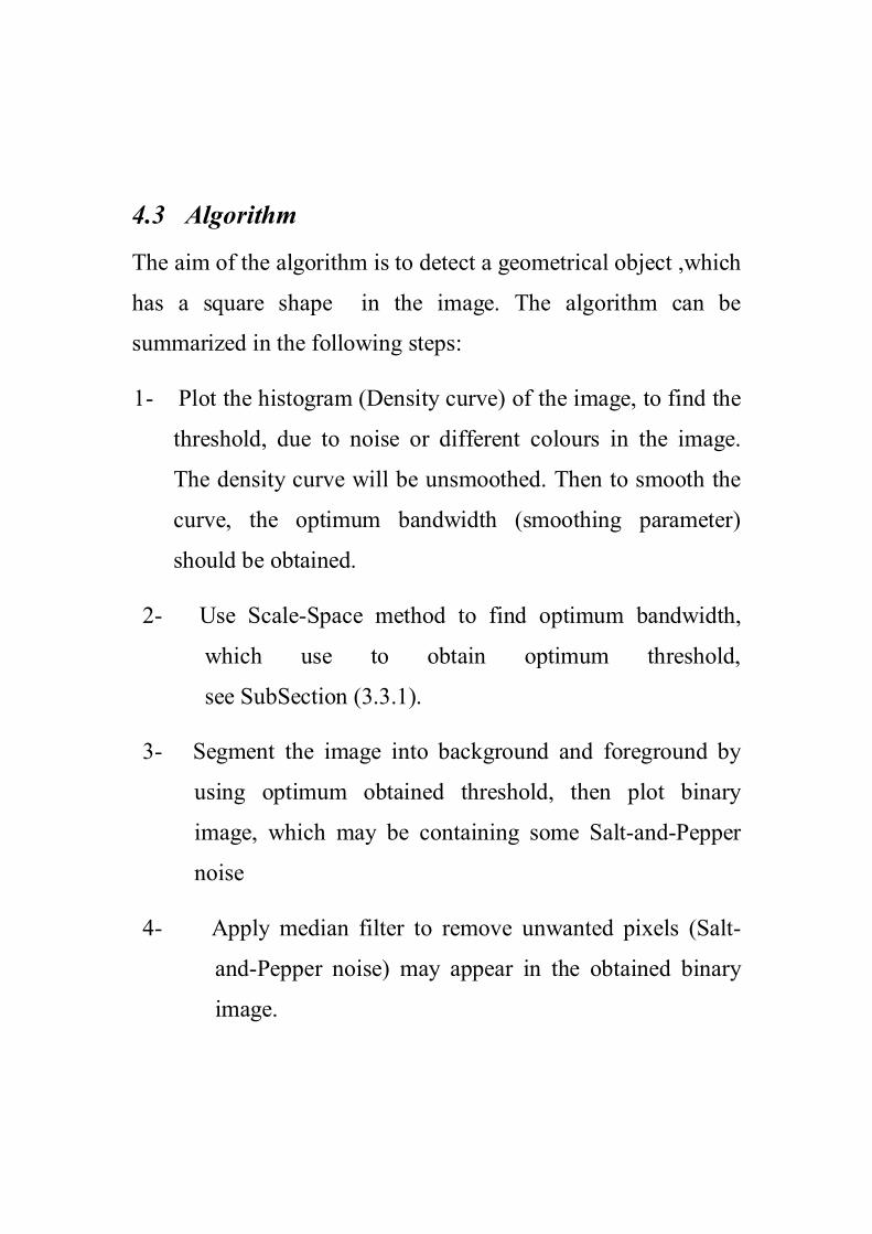
The same procedure is conducted on rows (Horizontal
projection), and the results are plotted in Figure (5.10).
This Figure confirms that the number of object in image is
one.
Figure 5.10: Horizontal Projection

The values, which are results from this step, are stored in
vector , where;
= ( 0 0 0 0 0 0 0 0 0 0 0 0 0 0 0 0 0 0 0 0 0 0 0
0 0 0 0 0 0 0 0 0 0 0 0 0 0 0 0 0 0 0 0 0 0 0 0
0 0 0 0 0 0 0 0 0 0 0 0 0 0 0 0 0 0 0 0 0 0 0 0
0 0 0 0 0 0 0 0 0 44 44 44 44 44 44 44 44 44 44 44 44
43 43 44 44 44 44 44 44 44 44 42 42 44 44 44 44 44 44 44
44 44 44 44 44 44 44 44 44 44 44 43 0 0 0 0 0 0 0 0 0
0 0 0 0 0 0 0 0 0 0 0 0 0 0 0 0 0 0 0 0 0 0 0 0
0 0 0 0 0 0 0 0 0 0 0 0 0 0 0 0 0 0 0 0 0 0 0 0
0 0 0 0 0 0 0 0 0 0 0 0 0 0 0 0 0 0 0 0 )
The positions, of the non-zeros values in are;
= ( 81 82 83 84 85 86 87 88 89 90 91 92 93 94 95
96 97 98 99 100 101 102 103 104 105 106 107 108 109
110 111 112 113 114 115 116 117 118 119 120 121 122
123)
Since the values in this vector without any gap, then the object
in the image is one, and this result is confirmed by the previous
figure.
To reconstruct the square shape, the four points in four corners
are needed. Then these points are formulated by taking the first

Point in vector Pc corresponding to the first and the last points
in , and the last point in the with the first and the last
points in . This step yields;
(92, 81),(92, 123),(135, 81),(135, 123)
These coordinates are used to reconstruct the object as inFigure(5.11).
Figure 5.11: Reconstructed dataset
y
x
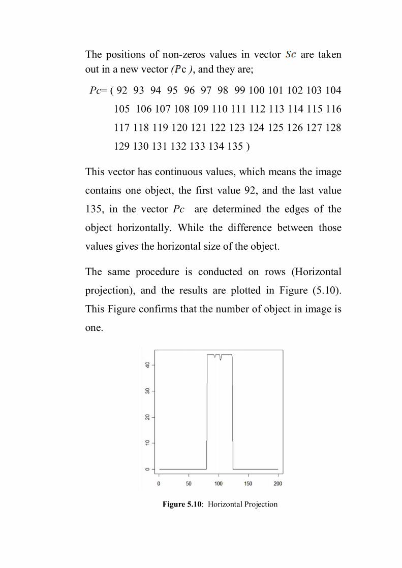
The vertical size is calculated by subtract the last value in
from the first point in that is
- = 123 - 81 = 42
Also horizontal size
- =135- 92= 43
The algorithm yields good results, to detect the three parameters
which are used to reconstruct the object.
These parameters are;
Location coordinates (x, y), which are
(92, 81),(92, 123),(135, 81),(135, 123)
And the size of the object ( , ) equal to (42, 43), and N that
indicates to number of the objects in the image, and it equal to 1

5.4 Application to real data
In this example the algorithm will be applied to real data, which
represents remotely sensed image. The image has been taken
from Google Earth site (www.googleEarth.com), in the internet,
this image is displayed in Figure 5.12. The image is for a farm
in Tripoli-Libya, it consists of black square object.
Figure 5.12: Image to farm in Tripoli
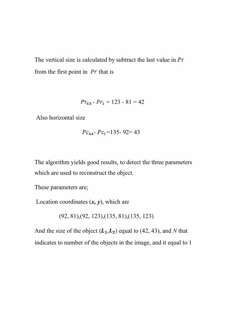
The image has been converted into Gray-level by usingMATLAB software (version.7.6), and shown in Figure 5.13.
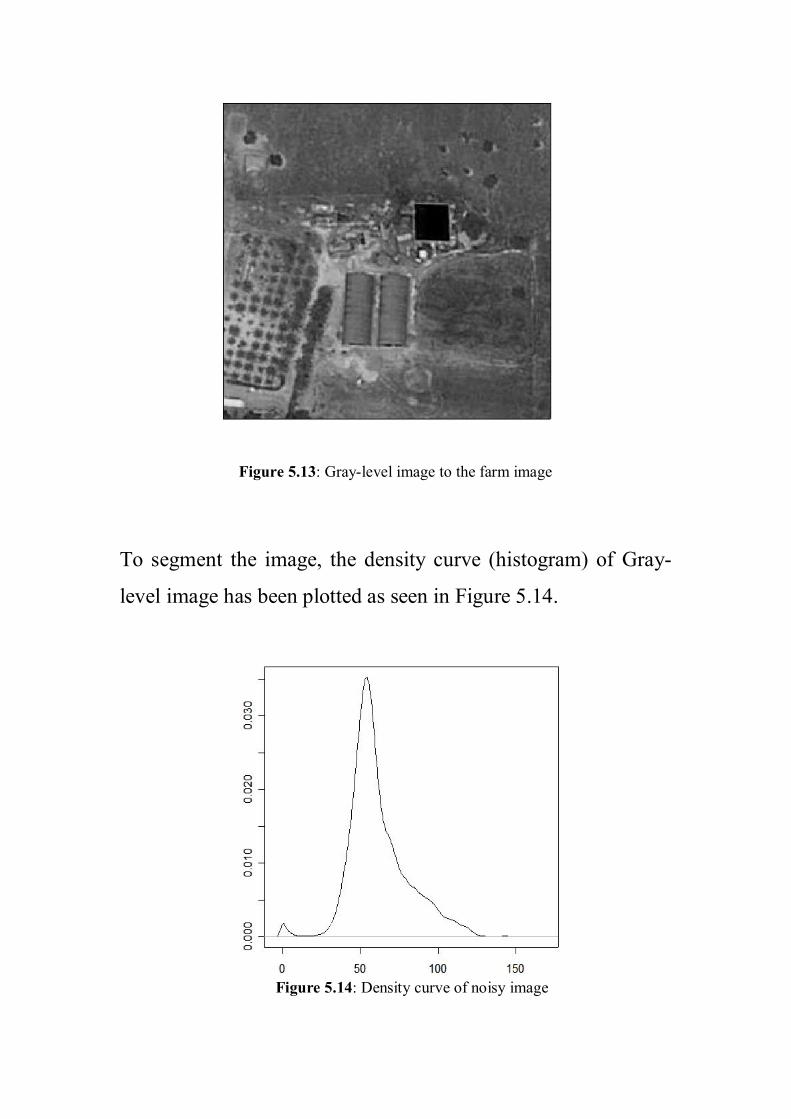
Figure 5.13: Gray-level image to the farm image
To segment the image, the density curve (histogram) of Gray-
level image has been plotted as seen in Figure 5.14.
Figure 5.14: Density curve of noisy image

Looking at Figure 5.14 illustrated, there is a single threshold,
but some local minima might lead to detect extra incorrect
thresholds. To get optimum threshold the curve should be
smoothed, then the optimum bandwidth is needed. To do so, the
Scale-Space method is used. Figure 5.15, shows graphic form of
Scale-Space method.
bandwidths
Figure 5.15: Scale-Space diagram for the real data.
The optimum bandwidth (smoothing parameter) equal to 7.30,
which obtained by Scale-Space method, is used to plot optimum
histogram as in Figure 5.16.
Thre
shol
des

Figure 5.16: Smoothed density curve for the real data.
Then the optimum threshold is obtained from the optimum
histogram and it found to be equal to 13.81, this is shown as
vertical line in Figure 5.16.
Figure 5.17: Thresholded image
The optimum threshold is used to segment the image into object
and background as seen in Figure 5.17. The thresholded image
has had some isolated pixels as noise. The median filter has
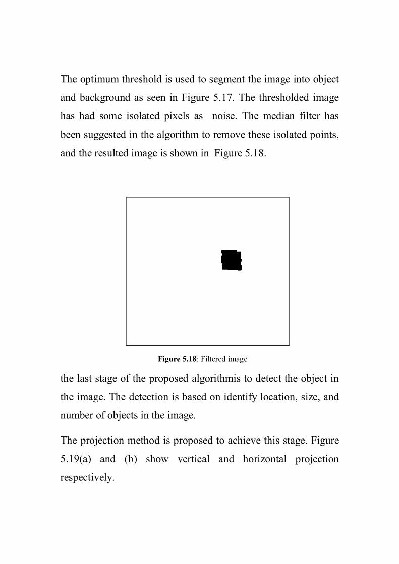
been suggested in the algorithm to remove these isolated points,
and the resulted image is shown in Figure 5.18.
Figure 5.18: Filtered image
the last stage of the proposed algorithmis to detect the object in
the image. The detection is based on identify location, size, and
number of objects in the image.
The projection method is proposed to achieve this stage. Figure
5.19(a) and (b) show vertical and horizontal projection
respectively.

(a)
(b)
Figure 5.19: (a) Vertical projection (b) Horizontal projection
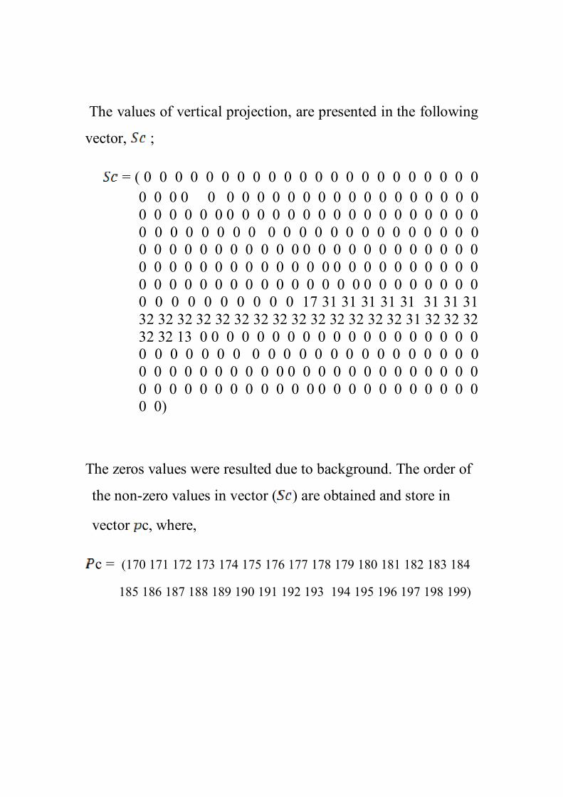
The values of vertical projection, are presented in the following
vector, ;
= ( 0 0 0 0 0 0 0 0 0 0 0 0 0 0 0 0 0 0 0 0 0 00 0 0 0 0 0 0 0 0 0 0 0 0 0 0 0 0 0 0 0 0 00 0 0 0 0 0 0 0 0 0 0 0 0 0 0 0 0 0 0 0 0 0 00 0 0 0 0 0 0 0 0 0 0 0 0 0 0 0 0 0 0 0 0 00 0 0 0 0 0 0 0 0 0 0 0 0 0 0 0 0 0 0 0 0 0 00 0 0 0 0 0 0 0 0 0 0 0 0 0 0 0 0 0 0 0 0 0 00 0 0 0 0 0 0 0 0 0 0 0 0 0 0 0 0 0 0 0 0 0 00 0 0 0 0 0 0 0 0 0 17 31 31 31 31 31 31 31 3132 32 32 32 32 32 32 32 32 32 32 32 32 32 31 32 32 3232 32 13 0 0 0 0 0 0 0 0 0 0 0 0 0 0 0 0 0 0 00 0 0 0 0 0 0 0 0 0 0 0 0 0 0 0 0 0 0 0 0 00 0 0 0 0 0 0 0 0 0 0 0 0 0 0 0 0 0 0 0 0 0 00 0 0 0 0 0 0 0 0 0 0 0 0 0 0 0 0 0 0 0 0 0 00 0)
The zeros values were resulted due to background. The order of
the non-zero values in vector ( ) are obtained and store in
vector c, where,
c = (170 171 172 173 174 175 176 177 178 179 180 181 182 183 184
185 186 187 188 189 190 191 192 193 194 195 196 197 198 199)

The vector of horizontal projection values ( ) and their
positions ( ) are :
= ( 0 0 0 0 0 0 0 0 0 0 0 0 0 0 0 0 0 0 0 0 0 00 0 0 0 0 0 0 0 0 0 0 0 0 0 0 0 0 0 0 0 0 0 00 0 0 0 0 0 0 0 0 0 0 0 0 0 0 0 0 0 0 0 0 0 00 0 0 0 0 0 0 0 0 0 0 0 0 0 0 0 0 0 0 0 0 0 00 0 0 0 0 0 0 0 0 0 0 0 0 0 0 0 0 0 0 0 0 0 00 0 0 0 0 0 0 0 0 0 0 0 0 0 0 0 0 0 0 0 0 0 00 0 0 0 0 0 0 0 0 0 0 0 0 0 0 0 0 0 0 0 0 0 00 0 5 21 29 29 29 29 29 29 29 28 28 28 29 29 29 30 3030 30 30 29 29 29 29 29 28 28 28 28 29 29 29 23 0 0 00 0 0 0 0 0 0 0 0 0 0 0 0 0 0 0 0 0 0 0 0 0 00 0 0 0 0 0 0 0 0 0 0 0 0 0 0 0 0 0 0 0 0 0 00 0 0 0 0 0 0 0 0 0 0 0 0 0 0 0 0 0 0 0 0 0 0 00 0 0 0 0 0 0 0 0 0 0 0 0 0 0 0 0 0 0 0)
= (163 164 165 166 167 168 169 170 171 172 173 174 175 176 177
178 179 180 181 182 183 184 185 186 187 188 189 190 191 192 193 194
195)
The values, in the vectors c and , are consecutivenumbers, and this means the image contains of one object.
The first value in vector c determines the first pixel in theobject respect to vertical coordinate, while the last value in thevector c is corresponded to the last pixel in the object in thevertical coordinate.
This will be same in case of horizontal projection, to gethorizontal coordinates, these points will be used to determine
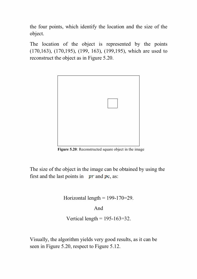
the four points, which identify the location and the size of theobject.
The location of the object is represented by the points(170,163), (170,195), (199, 163), (199,195), which are used toreconstruct the object as in Figure 5.20.
Figure 5.20: Reconstructed square object in the image
The size of the object in the image can be obtained by using thefirst and the last points in and c, as:
Horizontal length = 199-170=29.
And
Vertical length = 195-163=32.
Visually, the algorithm yields very good results, as it can beseen in Figure 5.20, respect to Figure 5.12.

Chapter 6
Summery and Conclusions
6.1 Summary
This study presents an algorithm to identify the geometrical
object in the images. To identify the object from the image,
three main characteristics should be obtained; number, size,
and location of that object. This algorithm contains of number
of approaches; segmentation method which is used to extract
the foreground from background by histogram-based
thresholding technique, Scale-Space method is adopted to find
the optimum bandwidth that is used to obtain optimum
smoothing curve, and then obtained optimum threshold value,
which use to segment thresholded image, median filter has
been applied to remove the isolated pixels (Salt and Pepper
noise) may be arise in the thresholded image, the previous
methods used to get binary image, to detect the main
characters of square object in the image, projection method was
applied.
6.2 ConclusionsThe proposed algorithm, in this project, has been evaluated by
using a synthetic data and achieved good results. This achieved
encouraged to apply the algorithm to real data, the presented in
example with image has square shape of object in this thesis. In
case of real data, algorithm yields well result. The algorithm
provided good results and achieved the aims of this research when
the image contain one object, but such good results were not be
possible when the objects in image are overlapped.
6.3 Future work
· In this project, number of objects was supposed to be one,
in future this character might be unknown and it simulated
from discrete distribution.
· Also, if the image contains more than object, the algorithm
should be modified to handle case of overlapping between
the objects.
· The aim of this study was detected geometrical object
according to its main characteristics; location, size and

number. This objective can be developed to identify non-
geometric objects, such as; handwriting, fingerprint, and
etc.
• Try to determine the true shape of the object.
• The image that was analyzed was converted to gray scale,
in the future try to analysis the multi-color image.

REFERENCES
1. Balazs, P. (2007), Reconstructing some Hv-convex Binary Images
from Three or Four Projections, proceedings of the 5th International
symposium on image and signal processing and analysis(ISPA07),
136-140.
2. Besag, J. (1986), on the statistical Analysis of Dirty Pictures (with
discussion), Journal of the Royal statistical society B 48, 259-302.
3. Chaudhuri, P. and Marron, J. S. (2000), Scale-Space View of
Curve Estimation, The Annals of statistics, 28, 408-428.
4. Chan, R. H. and Nikolova, M. (2005), Salt-and-Pepper Noise
Removal by Median-Type Noise Detectors and Detail-Preserving
Regularization. IEEE Transactions on image processing, 14, 1479-
1485.
5. Elramly, F .M. (2005), Geometrical Modeling and Identification of
Structure in Image Data, unpublished p.h D thesis, Leeds, UK.
6. Eng, H.-L. and Ma, K.-K. , (2001), Noise Adaptive Soft-Switching
Median Filter. IEEE Transactions on Image processing , 10. 242-
251.
7. Glasbey, C. A. and Horgan, G. W.(1995), Image Analysis for the
Biological Sciences, John Wiley and Sons, Hall, Chichester.

8. Geman, S. Geman, D .(1984) , Stochastic Relaxation Gibbs
Distribution, and the Bayesian restoration of images. IEEE Trans.
Pattern Anal. Machine Intell.6, 721-741.
9. Gonzalez, R. C. and Woods, R. E. (2008), Digital Image Processing.
3rd , Pearson Prentice Hall, New Jersey.
10. Goudail, F. and Refregier, P. (2004). Statistical image processing
Techniues for Noisy Images. Spring, New York.
11. Huang, L.-K. and Wang, M.-J. J. (1995), Image Thresholding by
Minimizing the Measures of Fuzziness, Pattern Recog., 28, 41-51.
12.
13. Jones, M. C. and Sheather, (1996), A Brief Survey of Bandwidth
Selection for Density Estimation, Journal of the American Statistical
Association, 91, No. 433.
14. Khamitkar, S. D., Kalyankar, N. V. and Al-amri, S. S. (2010),
Image Segmentation by using Threshold Techniques, journal of
computing, 2, ISSUE5, 83 -86.
15. Lehmann, E. H, Bucherl, T, Megahid, R. M, and Ali, A. M,
(2004), Image Reconstruction Techniques using Projection data
from Transmission Method, Annals of Nuclear Energy, 31, 1415-
1428.
16. Lindeberg, T. (1994), Scale-Space Theory: A basic Tool for
Analyzing Structures at Different Scales, Statistics and Images, 21,
225-270.
17. Liu, F. (2002), Adaptive Thresholding Based on Variational
Background, Electronics Letters, 38, 1017-1018.
18. Lukac, R. (2003), Adaptive vector median filtering. Pattern
Recognition Letters. In Elsevier. 24, 1889–1899.
19. Mardia, K. V. and Dryden, I. L. (1998), Statistical Shape Analysis,
John Wiley and sons, Hall, Chichester

20. Otsu, N. (1979), a threshold Selection Method from Gray- Level
Histogram, IEEE Transactions. On Systems, MAN, and Cybernetics
9, 62-66.
21. Pitas, I. and Venetsanopoulos, N. A. (1992), Order Statistic in
Digital Image Processing, IEEE Transactions on image processing,
80, 1893-1921.
22. Qiang, W. U. and Castleman, K. R. (2008), Microscope
Image Processing, Elsevier, California.
23. Tukey, J.K.(1974), Nonlinear ( nonsuperposable ) methods for
smoothing data, in Proc. Congr Rec. EASCOM, P. 637
24. Tobias, O.J. and Seara, R. (2002), Image Segmentation by
Histogram Thresholding Using Fuzzy Sets, IEEE Transactions on
Image Processing,11, 1457-1465.
25. Witkin, A. P. (1983), Scale-Space filtering. In Proc. Eight
International Joint Conference on Artificial Intelligence, Karlsruhe,
Germany, 1019-1022.
26. Zhang, T. , Lu, H. and Yan, L. (2000), Threshold Selection using
Partial Structural Similarity, International Journal of Digital Content
Technology and its Applications. 5, 397-407.

معة بنغازيجاكلیة العلوم
الإحصاءقسم
في الصورةھندسيلشكد خوارزمیة لتحدی
إعداد
دعاء ونیس إدریس احمد
إشراف
فتحي محمد الرملي . د
ات الحصول علي رسالة التخصص العالي لغرض استكمال متطلبالإحصاءالماجستیر في قسم
لیبیا-بنغازي
2012

الخلاصة
بطرق الصورتنتج،لمعلومات في كثیر من مجالات البحث العلميلمھمالصور مصدرتعتبر
ت و الرادارات والمجھر الالكتروني وغیرھا من الكامیراعلي سبیل المثال مختلفة منھا
یشیران إلي )(x ,yمكن تعریف الصورة الرقمیة علي إنھا دالة في بعدین ھما ی. الأجھزة
.تسمى كثافة الصورة عند تلك النقطةتلك النقطةإحداثیات الموقع وقیمھ الدالة عند
تحتوي علي مجموعة من خوارزمیة وضعلتحدید الشكل الھندسي في الصورة نحتاج إلي
:طرق ھيه الذلك الھدف وھذسالیب لانجاز الأ
ثم طریقة فراغ ،عن الخلفیة) الشكل الھندسي (جھة طریقة الفصل ونحتاج إلیھا لفصل الوا
.المقیاس لتنعیم منحنى كثافة الصورة ثم طریقة مرشح الوسیط لتخلص من النقاط المعزولة
الأولى من الخوارزمیة و حصولنا علي الصورة الثنائیة باللونین الأسود المراحلبعد تنفیذ
نكون قد توصلنا إلي مرحلة ، وتكون الصورة خالیة من التشویش ، جسم والأبیض للخلفیة لل
فاننا سوف ،ثم اعتمادا علي طریقة الإسقاط . التعرف أو تمییز الشكل الموجود داخل الصورة
.نحدد عدد و مواقع وحجم الأجسام
بالتالي تم تطبیقھا ، دهأعطت نتائج جی، عند تطبیق ھذه الخوارزمیة علي البیانات الاصطناعیة
علي البیانات الحقیقیة وحققت ما نھدف إلیھ في ھذا البحث وھو التعرف علي شكل ھندسي في
.صورة الرقمیة

Appendix
R-code for the proposed algorithm
z=matrix(0,200,200)
x=rpois(1,100)
y=rpois(1,100)
l1=rpois(1,50)
l2=rpois(1,50)
z[x:(x+l1),y:(y+l2)]=1
image(z,col=gray(64:0/64),axes=F);box()
##########add Gaussian noise to image###############
z1=z+rnorm(200*200,0,0.2)
image(z1,col=gray(64:0/64),axes=F);box()
##################Scale-Space Method ############
a= density((z1))
ha=a$bw
d=80
b= seq((ha*0.1),(ha*10),length=d)

ydn=0
u=matrix(0,d,510)
for(i in 1:length(b)){
a1=density((z1),b[i])
yd=a1$y
for(j in 1:(length(yd)-1)){
ydn[j]=yd[j+1]-yd[j] }
xt=0
for(k in 1:(length(yd)-2)){
if(ydn[k]<0 & ydn[k+1]>0){
xt[k]=a1$x[k+1]}else{
xt[k]=0} }
u[i,]=xt}
yu=NULL
for(i in 1:d){
yu=c(yu,which(u[i,]!=0))
}
xb= NULL
for(i in 1:d){
xb=c(xb,rep(b[i],length(which(u[i,]!=0)))) }
plot(xb,yu)
r=NULL
for( i in 1: d){
r = c(r,length(which(u[i,]!=0)))
}
rr=unique(r)
B=0
for(i in 1:length(r)){
B[i]=length(which(rr[i]==r))
}
BB=rr[which.max(B)]
q=which(r==BB)
########## Optimum Bandwidth (bwo) #####
bwo=median(b[q])
w=density(z1,bwo)
yz1=w$y
m=0
for(i in 1:(length(yz1))-1){
m[i]=yz1[i+1]-yz1[i] }
d=NULL
for( i in 1:(length(m)-1)){
if(m[i]<0 && m[i+1]>0){
d=rbind(d,i)
}}
plot(w)
abline(v=w$x[d])
T=w$x[d]
##########Optimum Thresholdng #####
zt=matrix(0,nrow(z1),ncol(z1))
for(i in 1:nrow(z1)){
for(j in 1:ncol(z1)){
if(z1[i,j]>T){
zt[i,j]=1}else{
zt[i,j]=0}
}}
image(zt,col=gray(64:0/64),axes=F);box()
########## median filter procedure ############
## It use for remove salt and paper noise #####
neigh = function(x,i){
neigh = c(i-1,i+1,i-ncol(x),i+ncol(x),
i-ncol(x)-1,i+ncol(x)-1,i-ncol(x)+1,i+ncol(x)+1)
neigh = neigh[neigh>0]
neigh = neigh[neigh<=length(x)]
return(neigh)}
# Median smoothing filter - good for isolated outliers
medianfilter=function(x){
nc = ncol(x); nr = nrow(x)
output = matrix(0,nrow=nr ,ncol=nc)
for (i in 1:nc){
for (j in 1:nr){
neigh = x[i,j]
if(i>1 )neigh = c(neigh,x[i-1,j])
if(i<nc)neigh = c(neigh,x[i+1,j])
if(j>1 )neigh = c(neigh,x[i,j-1])
if(j<nr)neigh = c(neigh,x[i,j+1])
output[i,j] = median(neigh)
}}
return(output)
}
zm=medianfilter(zt)
####### binary image ###########
image(zm,col=gray(64:0/64),axes=F);box()
###### projection method ##########
dim(zm)
nr=nrow(zm)
nc=ncol(zm)
x11()
sc=0
for ( i in 1:nr){
sc[i]=sum(zm[i,])
}

plot(sc,type="l")
pc=which(sc!=0)
x11()
sr=0
for(i in 1:nc){
sr[i]=sum(zm[,i])
}
plot(sr,type="l")
pr=which(sr!=0)
######### reconstructed data #########
x1=c(pc[1],pc[1],pc[length(pc)],pc[length(pc)],pc[1])
x2=c(pr[1],pr[length(pr)],pr[length(pr)],pr[1],pr[1])
plot(x1,x2,type="l",xlim=c(0,200),ylim=c(0,200))