This article was downloaded by: [128.173.125.76] On: 21 February 2014, At: 12:06Publisher: Institute for Operations Research and the Management Sciences (INFORMS)INFORMS is located in Maryland, USA

INFORMS Journal on Computing

Publication details, including instructions for authors and subscription information:http://pubsonline.informs.org

An Algorithm for Fast Generation of Bivariate PoissonRandom VectorsKaeyoung Shin, Raghu Pasupathy,

To cite this article:Kaeyoung Shin, Raghu Pasupathy, (2010) An Algorithm for Fast Generation of Bivariate Poisson Random Vectors. INFORMSJournal on Computing 22(1):81-92. http://dx.doi.org/10.1287/ijoc.1090.0332

Full terms and conditions of use: http://pubsonline.informs.org/page/terms-and-conditions

This article may be used only for the purposes of research, teaching, and/or private study. Commercial useor systematic downloading (by robots or other automatic processes) is prohibited without explicit Publisherapproval. For more information, contact permissions@informs.org.

The Publisher does not warrant or guarantee the article’s accuracy, completeness, merchantability, fitnessfor a particular purpose, or non-infringement. Descriptions of, or references to, products or publications, orinclusion of an advertisement in this article, neither constitutes nor implies a guarantee, endorsement, orsupport of claims made of that product, publication, or service.

Copyright © 2010, INFORMS

Please scroll down for article—it is on subsequent pages

INFORMS is the largest professional society in the world for professionals in the fields of operations research, managementscience, and analytics.For more information on INFORMS, its publications, membership, or meetings visit http://www.informs.org

INFORMS Journal on ComputingVol. 22, No. 1, Winter 2010, pp. 81–92issn 1091-9856 �eissn 1526-5528 �10 �2201 �0081

informs ®

doi 10.1287/ijoc.1090.0332©2010 INFORMS

An Algorithm for Fast Generation ofBivariate Poisson Random Vectors

Kaeyoung Shin, Raghu PasupathyGrado Department of Industrial and Systems Engineering, Virginia Polytechnic Institute and State University,

Blacksburg, Virginia 24061 {pman93@vt.edu, pasupath@vt.edu}

We present the “trivariate reduction extension” (TREx)—an exact algorithm for the fast generation of bivari-ate Poisson random vectors. Like the normal-to-anything (NORTA) procedure, TREx has two phases:

a preprocessing phase when the required algorithm parameters are identified, and a generation phase whenthe parameters identified during the preprocessing phase are used to generate the desired Poisson vector. Weprove that the proposed algorithm covers the entire range of theoretically feasible correlations, and we pro-vide efficient-computation directives and rigorous bounds for truncation error control. We demonstrate throughextensive numerical tests that TREx, being a specialized algorithm for Poisson vectors, has a preprocessing phasethat is uniformly a hundred to a thousand times faster than a fast implementation of NORTA. The generationphases of TREx and NORTA are comparable in speed, with that of TREx being marginally faster. All code ispublicly available.

Key words : statistics; simulation; random variable generation; multivariate distribution; correlationHistory : Accepted by Marvin Nakayama, Area Editor for Simulation; received March 2008; revisedSeptember 2008, March 2009; accepted March 2009. Published online in Articles in Advance August 18, 2009.

1. IntroductionThe problem of generating random variables from aPoisson distribution with given parameter � > 0 iswell studied, and there currently exist very fast gen-eral procedures for implementation on a digital com-puter. See Schmeiser and Kachitvichyanukul (1981)and Devroye (1986) for overviews, and Chen (1994),Kronmal and Peterson (1979), Atkinson (1979a, b),and Kemp and Kemp (1991) for specific algorithms.In this paper, a preliminary version of which was

published as Shin and Pasupathy (2007), we considerthe bivariate generalization of the above problem—given � > 0, �′ > 0, and −1 ≤ � ≤ 1, generate abivariate Poisson random vector �X1�X2� with thestipulation that X1�X2 are Poisson distributed withmeans ���′, respectively, and Corr�X1�X2� = �. Ourmotivation is a setting where there is a need for aPoisson random vector generation algorithm that isexact, exhibits fast setup and generation times, and isable to handle any “fair” problem. Applications seemwidespread—see Johnson et al. (2005, Chapter 4) andJohnson et al. (1997, Chapter 37) for a long list of ref-erences on Poisson models.We will use the following measures in assessing

the quality of our solution procedure: (i) exactnessof the procedure; (ii) the fraction of the feasibleset of correlations that can be handled by the pro-cedure; (iii) execution time for the preprocessing

phase, if any, within the procedure; and (iv) execu-tion time for the generation phase within the pro-cedure. Whereas the measures (i), (iii), and (iv) areself-explanatory, what we mean by (ii) will becomeclear in §2, where we elaborate on the notion ofthe set of feasible correlations for a given pair ofmarginal distributions. For now, it suffices to notethat specifying the marginal distributions of X1 andX2 automatically imposes a maximum feasible cor-relation �+����′�, and a minimum feasible correla-tion �−����′�, that is achievable between X1 and X2.The interval ��−����′���+����′�⊆ �−1�1 is thus thelargest set of correlations that any procedure can hopeto handle. Therefore, (ii) is measured as the fractionof the set of correlations ��−����′���+����′� that canbe handled by the given procedure.

1.1. Traditional SolutionsTraditionally, the problem of generating bivariatePoisson random vectors is approached using one oftwo methods: (i) trivariate reduction (TR) or (ii) the“normal-to-anything” (NORTA) procedure. In whatfollows, we provide a brief discussion of each of these.

1.1.1. Trivariate Reduction. TR (Mardia 1970) isa well-known procedure where three independentPoisson random variables are combined appropriatelyto form two correlated random variables. Specifically,to generate the Poisson random variables X1�X2 withthe respective parameters ���′, and correlation �> 0,

81

Dow

nloa

ded

from

info

rms.

org

by [

128.

173.

125.

76]

on 2

1 Fe

brua

ry 2

014,

at 1

2:06

. Fo

r pe

rson

al u

se o

nly,

all

righ

ts r

eser

ved.

Shin and Pasupathy: An Algorithm for Fast Generation of Bivariate Poisson Random Vectors82 INFORMS Journal on Computing 22(1), pp. 81–92, © 2010 INFORMS

TR first generates three independent Poisson randomvariables Y1, Y2, and Y12, with parameters �1, �2,and �12, respectively. The generated random variablesare then combined as

X1 = Y1+Y12�

X2 = Y2+Y12�

to obtain X1 and X2. Because the sum of indepen-dent Poisson random variables is itself a Poisson ran-dom variable, the resulting random variables X1�X2

are each Poisson with parameters �1+�12 and �2+�12,respectively. The parameters �1, �2, and �12 are cho-sen to match the target means ���′, and the targetcorrelation �, by solving the following system:

�= �1+�12�

�′ = �2+�12�

�= �12√��1+�12���2+�12�

�

(1)

Solving the system (1) gives us

�12 = �√��′� �1 = �−�12� �2 = �′ −�12� (2)

Although elegant, TR has two important drawbacksthat frequently render it unusable:D.1. TR cannot be used when the target correlation

� is negative; andD.2. Even when the target correlation � is positive,

the vector �X1�X2� obtained through TR may not beable to attain the target correlation while also achiev-ing the specified marginal distributions.The disadvantage D.1 is evident since the covari-

ance Cov�X1�X2� = Var�Y12� = �12 > 0. To see disad-vantage D.2, we notice that the solution (2), to thesystem of equations in (1), implies that �, �′, and �should satisfy � ≥ �

√��′ and �′ ≥ �

√��′, or equiv-

alently, � ≤ √k where k = Min����′�/Max����′�.

Otherwise, one of �1 and �2 will be negative, imply-ing that TR cannot be used to generate the vector�X1�X2� with the desired marginal distributions andcorrelation. This points to a rather serious problemin TR: as the discrepancy between the desired means� and �′ increases, the range of correlations that canbe handled by TR shrinks. For example, if �1 = 0�9and �2 = 9, the maximum possible correlation thatcan be handled by TR is

√0�9/9 = 0�316. The region

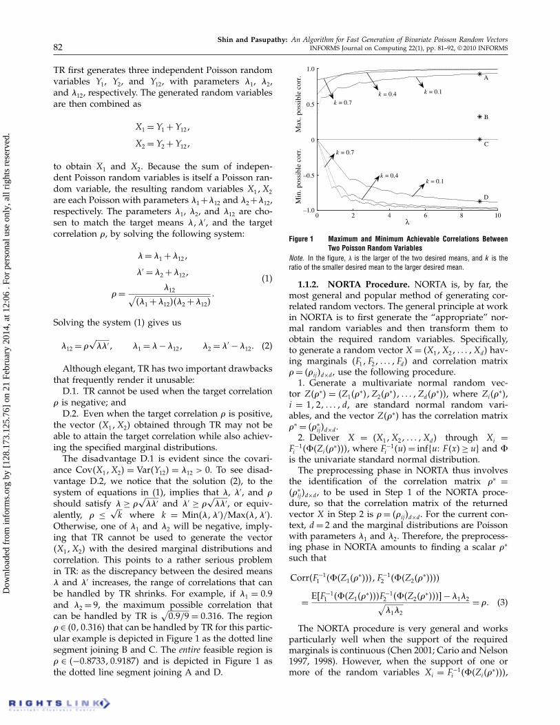
� ∈ �0�0�316� that can be handled by TR for this partic-ular example is depicted in Figure 1 as the dotted linesegment joining B and C. The entire feasible region is� ∈ �−0�8733�0�9187� and is depicted in Figure 1 asthe dotted line segment joining A and D.

0 2 4 6 8 10–1.0

–0.5

0

0.5

1.0A

B

C

D

λ

Min

. pos

sibl

e co

rr.

k = 0.7k = 0.4 k = 0.1

k = 0.7

k = 0.4k = 0.1

Max

. pos

sibl

e co

rr.

Figure 1 Maximum and Minimum Achievable Correlations BetweenTwo Poisson Random Variables

Note. In the figure, � is the larger of the two desired means, and k is theratio of the smaller desired mean to the larger desired mean.

1.1.2. NORTA Procedure. NORTA is, by far, themost general and popular method of generating cor-related random vectors. The general principle at workin NORTA is to first generate the “appropriate” nor-mal random variables and then transform them toobtain the required random variables. Specifically,to generate a random vector X = �X1�X2� � � � �Xd� hav-ing marginals �F1� F2� � � � � Fd� and correlation matrix�= ��ij �d×d, use the following procedure.1. Generate a multivariate normal random vec-

tor Z��∗� = �Z1��∗��Z2��∗�� � � � �Zd��

∗��, where Zi��∗�,

i = 1�2� � � � � d, are standard normal random vari-ables, and the vector Z��∗� has the correlation matrix�∗ = ��∗

ij �d×d.2. Deliver X = �X1�X2� � � � �Xd� through Xi =

F −1i ���Zi��

∗���, where F −1i �u�= inf�u� F �x�≥ u� and �

is the univariate standard normal distribution.The preprocessing phase in NORTA thus involves

the identification of the correlation matrix �∗ =��∗

ij �d×d, to be used in Step 1 of the NORTA proce-dure, so that the correlation matrix of the returnedvector X in Step 2 is �= ��ij �d×d. For the current con-text, d= 2 and the marginal distributions are Poissonwith parameters �1 and �2. Therefore, the preprocess-ing phase in NORTA amounts to finding a scalar �∗

such that

Corr�F −11 ���Z1��

∗���� F −12 ���Z2��

∗����

= E�F −11 ���Z1��

∗���F −12 ���Z2��

∗���−�1�2√�1�2

= �� (3)

The NORTA procedure is very general and worksparticularly well when the support of the requiredmarginals is continuous (Chen 2001; Cario and Nelson1997, 1998). However, when the support of one ormore of the random variables Xi = F −1

i ���Zi��∗���,

Dow

nloa

ded

from

info

rms.

org

by [

128.

173.

125.

76]

on 2

1 Fe

brua

ry 2

014,

at 1

2:06

. Fo

r pe

rson

al u

se o

nly,

all

righ

ts r

eser

ved.

Shin and Pasupathy: An Algorithm for Fast Generation of Bivariate Poisson Random VectorsINFORMS Journal on Computing 22(1), pp. 81–92, © 2010 INFORMS 83

i= 1�2, is denumerable (countably infinite) as in thecurrent context, the root-finding problem (3) turnsout to be nontrivial and difficult to solve efficiently.As elaborated in Avramidis et al. (2009), the maindifficulty lies in efficiently and accurately computingthe function g��∗� = E�F −1

1 ���Z1��∗���F −1

2 ���Z2��∗���,

which, in the denumerable case, turns out to bean infinite double sum with the summand being abivariate normal tail probability. We say more on thisin §5.2, where we discuss a fast implementation ofNORTA and compare it with that of the proposedalgorithm.

1.2. ContributionsIn this paper, we extend TR appropriately to proposeTREx—a tailored algorithm for generating bivariatePoisson random vectors. The following are specificcontributions of this work.1. We characterize and depict the theoretical limits

of the feasible range of correlations for a given pair ofPoisson distributions (§2, Propositions 1–5).2. We describe and list TREx, an algorithm for gen-

erating correlated Poisson random vectors (§3). Thealgorithm is exact and covers all theoretically feasiblecorrelations in two dimensions. We detail a fast algo-rithm for solving the preprocessing phase in TREx,along with directives on implementation (§4).3. We provide rigorous bounds for truncation error

control (§4.2, Propositions 9 and 10) useful for TREximplementation.4. A minor contribution is obtaining bounds for the

error incurred in truncating the double infinite sumwhen computing E�F −1

1 ���Z1��∗���F −1

2 ���Z2��∗���

within NORTA (Proposition 11). Although we presentthis bound for the Poisson case in §5, it may beuseful in other NORTA contexts where the marginaldistributions are denumerable.5. All code is available at https://filebox.vt.edu/

users/pasupath/pasupath.htm. Specifically, the web-site provides (i) a fast module (“maxcorr”) that calcu-lates the maximum and minimum allowable correla-tion between any two Poisson random variables, and(ii) an implementation of TREx that incorporates theerror bounds detailed in the paper.

1.3. OrganizationThe remainder of the paper is organized as fol-lows. In §2 we characterize the structure of thefeasible region of correlations between two Poissonrandom variables as a function of the Poisson param-eters �1��2. In §3, we present a detailed descriptionand listing of the TREx algorithm. This is followedby §4, where we provide an algorithm for executingthe preprocessing phase of TREx, including directiveson implementation. Section 5 describes results fromextensive numerical tests on the preprocessing phasesof TREx and NORTA. We provide concluding remarksin §6.

2. Structure of the Feasible RegionIn this section, we depict the feasible set of correla-tions between two Poisson random variables X1�X2with respective parameters ���′. We first presentthe following definition introduced by Ghosh andHenderson (2003).Definition 1. A product-moment (rank) correla-

tion matrix � is feasible for a given set of marginaldistributions F1� F2� � � � � Fd if there exists a random vec-tor X with marginal distributions F1� F2� � � � � Fd andproduct-moment (rank) correlation matrix �.To illustrate feasible correlation matrices, consider

two Poisson random variables X1 and X2 havingrespective means � = 0�5 and �′ = 0�5. It can beshown that the largest achievable positive correla-tion between X1 and X2 is 1, and the largest achiev-able negative correlation between X1 and X2 is −0�5.Therefore, any correlation matrix

�=(1 rr 1

)�

with r values in the interval �−0�5�1 is a feasible cor-relation matrix for the vector �X1�X2�. The matrix �is a correlation matrix, but not feasible, if r lies in theinterval �−1�−0�5�.More generally, as shown in Whitt (1976), if ran-

dom variables X1 and X2 have cumulative distri-bution functions (cdfs) F �x� and G�x�, respectively,and U is a random variable that is uniformly dis-tributed between 0 and 1, then Corr�F −1�U��G−1�U��is the maximum achievable and Corr�F −1�U��G−1�1−U�� the minimum achievable correlations between X1and X2, respectively. Therefore the feasible set of cor-relations between the random variables X1 and X2 is�Corr�F −1�U��G−1�1−U���Corr�F −1�U��G−1�U��.Figure 1 depicts this feasible set when X1 and X2 are

Poisson random variables. The figure is plotted as afunction of the larger desired mean � (assumed with-out loss of generality) of X1 and X2, and the ratio k ofthe smaller to the larger desired means of X1 and X2.Thus, for a given � and k, a vertical line betweenthe corresponding upper and lower curves depicts therange of feasible correlations.Five properties of the curves depicted in Figure 1

are noteworthy.—Each curve is continuous everywhere in � ∈ �0� �

(Proposition 1). Furthermore, the set of points whereeach curve is nondifferentiable has Lebesgue measurezero (Proposition 7).—There is an initial linear region for every negative

correlation curve (see the bottom half of Figure 1).This corresponds to the region ��� F −1

� �u�F −1k� �1−u�= 0

for all u ∈ �0�1}.—For a given ratio of the two parameters, i.e., for

fixed k, the maximum positive andmaximum negativecorrelations tend to 1 and −1, respectively, as �→ (Proposition 3).

Dow

nloa

ded

from

info

rms.

org

by [

128.

173.

125.

76]

on 2

1 Fe

brua

ry 2

014,

at 1

2:06

. Fo

r pe

rson

al u

se o

nly,

all

righ

ts r

eser

ved.

Shin and Pasupathy: An Algorithm for Fast Generation of Bivariate Poisson Random Vectors84 INFORMS Journal on Computing 22(1), pp. 81–92, © 2010 INFORMS

—The curves are in the form of “scallops” with theends of the scallops corresponding to the points ofnondifferentiability.—The curves become “approximately linear” when

multiplied by the factor �√k.

Propositions 1 through 5 characterize the limitingbehavior of these curves rigorously. As stated ear-lier, assume X1 and X2 are Poisson random vari-ables with means � and �′. Also assume, without lossin generality, that � ≥ �′. Denote the maximum andminimum achievable correlation between X1 and X2as �+����′� and �−����′�, respectively. Also, denotek= �′/�. Proofs for Propositions 1 through 5 areprovided in the Online Supplement (available athttp://joc.pubs.informs.org/ecompanion.html).

Proposition 1. Functions �+���k��, �−���k�� arecontinuous in ���k� ∈ �0� �× �0�1.

Proposition 2. For fixed k,

lim�→0

�+���k��=√k� lim

�→0�−���k��= 0�

Proposition 3. For fixed k,

lim�→

�+���k��= 1� lim�→

�−���k��=−1�

Proposition 4. For fixed �,

limk→0

�+���k��= 0� limk→0

�−���k��= 0�

Proposition 5. For fixed �,

limk→1

�+���k��= �+������ limk→1

�−���k��= �−������

3. TREx—Algorithm DescriptionRecall that the objective is to generate the randomvector �X1�X2� such that X1 has a Poisson distribu-tion with mean �, X2 has a Poisson distribution withmean �′, and Corr�X1�X2� = �, where ���′ > 0 and� ∈ �−1�1� are given.Our assumption about � ∈ �−1�1� creates the pos-

sibility of the desired correlation being infeasible; i.e.,� > �+���k�� or � < �−���k��. This problem of infea-sibility is not a complication because it is automat-ically detected at the end of the preprocessing step.In other words, the proposed algorithm is such thatnothing special needs to be done to check for an infea-sible problem.Denote F −1

� �y�= inf�x � F��x� > y�, where F��x� is thePoisson cdf with mean �. Let U be a random variablethat is uniformly distributed between 0 and 1. Thenthe proposed algorithm takes the following form:

X1=Y1+F −1�∗ �U�� X2=Y2+F −1

k�∗�U� if �>0�

X1=Y1+F −1�∗ �U�� X2=Y2+F −1

k�∗�1−U� if �<0�(4)

We draw attention to three aspects of the proposedoperations. First, when �> 0, i.e., when positive corre-lation between X1 and X2 is sought, we use commonrandom numbers as in TR. When � < 0, we use anti-thetic variates to induce negative correlation betweenX1 and X2. Second, we note that for both cases, �> 0and � < 0, unlike TR, there is no “common randomvariable.” Instead, the random variables inducing cor-relation are obtained through inversion of two differ-ent Poisson cdfs. The means of these Poisson cdfs arein the same ratio as the target means � and �′. Third,the value of �∗ needs to be determined as part of thepreprocessing step so that the resulting random vari-ables X1, X2 attain the target means and the targetcorrelation.

3.1. TREx—Algorithm ListingWe list the operations involved in TREx as Algo-rithm 1. We discuss Step 7 (preprocessing step) indetail in §4. Inverting a Poisson cdf, required invarious steps, can be done efficiently through exist-ing random variate generation routines (Kemp andKemp 1991, Schmeiser and Kachitvichyanukul 1981,Devroye 1986).

Algorithm 1 (TREx)Require: �> 0��′ > 0�� ∈ �−1�1�1: if �= 0 then2: Generate U1 ∼U�0�1�, U2 ∼U�0�1�,

independently3: X1 ← F −1

� �U1�4: X2 ← F −1

�′ �U2�5: return �X1�X2�6: end if7: Solve for �∗ {preprocessing step}8: Generate U1 ∼U�0�1�, U2 ∼U�0�1�, U3 ∼U�0�1�independently

9: Y1 ← F −1�−�∗�U1�

10: Y2 ← F −1�′−k�∗�U2�

11: Y12 ← F −1�∗ �U3�

12: if �> 0 then13: Y ′

12 ← F −1k�∗�U3�

14: else15: Y ′

12 ← F −1k�∗�1−U3�

16: end if17: X1 ← Y1+Y1218: X2 ← Y2+Y ′

1219: return �X1�X2�

3.2. RationaleIt is clear that TREx addresses the disadvantage D.1in TR. What is not immediately evident is the fact thatTREx fully addresses disadvantage D.2 as well. To seethis, consider the �> 0 operation in (4). It is clear fromconstruction that the random variables Y1, Y2, F −1

�∗ �U�,and F −1

k�∗�U� are each Poisson distributed with respec-tive means � − �∗, �′ − k�∗, �∗, and k�∗. Therefore,

Dow

nloa

ded

from

info

rms.

org

by [

128.

173.

125.

76]

on 2

1 Fe

brua

ry 2

014,

at 1

2:06

. Fo

r pe

rson

al u

se o

nly,

all

righ

ts r

eser

ved.

Shin and Pasupathy: An Algorithm for Fast Generation of Bivariate Poisson Random VectorsINFORMS Journal on Computing 22(1), pp. 81–92, © 2010 INFORMS 85

the random variables X1 and X2 will have the correctmarginal distributions, provided the quantities �−�∗

and �′ − k�∗ remain positive. This, however, can beensured by restricting �∗ to the interval �0��, afterrecalling that � ≥ �∗ and k ≤ 1. A similar argumentholds for the �< 0 case as well.What range of correlations are covered if we restrict

�∗ to the interval �0��? To answer this question, againconsider the � > 0 case in (4). As �∗ → 0, we haveCorr�X1�X2� → 0, giving us the trivial uncorrelatedcase. On the other extreme, as �∗ → �, we have � −�∗ → 0, �′ − k�∗ → 0, and k�∗ → �′. These threeimplications together mean that Y1 and Y2 vanish,and Corr�X1�X2�→Corr�F −1

� �U�� F −1k� �U��= �+���k��.

Furthermore, it can be shown that Corr�X1�X2� isa continuous function of �∗. These three facts—Corr�X1�X2�→ 0 as �∗ → 0, Corr�X1�X2�→ �+���k��as �∗ → �, and the continuity of Corr�X1�X2� as a func-tion of �∗—ensure that the entire range of positivecorrelations �0��+���k�� can be achieved throughTREx. Similar arguments for the �< 0 case imply thatTREx achieves the entire range of negative correlations��−���k���0 as well.Before we state the above arguments formally

through Proposition 6, we also note in passing that wecan achieve a similar effect, i.e., obtaining the entirerange of feasible correlations, through

X1=Y1+F −1�∗1

�U�� X2=Y2+F −1�∗2

�U� if �>0�

X1=Y1+F −1�∗1

�U�� X2=Y2+F −1�∗2

�1−U� if �<0�(5)

instead of (4). The operation (5), however, providesno advantages over (4), at least in two dimensions.It does have the disadvantage of making the prepro-cessing step a two-dimensional search, as opposedto the one-dimensional search afforded by (4). Theproof of Proposition 6 is a simple consequence ofProposition 1.

Proposition 6. Let Y1, Y2 be Poisson random variableswith means �− �∗ and �′ − k�∗, respectively, where 0 <�∗ ≤ � and k = �′/� ≤ 1. Let U be a random variablethat is mutually independent of Y1 and Y2, and uniformlydistributed between 0 and 1. Then(i) the functions Corr�Y1 + F −1

�∗ �U��Y2 + F −1k�∗�U��,

Corr�Y1 + F −1�∗ �U��Y2 + F −1

k�∗�1 − U�� are continuous in�∗ ∈ �0��;(ii) lim�∗→�Corr�Y1 + F −1

�∗ �U��Y2 + F −1k�∗�U�� =

�+���k��� and(iii) lim�∗→�Corr�Y1 + F −1

�∗ �U��Y2 + F −1k�∗�1 − U�� =

�−���k���

4. TREx Preprocessing Step(Solving for �∗)

We see from (4) that X1 and X2 have the cor-rect marginal distributions. The more challenging

0 5 10 15 20 25–25

–20

–15

–10

–5

5

10

15

20

25

x

k = 0.7

k = 0.4

k = 0.1

k = 0.7

k = 0.4

k = 0.1

x = λ*

ρ

ρ

x = λ*

Cov

(Fλ–1

(U),

F kλ–1

Cov

(Fλ–1

(U),

F kλ

(1–U

))–1

(U))

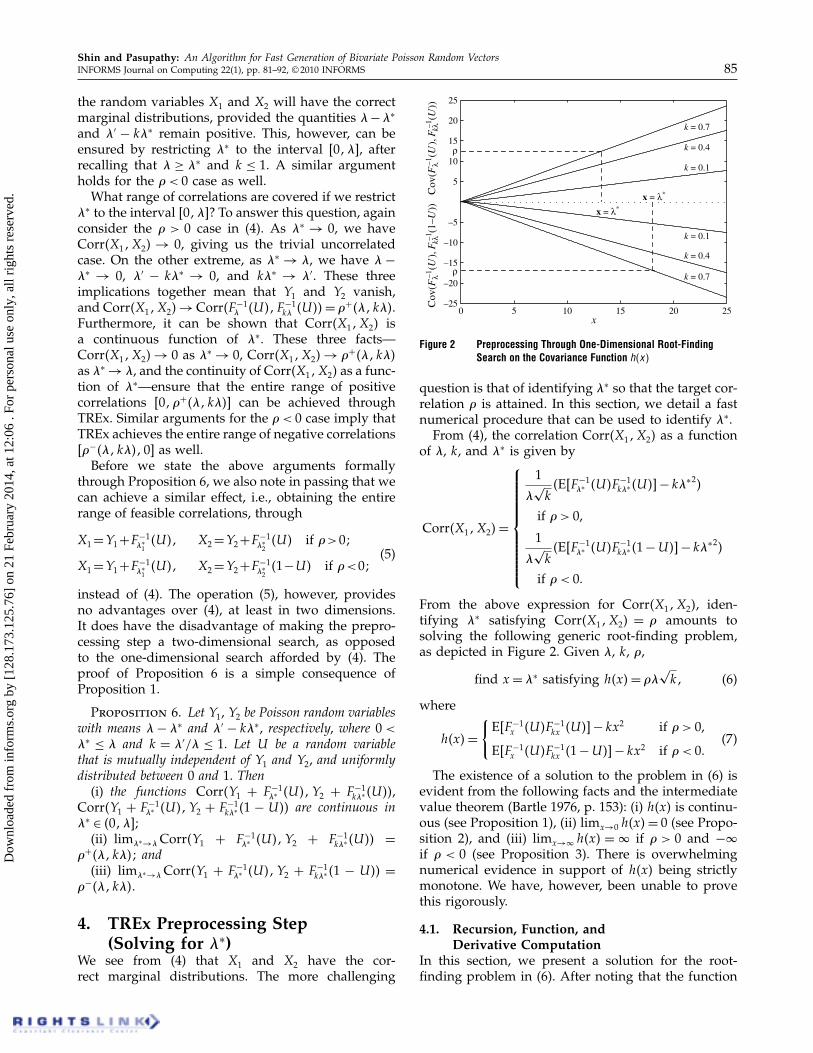
Figure 2 Preprocessing Through One-Dimensional Root-FindingSearch on the Covariance Function h�x�

question is that of identifying �∗ so that the target cor-relation � is attained. In this section, we detail a fastnumerical procedure that can be used to identify �∗.From (4), the correlation Corr�X1�X2� as a function

of �, k, and �∗ is given by

Corr�X1�X2�=

1

�√k�E�F −1

�∗ �U�F −1k�∗�U�− k�∗2�

if �> 0,

1

�√k�E�F −1

�∗ �U�F −1k�∗�1−U�− k�∗2�

if �< 0.

From the above expression for Corr�X1�X2�, iden-tifying �∗ satisfying Corr�X1�X2� = � amounts tosolving the following generic root-finding problem,as depicted in Figure 2. Given �, k, �,

find x= �∗ satisfying h�x�= ��√k� (6)

where

h�x�={E�F −1

x �U �F −1kx �U �− kx2 if �> 0,

E�F −1x �U �F −1

kx �1−U�− kx2 if �< 0.(7)

The existence of a solution to the problem in (6) isevident from the following facts and the intermediatevalue theorem (Bartle 1976, p. 153): (i) h�x� is continu-ous (see Proposition 1), (ii) limx→0 h�x�= 0 (see Propo-sition 2), and (iii) limx→ h�x� = if � > 0 and − if � < 0 (see Proposition 3). There is overwhelmingnumerical evidence in support of h�x� being strictlymonotone. We have, however, been unable to provethis rigorously.

4.1. Recursion, Function, andDerivative Computation

In this section, we present a solution for the root-finding problem in (6). After noting that the function

Dow

nloa

ded

from

info

rms.

org

by [

128.

173.

125.

76]

on 2

1 Fe

brua

ry 2

014,

at 1

2:06

. Fo

r pe

rson

al u

se o

nly,

all

righ

ts r

eser

ved.

Shin and Pasupathy: An Algorithm for Fast Generation of Bivariate Poisson Random Vectors86 INFORMS Journal on Computing 22(1), pp. 81–92, © 2010 INFORMS

h is differentiable almost everywhere through Propo-sition 7, we detail the efficient computation of h�x�and its derivative h′�x�, and provide rigorous direc-tives on safely truncating the summations that appearduring their computation.

Proposition 7. The real-valued function

h�x�={E�F −1

x �U �F −1kx �U �− kx2 if �> 0,

E�F −1x �U �F −1

kx �1−U�− kx2 if �< 0

is differentiable almost everywhere.

Proof. Since the products F −1x �U �F −1

kx �U � andF −1x �U �F −1

kx �1 − U� are each nondecreasing in x(for fixed U ), the functions E�F −1

x �U �F −1kx �U � and

E�F −1x �U �F −1

kx �1 − U� are both nondecreasing in x.This implies, however, that E�F −1

x �U �F −1kx �U � and

E�F −1x �U �F −1

kx �1− U� are differentiable almost every-where (Royden 1988, p. 100). Conclude that h�x� isdifferentiable almost everywhere. �

For solving the root-finding problem (6), we use aNewton recursion on h�x�:

x= x+ 1h′�x�

���√k−h�x��� (8)

In what follows, we elaborate on the efficient compu-tation of h�x�, h′�x� appearing in (8).

Case � < 0: When � < 0, we note that E�F −1x �U � ·

F −1kx �1− U� = 0 when x is small enough, i.e., if Fx�0�+Fkx�0� = e−x + e−kx ≥ 1� In such a case, h�x� = −kx2

implies that �∗ =√−��/

√k. Otherwise, we compute

h�x� = ∫ 10 F

−1x �u�F −1

kx �1 − u�du − kx2 starting from the“middle region” of the integral and progressivelysumming out to the tails.To do this, we first compute mx = Min�k ∈ Z+�

Fx�k� ≥ 0�5��mkx = Min�k ∈ Z+� Fkx�k� ≥ 0�5�,and the corresponding cumulative probabilitiesFx�mx�� Fkx�mkx�, where Z+ = �0�1�2� � � �� denotes theset of nonnegative integers. An efficient way tocompute these is through J -fraction approximationsgiven in Kemp (1988). These approximations arehighly accurate analytic expressions for Fx�r�, wherer is the “round-off” value of x, i.e., the integer thatsatisfies r +%= x�−0�5≤ %< 0�5. We then express

h�x� =∫ 0�5

0F −1x �u�F −1

kx �1−u�du

+∫ 0�5

0F −1kx �u�F −1

x �1−u�du− kx2� (9)

The first of the integrals on the right-hand side of (9)is 0 if mx = 0. Otherwise,

∫ 0�5

0F −1x �u�F −1

kx �1−u�du= S+ ∑j=mx−1�mx−2� ����1

Sj� (10)

where

lj = Min�n ∈Z+ � 1− Fkx�n�≤ Fx�j��� for j = 1�2� � � � �

Sj =

jlj �Fx�j�− Fx�j − 1��� if 1− Fkx�lj � < Fx�j − 1��

Bj +Cj +lj−1−2∑i=lj

Tij � otherwise�

Bj = jlj �Fx�j�− 1+ Fkx�lj ���Cj = jlj−1�1− Fkx�lj−1− 1�− Fx�j − 1���Tij = �i+ 1�j�Fkx�i+ 1�− Fkx�i���

S =

mxmkx�0�5− Fx�mx − 1���if 1−Fkx�mkx�≤Fx�mx−1��

B+C +lmx−1−2∑i=mkx

Timx� otherwise�

B= mxmkx�Fkx�mkx�− 0�5��C = mxlmx−1�1− Fkx�lmx−1− 1�− Fx�mx − 1��.The expression in (10) is obtained upon noting thatthe function F −1

x �u� takes the value mx −1 in the inter-val �Fx�mx − 1��0�5, mx − 2 in the interval �Fx�mx − 2��Fx�mx − 1��, mx − 3 in the interval �Fx�mx − 3��Fx�mx−2��, and so on. Similarly, the function F −1

kx �1−u�takes the value mkx in the interval �1− Fkx�mkx��0�5,mkx + 1 in the interval �1− Fkx�mkx + 1�� 1− Fkx�mkx��,mkx+2 in the interval �1−Fkx�mkx+2�� 1−Fkx�mkx+1��,and so on. The integral on the left-hand side of (10)can thus be expressed as a summation by splitting theinterval �0�0�5 into sub-intervals starting from 0�5 andobtained by arranging the numbers 0�5� Fx�mx−1�� 1−Fkx�mkx�� Fx�mx−2�� 1−Fkx�mkx+1�� � � � � in descendingorder. The first such subinterval gives rise to the sum-mand S as defined, and the (j + 1)th subinterval givesrise to the summand Sj as defined. (The summation onthe right-hand side of (10) has only a finite number ofterms because F −1

x �u� = 0 for u ∈ �0� Fx�0�.) A similarcalculation applies to the second integral appearing onthe right-hand side of (9) and for the expressions in(12) and (13) below.

Case � > 0: For this case, unlike the � < 0 case,there exists no linear portion of the curves in Figure 1.Again, we first compute mx = Min�k ∈ Z+� Fx�k� ≥0�5��mkx = Min�k ∈ Z+� Fkx�k� ≥ 0�5�, and the cor-responding cumulative probabilities Fx�mx�� Fkx�mkx�using the J -fraction approximations in Kemp andKemp (1991). We again express h�x� in two parts as

h�x� =∫ 0�5

0F −1x �u�F −1

kx �u�du

+∫ 1

0�5F −1x �u�F −1

kx �u�du− kx2� (11)

The first of the integrals in (11) is 0 if either mx = 0 ormkx = 0. Otherwise,∫ 0�5

0F −1x �u�F −1

kx �u�du= S+ ∑j=mx−1�mx−2� ����1

Sj� (12)

Dow

nloa

ded

from

info

rms.

org

by [

128.

173.

125.

76]

on 2

1 Fe

brua

ry 2

014,

at 1

2:06

. Fo

r pe

rson

al u

se o

nly,

all

righ

ts r

eser

ved.

Shin and Pasupathy: An Algorithm for Fast Generation of Bivariate Poisson Random VectorsINFORMS Journal on Computing 22(1), pp. 81–92, © 2010 INFORMS 87

where

lj = Max�n∈Z+� Fkx�n�≤Fx�j��� for j=1�2�����

Sj =

j�lj+1��Fx�j�−Fx�j−1��� if Fkx�lj �<Fx�j−1��

Bj+Cj+lj−1+2∑i=lj

Tij � otherwise�

Bj = j�lj+1��Fx�j�−Fkx�lj ���

Cj = j�lj−1+1��Fkx�lj−1+1�−Fx�j−1���Tij = ji�Fkx�i�−Fkx�i−1���

S =

mxmkx�0�5−Fx�mx−1���if Fkx�mkx−1�≤Fx�mx−1��

B+C+lmx−1+2∑i=mkx−1

Timx� otherwise�

B = mxmkx �0�5−Fkx�mkx−1���C = mx�lmx−1+1��Fkx�lmx−1+1�−Fx�mx−1���

Similarly, the second integral on the right-hand sideof (11) can be written as

∫ 1

0�5F −1x �u�F −1

kx �u�du= S+ ∑

j=mx+1Sj� (13)

where

lj = Max�n ∈Z+� Fkx�n�≤ Fx�j��� for j = 1�2� � � � �

Sj =

j�lj + 1��Fx�j�− Fx�j − 1��� if Fkx�lj � < Fx�j − 1��

Bj +Cj +lj−1∑

i=lj−1+1Tij� otherwise�

Bj = j�lj + 1��Fx�j�− Fkx�lj ���

Cj = j�lj−1+ 1�(Fkx�lj−1+ 1�− Fx�j − 1�

)�

Tij = j�i+ 1��Fkx�i+ 1�− Fkx�i���

S =

mxmkx�Fx�mx�− 0�5�� if Fkx�mkx�≥ Fx�mx��

B+C +lmx

−1∑i=mkx

Timx� otherwise�

B = mx�lmx+ 1��Fx�mx�− Fkx�lmx���

C = mxmkx�Fkx�mkx�− 0�5��

The derivative h′�x� can be obtained through directdifferentiation of the summation expressions forh�x�, after noting the derivatives (with respect to x)

F ′x�0� = −e−x, F ′

kx�0� = −ke−kx, and F ′x�i� =

−Px�i�� F′kx�i�=−kPkx�i� for i= 1�2� � � � �

4.2. Bounds on Truncation ErrorAs described in §4.1, computing h�x� is based on asummation involving a potentially large number oftail probabilities from specified Poisson distributions.From a computational standpoint, it would be usefulto truncate this summation, while making sure thatthe terms excluded add to less than a prespecified tol-erance -. In this section, we present results that pro-vide directives for such safe truncation. We first notethe following identities related to the moments of thePoisson distribution. See the Online Supplement for aproof.

Proposition 8. Let Px and Fx denote the probabil-ity mass function and cumulative distribution function,respectively, of the Poisson distribution with mean x. Then,(i)

∑ j=s jPx�j�= x�1− Fx�s− 2��� s ∈Z;

(ii)∑

j=s j2Px�j�= x2�1− Fx�s− 3��+ x�1− Fx�s− 2���

s ∈Z;(iii)

∑sj=0 j

2Px�j�= x2�Fx�s− 2��+ x�Fx�s− 1��� s ∈Z.

Recall that when � < 0, we wrote h�x� =∫ 0�50 F −1

x �u�F −1kx �1 − u�du + ∫ 0�5

0 F −1kx �u�F −1

x �1 − u�du. Wealso expressed each of these integrals through a dou-ble summation (10) that starts from the center, i.e.,from u = 0�5, and sums outward to u = 0. Proposi-tion 9, proved in the Online Supplement, provides abound on the error because of truncating each of thesesummations.

Proposition 9. Let Fx and Fkx represent Poisson cdfswith respective means x and kx. Then,∣∣∣∣

∫ 0�5

0F −1x �u�F −1

kx �1−u�du−∫ 0�5

/F −1x �u�F −1

kx �1−u�du

∣∣∣∣≤ F −1

x �/�kx�1− Fkx�F−1kx �1− /�− 3��� (14)

In illustrating the usefulness of Proposition 9, sup-pose that we have summed to u = / > 0 and thatour required tolerance in computing h�x� is -. Then,apply the error bound in (14) to each integral com-prising h�x� individually by stopping the summa-tion when the right-hand side of (14) falls below -/2.Because every term in the right-hand side of (14) isknown, checking the error bound is also computation-ally cheap.We next present a similar truncation error bound

for the �> 0 case. Recall that for the �> 0 case, h�x�=∫ 0�50 F −1

x �u�F −1kx �u�+ ∫ 1

0�5 F−1x �u�F −1

kx �u�, with the individ-ual integrals being expressed as double summationsshown in (12) and (13). Proposition 10 provides sep-arate truncation error bounds for these, with a proofin the Online Supplement.

Dow

nloa

ded

from

info

rms.

org

by [

128.

173.

125.

76]

on 2

1 Fe

brua

ry 2

014,

at 1

2:06

. Fo

r pe

rson

al u

se o

nly,

all

righ

ts r

eser

ved.

Shin and Pasupathy: An Algorithm for Fast Generation of Bivariate Poisson Random Vectors88 INFORMS Journal on Computing 22(1), pp. 81–92, © 2010 INFORMS

Proposition 10. Let Fx and Fkx represent Poisson cdfswith respective means x and kx. Then,(i) ∣∣∣∣

∫ 0�5

0F −1x �u�F −1

kx �u�du−∫ 0�5

/F −1x �u�F −1

kx �u�du

∣∣∣∣≤√I�x� F −1

x �/��I�kx� F −1kx �/���

where I�x�y�= x2Fx�y− 2�+ xFx�y− 1�.(ii)∣∣∣∣

∫ 1

0�5F −1x �u�F −1

kx �u�du−∫ 1−/

0�5F −1x �u�F −1

kx �u�du

∣∣∣∣≤√I ′�x� F −1

x �1− /�− 1�I ′�kx� F −1kx �1− /�− 1��

where I ′�x�y�= x2�1− Fx�y− 3��+ x�1− Fx�y− 2��.Proposition 10, in a fashion similar to Proposi-

tion 9, suggests that we do not have to include allthe summands appearing in (12) and (13). Instead, if- is the prescribed tolerance, stop the summation for∫ 0�50 F −1

x �u�F −1kx �u�duwhen I�x� F −1

x �/�� and I�kx� F −1kx �/��

each fall below√-/2. Similarly, stop the summation

for∫ 10�5 F

−1x �u�F −1

kx �u�du when I ′�x� F −1x �1−/� − 1� and

I ′�kx� F −1kx �1− /�− 1� each fall below √

-/2.

4.3. Initial GuessMotivated by Figure 2, the initial guess x0 for therecursion (8) is obtained through a linear approxi-mation l�x� to the function h�x�. From Proposition 3,we see that for fixed k,

limx→

E�F −1x �U �F −1

kx �U �− kx2

x=√

k�

limx→

E�F −1x �U �F −1

kx �1−U�− kx2

x=−√

k�

Thus, for a given problem instance, the initial guess x0for the recursion (8) is obtained by solving for x fromthe equation l�x�= sign���

√k x+ c = ��

√k, to obtain

x0 = ���√k−c�/�sign���

√k�. The intercept c of the lin-

ear approximation l�x� is set heuristically. For instance,we recommend c = 0 for � > 0, and c = √

kbm − kb2mfor � < 0, where bm is the boundary of the “initial lin-ear region” for the negative correlation case. Recallthat the boundary bm is the solution to the equatione−bm +e−kbm = 1 and can be obtained rapidly through aNewton search.We conclude this section with Algorithm 2—a for-

mal algorithm listing of the preprocessing step inTREx.

Algorithm 2 (TREx preprocessing step)

Require: �1 > 0��2 > 0�−1≤ �≤ 1� - > 01: if ��� ≤ - then2: return 0 {i.e., generate independently}

3: end if4: �←Max��1��2�5: k←Min��1��2�/�6: s← sign���

√k

7: if �< 0 then8: Solve for bm to within tolerance - {i.e., find bm

satisfying e−bm + e−kbm = 1}9: if �

√k�≥−kb2m then

10: return√−��/

√k {solution lies in the initial

linear region}11: end if12: c←√

kbm − kb2m13: else14: c← 015: end if16: �∗ = ��

√k�− c�/s {initial guess}

17: �̂← 018: while ��̂−��> - do19: Calculate �∗��∗

1

�∗ = �+��∗� k�∗� if �> 0�= �−��∗� k�∗� if �< 0�

�∗1 =

d�∗

d�.

20: �̂= �∗�∗/�21: h′−1 ← �∗

1

√k�∗ +�∗√k

22: �∗←�∗+h′−1��√k�−�̂

√k�∗� {Newton update}

23: end while

5. Computational ExperienceRecall that both TREx and NORTA have two phases:(i) a preprocessing phase where the parametersrequired within the algorithm are identified, and (ii) ageneration phase where the identified parameters areused appropriately to generate the required Poissonrandom vector. In this section, we report detailedresults on execution times for (i). Our emphasis ison (i) because, as Table 1 demonstrates, TREx andNORTA are quite comparable in terms of executiontimes for (ii), with TREx being slightly faster.Recall from §1 that the Poisson random variate

generation problem has three problem parameters:the means �1��2 of the marginal distributions, anda desired correlation �. A problem is thus charac-terized uniquely by the three parameters ��1��2���,or equivalently by ���k���, where � = Max��1��2�and k = Min��1��2�/Max��1��2�. In assessing per-formance, a large number of pairs ����� were ran-domly generated at each of a set of fixed k valuesin �0�1, and phase (i) of both TREx and NORTAwere executed in MATLAB. The stipulated tolerancewas set at 10−4, and the tests were performed on anIntel 1.67 GHz processor. CPU execution times wererecorded using the “tic toc” function in MATLAB.All MATLAB code used in the numerical experiments

Dow

nloa

ded

from

info

rms.

org

by [

128.

173.

125.

76]

on 2

1 Fe

brua

ry 2

014,

at 1

2:06

. Fo

r pe

rson

al u

se o

nly,

all

righ

ts r

eser

ved.

Shin and Pasupathy: An Algorithm for Fast Generation of Bivariate Poisson Random VectorsINFORMS Journal on Computing 22(1), pp. 81–92, © 2010 INFORMS 89

Table 1 A Brief Comparison of the Generation Phases in the TREx andNORTA Algorithms

��1� �2� � TREx NORTA ��1� �2� � TREx NORTA

�1�1� 001 096 193 �10�25� 001 090 188020 089 185 020 113 188050 111 186 050 113 188090 089 185 090 113 188

�1�10� 001 089 186 �10�100� 001 102 189020 101 186 020 114 189050 101 186 050 114 189090 089 187 090 114 189

�1�25� 001 101 188 �25�25� 001 090 188020 101 187 020 112 188050 101 188 050 113 188090 101 191 090 113 188

�1�100� 001 102 188 �25�100� 001 102 190020 102 188 020 114 190050 102 188 050 114 190090 102 188 090 114 189

�10�10� 001 090 188 �100�100� 001 112 189020 111 188 020 114 189050 111 188 050 114 192090 111 188 090 113 189

Notes. The columns titled “TREx” and “NORTA” show the time, measured inseconds and excluding the preprocessing phase, required to generate 10,000two-dimensional Poisson random vectors with desired means ��1� �2� anddesired correlation �. As can be seen, both algorithms are comparable interms of generation times, with TREx being marginally faster. Our focusin this paper is more on the preprocessing phases of the two algorithms.

is available for download at https://filebox.vt.edu/users/pasupath/pasupath.htm.

5.1. TREx Preprocessing TimesFor assessing the efficiency of the preprocessing phasein TREx, roughly 500,000 pairs ����� were gener-ated randomly (uniformly) from the space �0�1�000×�−1�1� for each of the values k= 0�05�0�10� � � � �1. Ateach k value, the preprocessing phase in TREx wasthen executed, and the recorded CPU times were usedto estimate various quantiles. As noted earlier, we donot report generation times here, i.e., the time takento execute Steps 8 through 20 in the algorithm list-ing shown in §3.1. Results from the numerical exper-iments on TREx are depicted in Figure 3, where the25th, 50th, 75th, and 99th percentiles of executiontimes are plotted as a function of k.As can be seen from Figure 3, TREx exhibits uni-

formly fast preprocessing times. A majority of thegenerated problems are solved to stipulated tolerancewithin 8 × 10−4 CPU seconds. Among the roughly10 million problems that we generated in total, thepreprocessing phase for no problem took more than5 × 10−3 seconds and eight iterations. Figure 3 alsosuggests that problems that are symmetric in themeans of the required marginal distributions, i.e.,k ≈ 1, are somewhat easier to solve. This is becausethe shape of the correlation function is such that for

0 0.2 0.4 0.6 0.8 1.02

4

6

8

10

12× 10–4

k

CPU

tim

e (s

ecs.

)

Figure 3 Performance of the Preprocessing Phase in TRExNotes. The curves show the 25th, 50th, 75th, and 99th percentile prepro-cessing times estimated by randomly generating five hundred thousandproblems for each k = Min��1� �2�/Max��1� �2�. The reported CPU timeswere obtained from execution through a MATLAB compiler on an Intel1.67 GHz processor.

values of k close to 1, TREx’s initial guess detailed in§4.3 turns out to be quite accurate.Although we did not generate � values greater than

1,000, we do not see any reason why the proposedalgorithm will not work efficiently for larger � values.In such cases, however, it is worthwhile investigatingwhether a normal approximation to the Poisson is amore efficient alternative.

5.2. NORTA Preprocessing TimesAs suggested in §1.1.2, the NORTA procedure isvery general and works particularly well when thesupport of the required marginal distributions iscontinuous (Chen 2001; Cario and Nelson 1997,1998). However, as elaborated in Avramidis et al.(2009), when the support of one or more of themarginal distributions is denumerable, the root-finding problem (3) becomes nontrivial because ofthe difficulty in efficiently computing the functiong��∗� = E�F −1

1 ���Z1��∗���F −1

2 ���Z2��∗���. Avramidis

et al. (2009) alleviate this situation by noting that g��∗�and g′��∗� can be computed as

g��∗�= ∑i=0

∑j=0

���∗�zi� zj ��

g′��∗�= ∑i=0

∑j=0

4�∗�zi� zj ��

(15)

where ��∗�x�y� is the bivariate standard normaldistribution function and ���∗�x�y� = ��∗�−x�−y�,4�∗�x�y� is the bivariate normal density function withcorrelation �∗, zi =�−1�F1�i��, zj =�−1�F2�j��, and ��x�is the standard normal cdf.

Dow

nloa

ded

from

info

rms.

org

by [

128.

173.

125.

76]

on 2

1 Fe

brua

ry 2

014,

at 1

2:06

. Fo

r pe

rson

al u

se o

nly,

all

righ

ts r

eser

ved.

Shin and Pasupathy: An Algorithm for Fast Generation of Bivariate Poisson Random Vectors90 INFORMS Journal on Computing 22(1), pp. 81–92, © 2010 INFORMS

Various algorithms are outlined in Avramidis et al.(2009) for solving NORTA’s preprocessing phase.We report results from the execution of one ofthese algorithms—NI3—with which we had the mostsuccess. The NI3 algorithm, in essence, is the Newtoniteration (Ortega and Rheinboldt 1970):

�n+1 = �n −f ��n�

f ′��n�� f ��n�=

g��n�− k�2√k�

−�� (16)

with appropriate safeguards introduced to ensurethat the iterates stay within the stipulated range. Wealso tried two other algorithms—NI2A and NI2B—outlined in Avramidis et al. (2009), but we had muchless success primarily because of difficulties in reli-ably setting parameters within the embedded numer-ical integration procedure.In carrying out the recursion (16), we need to safely

approximate g��∗� and g′��∗� by truncating the infi-nite sums appearing in (15). We used the followingresult in deciding the number of summands to use inapproximating g��∗�.

Proposition 11. Let ��x� denote the univariate stan-dard normal cdf, let ��∗�x�y� denote the bivariate stan-dard normal cdf with correlation �∗, and let ���∗�x�y� =��∗�−x�−y�. Also, let zi = �−1�F1�i�� and zj =�−1�F2�j��, where F1� F2 are Poisson cdfs with parameters�1��2, respectively. Then,(i) if �∗ < 0,

∣∣∣∣ ∑i=0

∑j=0

���∗�zi� zj �−N∑i=0

N∑j=0

���∗�zi� zj �

∣∣∣∣≤ e−��1+�2�

sN

1− s�ee�1 + ee�2�

for all s�N satisfying 1> s ≥Max�e�1/N�e�2/N�;(ii) if �∗ > 0 and �1 ≥ �2 (without loss of generality),∣∣∣∣ ∑i=0

∑j=0

���∗�zi� zj �−N∑i=0

N∑j=0

���∗�zi� zj �

∣∣∣∣≤ 2e−N

((1�2

�2N + 3−�2�2+ ln�4�+ 2�1+

4�2

)e2�2

+�2N + 3�e2�1)+e�2 4

�2e−√

�N−1��2−2�1�2

·�1+√�N − 1��2− 2�1�2��

A bound on truncation error has been difficult toestablish for g′��∗�, although computing g′��∗� accu-rately is not needed for the Newton iterates in (16) toconverge. The bivariate cdf tail appearing as the sum-mand in (15) was calculated using the algorithm byGenz (2004), which appears to be the fastest amongthose available.

0 0.2 0.4 0.6 0.8 1.00

5

10

15

k

CPU

tim

e (s

ecs.

)

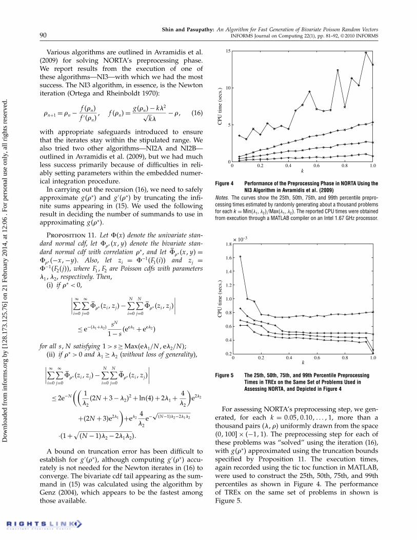
Figure 4 Performance of the Preprocessing Phase in NORTA Using theNI3 Algorithm in Avramidis et al. (2009)

Notes. The curves show the 25th, 50th, 75th, and 99th percentile prepro-cessing times estimated by randomly generating about a thousand problemsfor each k =Min��1� �2�/Max��1� �2�. The reported CPU times were obtainedfrom execution through a MATLAB compiler on an Intel 1.67 GHz processor.

0 0.2 0.4 0.6k

0.8 1.00.2

0.4

0.6

0.8

1.0

1.2

1.4

1.6

1.8× 10–3

CPU

tim

e (s

ecs.

)

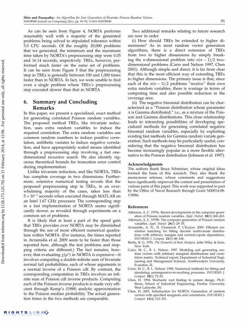
Figure 5 The 25th, 50th, 75th, and 99th Percentile PreprocessingTimes in TREx on the Same Set of Problems Used inAssessing NORTA, and Depicted in Figure 4

For assessing NORTA’s preprocessing step, we gen-erated, for each k = 0�05�0�10� � � � �1, more than athousand pairs ����� uniformly drawn from the space�0�100× �−1�1�. The preprocessing step for each ofthese problems was “solved” using the iteration (16),with g��∗� approximated using the truncation boundsspecified by Proposition 11. The execution times,again recorded using the tic toc function in MATLAB,were used to construct the 25th, 50th, 75th, and 99thpercentiles as shown in Figure 4. The performanceof TREx on the same set of problems in shown isFigure 5.

Dow

nloa

ded

from

info

rms.

org

by [

128.

173.

125.

76]

on 2

1 Fe

brua

ry 2

014,

at 1

2:06

. Fo

r pe

rson

al u

se o

nly,

all

righ

ts r

eser

ved.

Shin and Pasupathy: An Algorithm for Fast Generation of Bivariate Poisson Random VectorsINFORMS Journal on Computing 22(1), pp. 81–92, © 2010 INFORMS 91

As can be seen from Figure 4, NORTA performsreasonably well with a majority of the generatedproblems being solved to stipulated tolerance within5.0 CPU seconds. Of the roughly 20,000 problemsthat we generated, the minimum and the maximumtime taken by NORTA’s preprocessing step were 0�05and 16�14 seconds, respectively. TREx, however, per-formed much faster on the same set of problems.It can be seen from Figure 5 that the preprocessingstep in TREx is generally between 100 and 1,000 timesfaster than in NORTA. In fact, we were unable to findeven a single problem where TREx’s preprocessingstep executed slower than that in NORTA.

6. Summary and ConcludingRemarks

In this paper, we present a specialized, exact methodfor generating correlated Poisson random variables.The proposed method TREx, like trivariate reduc-tion, uses extra random variables to induce therequired correlation. The extra random variables usecommon random numbers to induce positive corre-lation, antithetic variates to induce negative correla-tion, and have appropriately scaled means identifiedthrough a preprocessing step involving a fast one-dimensional recursive search. We also identify rig-orous theoretical bounds for truncation error controlduring implementation.Unlike trivariate reduction, and like NORTA, TREx

has complete coverage in two dimensions. Further-more, extensive numerical testing reveals that theproposed preprocessing step in TREx, in an over-whelming majority of the cases, takes less than5× 10−3 seconds when executed through MATLAB onan Intel 1.67 GHz processor. The corresponding stepin a fast implementation of NORTA seems signifi-cantly slower, as revealed through experiments on acommon set of problems.It is likely that at least a part of the speed gain

that TREx provides over NORTA may be diminishedthrough the use of more efficient numerical quadra-ture within NORTA. (For instance, the times reportedin Avramidis et al. 2009 seem to be faster than thosereported here, although the test problems and stop-ping criteria are different.) The fact remains, how-ever, that evaluating g��∗� in NORTA is expensive—itinvolves computing a double-infinite sum of bivariatenormal tail probabilities, each of whose arguments isa normal inverse of a Poisson cdf. By contrast, thecorresponding computation in TREx involves an infi-nite sum of Poisson cdf inverse products. Computingeach of the Poisson inverse products is made very effi-cient through Kemp’s (1988) analytic approximationto the Poisson median probability. The actual genera-tion times in the two methods are comparable.

Two additional remarks relating to future researchare now in order.(i) How should TREx be extended to higher di-

mensions? As in most random vector generationalgorithms, there is a direct extension of TRExfrom two to higher dimensions by simply break-ing the n-dimensional problem into n�n − 1�/2 two-dimensional problems (Cario and Nelson 1997, Chen2001). Although simple and direct, it is far from clearthat this is the most efficient way of extending TRExto higher dimensions. The primary issue is that, sinceeach of the n�n− 1�/2 problems “receive” their ownextra random variables, there is wastage in terms ofcomputing time and also possible reduction in thecoverage area.(ii) The negative binomial distribution can be char-

acterized as a “Poisson distribution whose parameter� is Gamma distributed,” i.e., as a mixture of the Pois-son and Gamma distributions. This close relationshipleads to interesting possibilities of developing spe-cialized methods for generating correlated negativebinomial random variables, especially by exploitingexisting fast methods for Gamma random variate gen-eration. Such methods may be particularly useful, con-sidering that the negative binomial distribution hasbecome increasingly popular as a more flexible alter-native to the Poisson distribution (Johnson et al. 1997).

AcknowledgmentsThe authors thank Bruce Schmeiser, whose original ideasformed the basis of this research. They also thank theanonymous referees, whose comments and suggestionshave significantly improved the content and presentation ofvarious parts of this paper. This work was supported in partby the Office of Naval Research through Grant N00014-08-1-0066.

ReferencesAtkinson, A. C. 1979a. Recent developments in the computer gener-

ation of Poisson random variables. Appl. Statist. 28(3) 260–263.Atkinson, A. C. 1979b. The computer generation of Poisson random

variables. Appl. Statist. 28(1) 29–35.Avramidis, A. N., N. Channouf, P. L’Ecuyer. 2009. Efficient cor-

relation matching for fitting discrete multivariate distribu-tions with arbitrary margins and normal-copula dependence.INFORMS J. Comput. 21(1) 88–106.

Bartle, R. G. 1976. The Elements of Real Analysis. John Wiley & Sons,New York.

Cario, M. C., B. L. Nelson. 1997. Modeling and generating ran-dom vectors with arbitrary marginal distributions and corre-lation matrix. Technical report, Department of Industrial Engi-neering and Management Sciences, Northwestern University,Evanston, IL.

Cario, M. C., B. L. Nelson. 1998. Numerical methods for fitting andsimulating autoregressive-to-anything processes. INFORMS J.Comput. 10(1) 72–81.

Chen, H. 1994. Stochastic root finding in system design. Ph.D.thesis, School of Industrial Engineering, Purdue University,West Lafayette, IN.

Chen, H. 2001. Initialization for NORTA: Generation of randomvectors with specified marginals and correlations. INFORMS J.Comput. 13(4) 312–331.

Dow

nloa

ded

from

info

rms.

org

by [

128.

173.

125.

76]

on 2

1 Fe

brua

ry 2

014,

at 1

2:06

. Fo

r pe

rson

al u

se o

nly,

all

righ

ts r

eser

ved.

Shin and Pasupathy: An Algorithm for Fast Generation of Bivariate Poisson Random Vectors92 INFORMS Journal on Computing 22(1), pp. 81–92, © 2010 INFORMS

Devroye, L. 1986. Non-Uniform Random Variate Generation. Springer,New York.

Genz, A. 2004. Numerical computation of rectangular bivariate andtrivariate normal t probabilities. Statist. Comput. 14(3) 251–260.

Ghosh, S., S. G. Henderson. 2003. Behavior of the NORTA methodfor correlated random vector generation as the dimensionincreases. ACM TOMACS 13(3) 276–294.

Johnson, N. L., A. W. Kemp, S. Kotz. 2005. Univariate Discrete Dis-tributions. John Wiley & Sons, New York.

Johnson, N. L., S. Kotz, N. Balakrishnan. 1997. Discrete MultivariateDistributions. John Wiley & Sons, New York.

Kemp, A. W. 1988. Simple algorithms for the Poisson modalcumulative probability. Comm. Statist.: Simulation Comput. 17(4)1495–1508.

Kemp, C. D., A. W. Kemp. 1991. Poisson random variate generation.Appl. Statist. 40(1) 143–158.

Kronmal, R. A., A. V. Peterson Jr. 1979. On the alias method forgenerating random variables from a discrete distribution. Amer.Statistician 33(4) 214–218.

Mardia, K. V. 1970. Families of Bivariate Distributions. Griffin,London.

Ortega, J. M., W. C. Rheinboldt. 1970. Iterative Solution of NonlinearEquations in Several Variables. Academic Press, New York.

Royden, H. 1988. Real Analysis. Prentice Hall, New York.Schmeiser, B. W., V. Kachitvichyanukul. 1981. Poisson random vari-

ate generation. Technical report, School of Industrial Engineer-ing, Purdue University, West Lafayette, IN.

Shin, K., R. Pasupathy. 2007. A method for fast generation of bivari-ate Poisson random vectors. S. G. Henderson, B. Biller, M.-H.Hsieh, J. Shortle, J. D. Tew, R. R. Barton, eds. Proc. 2007 Win-ter Simulation Conf., Institute of Electrical and Electronics Engi-neers, Piscataway, NJ, 472–479.

Whitt, W. 1976. Bivariate distributions with given marginals. Ann.Statist. 4(6) 1280–1289.

Dow

nloa

ded

from

info

rms.

org

by [

128.

173.

125.

76]

on 2

1 Fe

brua

ry 2

014,

at 1

2:06

. Fo

r pe

rson

al u

se o

nly,

all

righ

ts r

eser

ved.