AEOC-TR-93-19 AD-A274 591

An Algorithm for Determination of Bearing Health

Through Automated Vibration Monitoring

9I S. W. Hite, IllSverdrup Technology/AEDC Group

December 1993

Final Report for Period October 1, 1992 - September 30, 1993

, DTIC -S ELECTE

JAN0 19941 DE

Approwd for public relese; distribution is unlimited.

94-00881

ARNOLD ENGINEERING DEVELOPMENT CENTERARNOLD AIR FORCE BASE, TENNESSEE

AIR FORCE MATERIEL COMMANDUNITED STATES AIR FORCE

'WI 7

NOTHM

When U. S. Government drawings, specifications, or other data are used for any purposeother than a definidly related Government procuremnt operation, the Government therebyincurs no responsibilty nor any obligation whatsoever, and the fact that the Governmentmay have formulated, furnished, or in any way supplied the said drawings, specirfations,or other data, is not to be regarded by implication or otherwise, or in any manner licensingthe holder or any other person or corporation, or conveying any risht or permission tomanufacture, use, or sell any patented invention that may in any way be related thereto.

Qualified users may obtain copies of this report from the Defense Technical InformationCenter.

References to named commercial products in this report are not to be considered in anymse as an endorsement of the product by the United States Air Fore or the Government.

This report has been reviewed by the Office of Public Affairs (PA) and is releasable tothe National Technical Information Service (NTIS). At NTIS, it will be available to thegeneral public, including foreip nations.

APPROVAL WTATMIKNT

This report has been reviewed and approved.

JAMES D. MITCHELLPropulsion FlightTechnology DivisionTest Operations Directorate

Approved for publication:

FOR THE COMMANDER

ROBERT T. CROOKChief, Technical Management FlightTechnology DivisionTest Operations Directorate

REPORT DOCUMENTATION PAGE Form.Appoved

O1 a 0149M. 07"01188

Public reporting burden for this collection of information is estimated to average I hour per reseonse. including the time lot reviewing inistruct/cm. swerchi ehstim g data suioc .sgathering and meintaining the data needed, and completing and reviewing the collection of information. Send comments regarding thIs burden estimate o Ny other asilct Of thiscollection of information. including suggestions for reducing this burden, to Washington IIeaquartes Servikes, Directorate for Information Operations and Repotti, 1215 JeffersonDavis H hwar, Suite 124, Arlinton, VA 22202-402, and to the Office of Mars t and ! Pallffiotk Redcton eoit M74-0111. W7ioton4D I M]OC1. AGENCY USE ONLY (Leave blank) 2. REPORT DATE 3. REPORT TYPE AND DATES COVERED

I December 1993 Final Report - Oct. 1, 1992 - Sept. 30, 1993

4. TITLE AND SUBTITLE S. FUNDING NUMBERS

An Algorithm for Determination of Bearing Health ThroughAutomated Vibration Monitoring 65807F0088

6. AUTHOR(S)

Sid W. Hite, IIISverdrup Technology, Inc., AEDC Group

7. PERFORMING ORGANIZATION NAME(S) AND ADDRESS(ES) 8. PERFORMING ORGANIZATION(REPORT NUMBER)

AEDC-TR-93-19

9. SPONSORING/MONITORING AGENCY NAMES(S) AND ADDRESS(ES) 10. SPONSORING/MONITORING

AGENCY REPORT NUMBER

Arnold Engineering Development Center/DOTAir Force Materiel CommandArnold Air Force, TN 37389-9011

11. SUPPLEMENTARY NOTES

Available in Defense Technical Information Center (DTIC).

12a. DISTRIBUTION/AVAILABILITY STATEMENT 12b. DISTRIBUTION CODE

Approved for public release; distribution is unlimited.

13. ABSTRACT (Maximum 200 words)

This report investigates considerations involved in designing an expert system capableof real-time monitoring of turbine engine vibration data to detect rolling elementbearing faults. Topics include development of the fundamental bearing faultfrequencies, data analysis techniques, results of manual analysis, and considerations inbearing health criteria and monitoring. Methodologies are described forcharacterization of engine family vibration across the engine's envelope, and a bearinghealth monitoring algorithm is discussed in detail.

Work reported will be extended and automated to encompass a complete vibration-based turbine engine Health Monitoring System (HEMOS). When completely developed,HEMOS will likely au'g-mentfthe multifaceted capabilities of the Computer AssistedDynamic Data Monitoring and Analysis System (CADDMAS) under development by theDirectorate of Technology - Propulsion Division (DOTP) of Arnold EngineeringDevelopment Center (AEDC), Air Force Materiel Command (AFMC), Arnold AFB, TN.

14. SUBJECT TERMS 1 S. NUMBER OF PAGES70acceleration, amplitude, bearing displacement, expert system, . C

vibration, fault frequency, and velocity 16. PRICECODE

17. SECURITY CLASSIFICATION 18. SECURITY CLASSIFICATION 19. SECURITY CLASSIFICATION 20. LIMITATION OF ABSTRACTOF REPORT OF THIS PAGE OF ABSTRACT

UNCLASSIFIED UNCLASSIFIED UNCLASSIFIED SAME AS REPORT

COMPUTER GENERATED Standard Form 298 (Rev. 2-89)Prescribed by ANSI Si. zg9- IS2WI.02

AEDC-TR-93-19

PREFACE

The work reported herein was conducted at the Arnold Engineering Development Center(AEDC), Air Force Materiel Comand (AFMC), under Program Element 65807F, at the requestof AEDC/DOT, Arnold Air Force Base, TN. The AEDC/DOT Project Manager was J. D.Mitchell. Management for this project was performed by Sverdrup Technology, Inc., AEDCGroup, support contractor of the propulsion test facilities, AEDC, AFMC, Arnold Air ForceBase, TN, under Air Force Project No. 0088. The Sverdrup Project Manager was T. F. Tibbals.The manuscript was submitted for publication on October 25, 1993.

Acceslon For

NTIS CRAIMDTIC TAB

V W QUAI :8TEYD 5 Unannounced 3Justification___________

By.Distribution I

Availability Codes

Avail and I orDist Special

II

AEDC-TR-93-19

CONTENTS

Page

PREFACE......................................................... I1.0 INTRODUCTION ...................................................... 7

1.1 Historical Background .............................................. 71.2 Statement of Problem .............................................. 81.3 Engine Overview ................................................... 91.4 Limitations of the Research ......................................... 91.5 A pproach ......................................................... 10

2.0 ROLLING ELEMENT BEARING FAULT FREQUENCIES ................ 112.1 General-Bearing Geometry and Motion .............................. 122.2 Cage Speed ........................................................ 122.3 Rolling Element Speed .............................................. 142.4 Special Application ................................................. 152.5 Fundamental Train Frequency (FTF) ................................. 162.6 Ball Pass Frequency-Outer Race (BPFO) ........................... 162.7 Ball Pass Frequency-Inner Race (BPFI) ............................. 162.8 Ball Spin Frequency (BSF) ....................................... 172.9 Bearing Fault Diagnosis .... ...................................... 17

3.0 DATA ANALYSIS TECHNIQUES........................................ 183.1 Physical Quantities of Vibration ..... ................................ 183.2 Data Presentation Alternatives .... ................................. 213.3 Primary Bearing Vibratory Responses ..... ............................ 213.4 Methodologies for Limit Application ................................. 233.5 Modes of Algorithm Operation ................................ 24

4.0 ANALYTICAL RESULTS. ............................................. 264.1 Background RESULTS. .............................................. 264.2 Operating Parameter Effects on Vibrations............................ 264.3 Response Amplitude Repeatability ................................. 284.4 Necessity for Automation ........................................ 28

5.0 BEARING HEALTH CRITERIA AND MONITORING..................... 295.1 Baseline Vibration Considerations .............................. 295.2 Bearing Health Characterization Algorithm............................ 295.3 Role of Operating Environment .................................. 325.4 Fault Frequency Combinations ...................................... 325.5 Real-Time Bearing Health Monitoring Algorithm...................... 335.6 Other Considerations ............................................ 355.7 CADDMAS-A Vehicle for HEMOS ................................. 36

3

AEDC-TR 93-19

Page

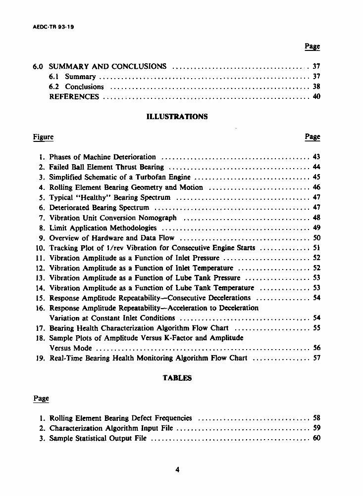
6.0 SUMMARY AND CONCLUSIONS ...................................... 37

6.1 Sum m ary .......................................................... 376.2 Conclusions ....................................................... 38REFERENCES ......................................................... 40

ILLUSTRATIONS

Figure Page

1. Phases of Machine Deterioration ......................................... 432. Failed Ball Element Thrust Bearing ....................................... 443. Simplified Schematic of a Turbofan Engine ................................ 454. Rolling Element Bearing Geometry and Motion ............................ 465. Typical "Healthy" Bearing Spectrum ..................................... 476. Deteriorated Bearing Spectrum ........................................... 477. Vibration Unit Conversion Nomograph ................................... 48

8. Limit Application Methodologies ......................................... 499. Overview of Hardware and Data Flow .................................... 50

10. Tracking Plot of 1/rev Vibration for Consecutive Engine Starts .............. 5111. Vibration Amplitude as a Function of Inlet Pressure ........................ 5212. Vibration Amplitude as a Function of Inlet Temperature .................... 5213. Vibration Amplitude as a Function of Lube Tank Pressure .................. 5314. Vibration Amplitude as a Function of Lube Tank Temperature .............. 5315. Response Amplitude Repeatability-Consecutive Decelerations ............... 5416. Response Amplitude Repeatability-Acceleration to Deceleration

Variation at Constant Inlet Conditions .................................... 5417. Bearing Health Characterization Algorithm Flow Chart ..................... 5518. Sample Plots of Amplitude Versus K-Factor and Amplitude

Versus M ode ........................................................... 56

19. Real-Time Bearing Health Monitoring Algorithm Flow Chart ................ 57

TABLES

Page

1. Rolling Element Bearing Defect Frequencies ............................... 582. Characterization Algorithm Input File ..................................... 59

3. Sample Statistical Output File ............................................ 60

4

AEDC-TR-93-19

Table Page

4. Sample Histogram ................................................. 615. Fault Frequency Combinations and Diagnoses ............................. 616. Health Monitoring Algorithm Input File .................................. 627. CADDMAS Capabilites Versus HEMOS Requirements ...................... 64

NOM ENCLATURE .................................................... 65

5

AEDC-TR-93-19

1.0 INTRODUCTION

1.1 HISTORICAL BACKGROUND

By definition, monitoring is an act of extracting information from a system by observing

instruments (sensing). Hence, online vibration monitoring consists of continuously acquiringvibration signals and using those reduced data as near real-time indicators of machine health.

Figure 1 shows the three phases of a typical machinery deterioration versus run-time curve.Phase I is the run-in time; Phase II is the normal operation period; and Phase III is the failure

development period. Early failure prediction sought by the online vibration monitoring systemis designated by state "A" on the figure (Ref. 1).

The primary applications of online vibration monitoring programs have been in the paper,power, and chemical industries where relatively constant load operation of rotating machinerylends itself to near real-time monitoring. Continuous condition monitoring is a maintenancetool in these industries which allows predictive maintenance programs which are based onearly warning. Here, the motive is to avoid unplanned shutdowns and minimize the cost oflost production (Ref. 1).

Importantly, detection of rolling element (ball or roller) bearing component faults, throughvibration diagnostic techniques, has proven to be among the most reliable analysis tools fordeducing mechanical faults in the relatively low-speed pumps, compressors, turbines, motors,etc. on which these industries rely (Refs. 2 and 3). Application of the principles of bearingfault diagnostics to high-speed turbomachinery such as aircraft turbine engines is, however,in its relative infancy (Ref. 4).

Implanted fault testing and post-mortem vibration analyses of bearing failures have shownthat bearing fault diagnostics may also be successfully applied in aircraft turbine engines(Ref. 5). In some cases, post-failure analysis has uncovered indications of significant bearingfaults minutes and even hours prior to catastrophic failure (Ref. 6). A dramatic exampleincludes failure analysis of the bearing, shown in Fig. 2, in which the cracked cage, race,and rolling element faults were correctly diagnosed prior to engine teardown.

If the analyst's thought processes can be automated, then future bearing faults can bedetected through online monitoring before a catastrophic failure manifests. The primary goalof the research reported herein is to develop such an algorithm.

Efforts involving determination of feasibility and preliminary requirements for anautomated vibration-based online health monitoring system were conducted in S/T 147 projectBC69EJ, Turbine Engine Durability. In FY93, the research effort was transferred to S/T

7

AEOC-TR-93-19

130 with the goal of developing the AEDC vibration-based Health Monitoring System(HEMOS) as an augmentation to the Computer Assisted Dynamic Data Monitoring and

Analysis System (CADDMAS), project 0088. Efforts in FY93 focused on algorithm

development for characterization and health monitoring based on bearing vibration. The

ultimate goal of the HEMOS effort is to incorporate case, gear box, and frame-mountedvibration sensors, along with transient digital data, to survey overall health of the turbine

engine test articles on test at AEDC.

1.2 STATEMENT OF PROBLEM

Applied to machinery which operates at steady-state conditions for long periods, bearing

fault diagnosis is a reliable, well-understood technique. In this case, developing faults tend

to appear as changes to the vibratory response characteristics of the machine. The task ofdeciphering developing faults through vibration monitoring becomes much more difficult,

however, when multistate variable operating turbomachines are involved. Aircraft engines

by nature are extremely transient machines. Requirements to operate over a wide range ofaltitudes and flight velocities translate into an extensive matrix of inlet conditions (i.e., pressure,temperature, density, etc.). Since vibratory responses can vary significantly with one or more

of these factors, a huge array of data may be required to define a baseline vibration signaturefor a specific engine model. A bearing health characterization algorithm is developed in Section5.0 to accommodate this task in an offline mode.

The body of knowledge concerning bearing vibrations and related information has been

investigated through an exhaustive literature survey. Two shortfalls which have been identified

in the literature include:

1. Most published work is devoted to a particular bearing application on a specific

machine.

2. Little work has been done to analyze the influence of bearing operatingparameters on the vibratory environment.

This research effort addresses each of these shortfalls. First, the algorithm is adaptable

by means of an input file to function for a variety of rolling element ball bearings in a numberof different turbomachine applications. Second, influence of the primary bearing operatingparameters on the bearing housing vibratory environment is analyzed. Identified trends are

reported herein.

8

AEDC-TR-93-19

1.3 ENGINE OVERVIEW

Since much of the material presented is devoted to bearing vibrations in aircraft turbine

engines, an overview of engine design and operation is presented. Many of the jet engines

currently in use are of the turbofan design shown in simplified schematic form in Fig. 3.

These machines employ dual, concentric rotors. A low-pressure compressor or fan feeds

compressed air to a high-pressure compressor (HPC) and a bypass duct. Air entering theHPC is further compressed before entering a combustion chamber (COMB) where fuel isinjected, atomization transpires, and controlled combustion takes place. The hot exhaust

gases are then expanded through a single or multistage high-pressure turbine (HPT). Furtherexpansion then takes place through a low-pressure turbine (LPT) before mixing of the exhaustgases with the bypass air. The total mass flow is then exhausted through the tailpipe.

The HPC and HPT are connected via a shaft, and the combined assembly rotates at aspeed (designated high rotor speed, NH) determined by design conditions and power setting.The high rotor assembly is generally supported by a forward-mounted ball element thrust

bearing and an aft-mounted roller element radial bearing.

The fan and LPT are connected by a second shaft rotating at low rotor speed, NL, and

similarly supported by two additional bearings. The low rotor shaft feeds through the highrotor shaft, and relative motion between the two shafts is constrained by an intershaft

fifth bearing.

Due to space constraints within the engines, bearing vibration instrumentation is normallylimited to radially oriented, housing-mounted accelerometers or velocity pickups. Rarely,

proximity probes are employed through a housing penetration port to measure shaftdisplacement directly. Axially oriented vibration sensors are primarily used only on the engineouter case near the support frames since the concentric rotors inhibit access to the internal

bearings. Also due to limited access, the intershaft bearing is seldom instrumented.

1.4 LIMITATIONS OF THE RESEARCH

The bearing health algorithm was developed for application to rolling element bearingsin the diameter times running speed, DN, classification range from 1.0 x 106 to 1.8 x 106.

This classification generally encompasses most high-speed turbine engine ball element thrustand roller element radial support bearings. The algorithm is generic in nature, however, andcould be applicable to much higher DN class bearings. Though automation of the algorithm

9

AEDC-TR-93-19

is outside the scope of this report, current plans for FY94 HEMOS work include automationof both the characterization and health monitoring algorithms. Preliminary vibrationcharacterization of a single engine family and implementation of a prototype HEMOS arealso planned.

Due to the widely varied conditions to which jet engines are subjected, analysis of vibrationdata to determine the effects of operating parameters was limited to data from a single verticallymounted bearing accelerometer operating over a range of speeds from idle to maximum power.Data from 21 different flight conditions were analyzed. Though the survey of vibration

data was limited, several important conclusions may be drawn from the results (seeSection 4.0).

The effort expended on the manual analysis points to the necessity for automating thisprocess. A methodology for such automation is presented in Section 5.0 and will be automated

in subsequent research.

It should also be noted that the algorithms developed herein rely on Fast Fourier

Transformation (FFT) of vibration data. This technique is not adequate to capture bearing

faults which occur during true transient conditions such as extremely high acceleration anddeceleration rate maneuvers in turbine engines. Wavelet decomposition has been studied asa means of identification of bearing faults during such maneuvers (Ref. 7). The healthmonitoring algorithm should, however, identify fault symptoms during quasi-equilibrium

conditions. Provided sudden, catastrophic failure does not occur during extreme throttle rateexcursions, the health monitoring algorithm should be able to detect bearing faults once themachine has returned to a quasi-equilibrium state.

1.5 APPROACH

The research reported herein consisted of several phases. First, the bearing fault frequencyequations were developed. Second, data analysis techniques for characterizing the vibratoryresponses measured at the bearing housing were designed. Next, an investigation of the effects

of various machine operating parameters on the vibratory responses was conducted.Finally, a statistical approach was employed to ascertain bearing health criteria, and thesecriteria were incorporated into a functional algorithm which can be used in an automatedmonitoring capacity.

Phase I of the study developed the formulae for the bearing fault frequencies usingkinematic analysis. Figure 4 illustrates the geometry and motion of a generic rolling element

bearing (Ref. 8). The bearing fault frequency calculations are included in Table I (Ref. 2).

10

AEOC-TR-93-19

The fault frequencies, which include the fundamental train frequency (FTF), the ball spinfrequency (BSF), ball passing frequency-outer race (BPFO), and the ball passing frequency-inner race (BPFI), are presented in Section 2.0.

Phase 2 of the research examined historical vibration data to determine the analysistechniques required for development of health criteria. Research activities reported include:(1) assessment of the most viable physical quantity of vibration (displacement, velocity, oracceleration) on which to base the algorithm, (2) determination of adequate means of datareduction and presentation (i.e., time domain, spectral plots, engine-order tracking plots,etc.), (3) results of an investigation to determine the primary bearing responses and theexcitation source for each, and (4) development of two distinct modes of operation for thealgorithm, including an evaluation of various data windows (i.e., start-up, coast-down, part-power, and maximum rotor speed) for incorporation into a data trending segment of thehealth monitoring algorithm.

Phase 3 of the study examined the influence of various operating parameters on the bearingvibratory response characteristics. Parameters which were found to have primary or secondaryeffects on the vibratory environment include operating shaft speeds, engine inlet pressure,engine inlet temperature, bearing lubrication pressure, and bearing lubrication temperature.Several important conclusions were drawn from this phase.

The final phase (Phase 4) incorporated a statistical approach to determine the relativehealth of lubricated rolling element bearings in high-speed turbomachinery for incorporationinto the health monitoring algorithm. Figure 5 depicts a spectral response from anaccelerometer mounted on a "healthy" bearing. The machine is operating at 6000 rpm (100Hz). A once per revolution, 1/rev, response due to residual rotor unbalance is always present,as shown in the figure. Figure 6 5hows a vibratory spectrum indicative of a deteriorated bearing.Presence of the FTF and modulation of running speed harmonics by the FTF usually indicatea worn or cracked bearing cage. Similar frequencies were evident in the spectra leading upto the bearing failure illustrated in Fig. 2. Other bearing faults can be deduced dependingon the combinations of fault frequencies present (see Section 3.0). This phase of researchdeveloped an algorithm to statistically band the various vibratory response amplitudes andfrequencies in an offline mode.

2.0 ROLLING ELEMENT BEARING FAULT FREQUENCIES

In this section the bearing subcomponents are introduced, and the rolling motion withina bearing is discussed. The fundamental bearing fault frequencies are then developed throughkinematic analysis of the rolling motion.

11

AEDC-TR-93-19

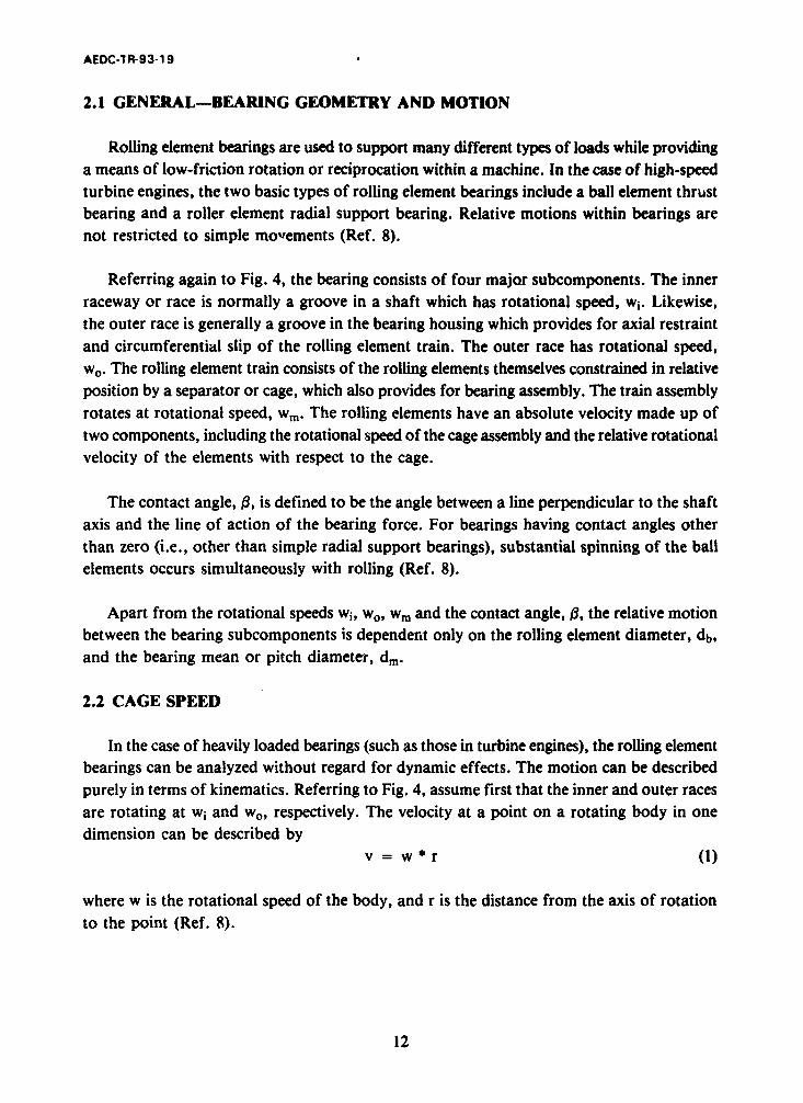
2.1 GENERAL-BEARING GEOMETRY AND MOTION

Rolling element bearings are used to support many different types of loads while providinga means of low-friction rotation or reciprocation within a machine. In the case of high-speedturbine engines, the two basic types of rolling element bearings include a ball element thrustbearing and a roller element radial support bearing. Relative motions within bearings arenot restricted to simple movements (Ref. 8).

Referring again to Fig. 4, the bearing consists of four major subcomponents. The innerraceway or race is normally a groove in a shaft which has rotational speed, wi. Likewise,the outer race is generally a groove in the bearing housing which provides for axial restraintand circumferential slip of the rolling element train. The outer race has rotational speed,wo. The rolling element train consists of the rolling elements themselves constrained in relativeposition by a separator or cage, which also provides for bearing assembly. The train assemblyrotates at rotational speed, win. The rolling elements have an absolute velocity made up oftwo components, including the rotational speed of the cage assembly and the relative rotationalvelocity of the elements with respect to the cage.

The contact angle, 0, is defined to be the angle between a line perpendicular to the shaftaxis and the line of action of the bearing force. For bearings having contact angles otherthan zero (i.e., other than simple radial support bearings), substantial spinning of the ballelements occurs simultaneously with rolling (Ref. 8).

Apart from the rotational speeds wi, wo, wm and the contact angle, 1, the relative motion

between the bearing subcomponents is dependent only on the rolling element diameter, db,

and the bearing mean or pitch diameter, dm.

2.2 CAGE SPEED

In the case of heavily loaded bearings (such as those in turbine engines), the rolling elementbearings can be analyzed without regard for dynamic effects. The motion can be describedpurely in terms of kinematics. Referring to Fig. 4, assume first that the inner and outer racesare rotating at wi and w., respectively. The velocity at a point on a rotating body in onedimension can be described by

v = w*r (1)

where w is the rotational speed of the body, and r is the distance from the axis of rotation

to the point (Ref. 8).

12

AEDC-TR-93-19

In the case of aircraft turbine engines, bearing vibration sensors (whether accelerometers,velocity pickups, or proximity probes) are oriented to pick up the radial component ofvibration. The equations are, therefore, developed in terms of the radial components ofvibration to be measured by these sensors. The radial velocity component at the inner raceand ball element contact point will be

vi = wi *ri

vi = 1/2 * * di

vi = ½ * wi * (dm - dbCOSt3) (2)

where ri is the distance from the shaft center to the inner race surface. The velocity at theouter race contact point is

Vo = WO * o

Vo = //z * W do

Vo = /2 * wo * (din + dbCOS 3) (3)

where ro is the distance from the shaft center to the outer race surface. Introducing,

/A = (db/dm) * cos 0 (4)

and multiplying Eqs. (2) and (3) by I/dm, respectively,

vi = ½2 *wi*dm(1 - it) (5)

Vo = ½ * w. d, (I + A•) (6)

Assuming no relative slip, the velocity of the rolling element train may be taken as the

mean of the inner and outer race velocities, vm, such that

Vm = 1 * (vi + vo) or,

Vm = /4 *dm * {wi 0 - /U) + wo 0 + 01) (7)

But,

13

AEDC-TR-93-19

Vm = 1/2 *WM *dm (8)

Substituting Eq. (8) into Eq. (7) and solving for wm yields

Wm = V2 {wi (1 ) + Wo ( + ) (9)

which gives an expression for the cage rotational speed in terms of the inner and outer racespeeds and bearing geometry. Recognizing that

w = 21rf, and substituting into Eq. (9) yields

fm = '/2 * {f. (1 - A) + fo (1 + #)} (10)

which establishes the cage frequency, fro, in cps with respect to a fixed reference frame (i.e.,the vibration sensor).

2.3 ROLLING ELEMENT SPEED

To determine the rotational speed of the ball, Wb, we first introduce the angular speedof the cage relative to the inner race:

Wmi = wm - Wi (11)

Assuming no slip, the ball velocity, Vb, is identical to the velocity of the inner raceway atthe point of contact. That is,

Vb = vmi at the point of contact. (12)But,

Vb = Wb * rb = V2 * Wb * db, and (13)

Vmi ---Wmi *rmi = V2 * Wmi * d m (1 -/)(14)

Substituting Eqs. (13) and (14) into Eq. (12) gives

S* Wb * db = V2 * wmi * dm (I -t) or,

Wb = (dm/db) * Wmi (1 - 1t) (15)

14

AEDC-TR-93-19

Substituting Eq. (11) into Eq. (15) and again invoking

w = 2rf

fb = (dm/db) * fm - f) * (I - A) (16)

Substituting Eq. (10) into Eq. (16) for fm yields

fb = (dm/db)*(I - A)* {1{f2(J - A) + fo(l + A)} - f

fb = (dm/db) * (I - A)* {P/2fi - A - VafiJU + V2/fo( + 0)}

fb = (dm/db) * (1 - A)* {I/2fo( + 1) - ½fi(l + 0I)

fb = ½ * (dm/db)* (1 - L)* (1 + A)* (o - fi) (17)

Here, the frequency associated with the rolling element velocity relative to the cage has

been determined. This is the frequency which may be detected by a vibration sensor in the

event of a rolling element fault (Ref. 8).

2.4 SPECIAL APPLICATION

In the special case of a jet engine, most bearings have a stationary outer race and a rotating

inner race. Thus, fo = 0 and Eqs. (10) and (17), respectively, reduce to

fm = ½fi(l - ut), and (18)

fb = -- Y(dm/db) * (0 - At) * (I + A) * fA (19)

The minus sign in Eq. (19) simply refers to the fact that the radial ball spin is opposite

in direction relative to the cage rotation. Obviously, the vibration sensor will detect only

the absolute frequency, or

fb = V2(dm/db) * (1 - 14) * (I + s)fi (20)

For a healthy bearing with proper clearance fit and no macroscopic defects, the vibration

introduced by the cage and rolling elements contributes no significant amplitude, and vibration

at fm and fb is masked by random vibration energy (i.e., in the noise band of the spectrum).

The bearing fault frequencies will now be developed for the special case of a stationary outer

race and rotating inner race as found in the turbine engines tested at the AEDC.

15

AEDC-TR-93-19

2.5 FUNDAMENTAL TRAIN FREQUENCY (FIT)

If the bearing is too loose or the cage is worn or cracked, discrete vibration amplitudesat fm (FTF) and its harmonics may appear. If the defect is severe enough, the harmonicsof running speed (i.e., multiples of fj are modulated by FTF, and ± sidebands of FTF willappear in the spectrum (cf. Fig. 6). So, the first bearing fault frequency has been derivedfor the special cabe of stationary outer race and rotating inner race.

FTF =fm = Vfi(l - it) (21)

2.6 BALL PASS FREQUENCY-OUTER RACE (BPFO)

If there is a significant defect on the outer (stationary) race, then each rolling elementproduces an impact vibration as it rolls over the defect. The frequency which is generatedby this phenomenon is related to the cage motion relative to a fixed reference frame. Thevibration measured by the sensor will manifest at

BPFO = n * FTF = (n/2)fi(l - it) (22)

where n is the number of rolling elements.

2.7 BALL PASS FREQUENCY-INNER RACE (BPFI)

If there is a defect on the inner (rotating) raceway, then a spike caused by the impactingof each rolling element as it contacts the defect again manifests as vibration. Note that thefrequency of vibration in the fixed reference frame is due to the relative rotational speedof the inner race and the cage assembly such that

n * wrwr = n * (wi -- W.) (23)

which reduces to

BPFI = n * frued

BPFI = n * (fi - fin)

BPFI = n * Vi - FTF) (24)

16

AEDC-TR-93-1 9

Substitution for FTF gives

BPFI = fi- 'Afi(l -)= V2fi + ½fip

BPFI = 112fi(l + 1&) (25)

2.8 BALL SPIN FREQUENCY (BSF)

Finally, a single defect on a rolling element generates a measurable vibration at the relativespin frequency of the ball relative to the cage. Or, from Eq. (20),

BSF = fb = ½(dm/db) * (I - #&) * (I + it) * i

BSF = V2(dm/db) * j * (1 - #t2) (26)

with stationary outer race.

For the case of multiple rolling element defects, the frequency generated is simply amultiple, m * BSF, where m is the number of defects.

2.9 BEARING FAULT DIAGNOSIS

In the preceding sections, the bearing fault frequencies have been developed through anunderstanding of the relative motion between the bearing subcomponents and how they relateto a fixed observer (i.e., a radially mounted vibration sensor). A survey of the axial vibrationis omitted since, in practical jet engine applications, clearances do not permit instrumentationof bearing housings mounted in an axial orientation. AEDC experience reveals that mostbearing health-threatening defects may be detected through monitoring of the radial

vibration alone.

Healthy bearings, in general, do not exhibit significant amplitudes of vibration at thebearing frequencies. When a defect is present, however, discrete responses can usually bedetected at one or more fault frequencies. Initial presence of a measurable amplitude at afault frequency abc.'e the spectral noise floor i analogous to detection of state "A" in Fig.1. An experienced vibration analyst can usually track progression of worsening defects throughchanges in amplitudes and spc-tral content. Planned research activities will attempt tocharacterize this progression for incorporation into a health monitoring algorithm.

17

AEDC-TR-93-19

For the effort to date, however, the primary goal of the bearing health algorithm is toidentify potential life-threatening defects as they initiate. If state "A" can be identified, thenonline operators may be able to take precautionary measures based on algorithm alarms.

3.0 DATA ANALYSIS TECHNIQUES

This section develops the data analysis techniques required to adequately characterizebearing vibration and implement a health monitoring algorithm. First, the quantities ofvibration, (displacement, velocity, and acceleration) are discussed, and their interrelationshipsare examined. Second, data presentation alternatives are introduced. Third, the primary bearingresponses are investigated, and limit application methodologies are discussed. Finally, amonitoring system overview is presented, and the continuous and trend modes are explained.

3.1 PHYSICAL QUANTITIES OF VIBRATION

In the realm of vibration analysis, questions often arise concerning the most usefulmeasured physical quantity for a specific application. Before looking more closely at variousapplications, the relationships between the physical quantities of vibration are examined.These quantities include displacement, velocity, and acceleration.

R. F. White makes a strong case for defining limits in terms of peak velocity (Ref. 9).He argues that velocity is proportional to the energy of vibration and is independent offrequency in the energy equation. He states that limits may be defined over a broader frequencyrange with less maximum-to-minimum deviation than displacement and acceleration limits.A development and analysis of the equations involved, however, leads to the conclusion thatvelocity alone is not satisfactory for a bearing health monitoring application.

Assuming steady-state sinusoidal motion of a body, the time-dependent displacement,D, is described as

D = B sin (wt) (27)

where the peak displacement, B, is in inches; the angular velocity, w = 21rf, is in rps; andfrequency, f, is in cps or Hz. The velocity, v, may be taken as the derivative of displacementsuch that

v = d/dt(D) = Bw cos (wt) = 21rfB cos (wt);

v = 21rfB sin (wt + 90) (28)

18

AEDC-TR-93-19

where the velocity is in in./sec (or ips). The acceleration, a, is the derivative of velocity such that

a = d/dt(V) = - Bw2 sin (wt)

a = (2ih)2B sin (wt + 180) (29)

where acceleration is expressed in in./sec2.

Recognizing that the sinusoidal phase shifts in Eqs. (27), (28), and (29) simply refer tothe fact that velocity leads displacement by 90 deg and acceleration leads displacement by

180 deg, examine the relationships between the peak values of displacement, velocity,

and acceleration.

Setting wt = 0 deg in Eq. (28) yields the relationship between peak velocity and

peak displacement:v = 21-fB or B = v / (21rf) (30)

where v is now peak velocity (ips pk).

Setting wt = 270 deg in Eq. (29) yields the relationship between peak acceleration and

peak displacement:

a = (2,rj)2B or B = a / (21'f)2 (31)

where a is now in in./sec2 peak.

Equating the right halves of Eqs. (30) and (31) yields the relationship between peak

acceleration and peak velocity:

a = 2-fv or v = a / 2wf (32)

Now, introduce I mil = 0.001 in., and I g = 386.087 in./sec2 at sea level. These

units of displacement and acceleration, respectively, are much friendlier for application tovibration theory.

Further, define d = 2B to be the peak-to-peak displacement of the body. On proper

substitution and conversion, the relationships in Eqs. (30), (31), and (32), respectively, become:

d = 318.3 * (v/I) or v = df/318.3, (33)

19

AEDC-TR-93- 19

a = / 139.85) * d or d = (139.85 /.z * a, (34)

a = V v) / 61.43 or v = 61.43 * a /f (35)

By looking at these simplified equations, we get an intuitive feel for which units (and

thereby which types of sensors) are most useful for different applications. Note that mostamplitudes of vibration in high-speed turbomachinery range from 0 to 10 mils peak to peak

(pk-pk), 0 to 0.5 ips peak, and 0 to 20 g's peak.

In Eq. (33), note that displacement and velocity become equal at f = 318.3 Hz, suggesting

that as frequency increases far above 318 Hz, displacement measurements grow smaller andsmaller for constant velocity. Atf m 1600 Hz, measured displacement is less than I percentof -the maximum full-scale range of expected vibration. As such, most sensors are unableto resolve discrete displacement components at higher frequencies. Conversely, vibrationsat much lower frequencies (f s 2 Hz) render the velocity spectrum nearly useless, anddisplacement amplitude resolution is far better.

Similarly, Eq. (34) shows that acceleration and displacement become equivalent atf - 140 Hz. Much smaller displacements become significant at higher frequencies for constant

acceleration (due to the f2 term), and units of acceleration are preferable at frequencies above800 Hz. Equation (35) indicates that velocity and acceleration become equivalent at - 61Hz. At frequencies greater than approximately 1200 Hz, vibration responses indicative ofa rolling element fault are in the noise band of the velocity spectrum, but discrete peaksindicative of race faults are discernible in the acceleration spectrum.

To examine the effects of frequency on amplitude of displacement, velocity, andacceleration more closely, examine the nomograph in Fig. 7 and consider the following"example. Point P in the figure is plotted at a vibratory frequency of 8 cps or Hz. Displacementamplitude is 4 mils pk-pk; velocity amplitude is 0.09 ips pk; and acceleration amplitude is

0.01 g's pk. By generally accepted guidelines, 4 mils pk-pk is relatively alarming; 0.09 ipspk is fairly benign; and 0.01 g's pk is of little concern. The analyst must discern the excitationsource for the response and determine its potential impact to the rotating machine. Importantly,a 4 mils pk-pk displacement response at the FTF identifies a bearing nearing catastrophicfailure, whereas an acceleration of only 0.01 g's pk likely lies within the noise band of the data.

Point Q in Fig. 7 illustrates a converse situation. At 10,000 cps, displacement amplitude

is 0.002 mils pk-pk; velocity amplitude is 0.065 ips pk; and acceleration amplitude is 10 g's

pk. In this case, velocity and displacement amplitudes warrant no particular concern, whereasacceleration energy is at the danger level. Frequency has an obvious effect on the amplitudes

20

AEDC-TR-93-19

of response, and the analyst must take into account the physical quantity of vibration

(displacement, velocity, or acceleration) before concluding relative machine health.

Since the class of high-speed turbomachinery investigated herein has bearing fault

frequencies which vary from approximately 30 Hz to 2000 Hz, it seems prudent to adapt

the algorithm to take advantage of all vibration quantities: displacement, velocity, and

acceleration.

Experience in analyzing vibration data from turbine engine bearings suggests the following

frequency ranges for the physical quantities of vibration are an acceptable guideline:

displacement - 0 to 500 Hz,

velocity - 200 to 1200 Hz, and

acceleration - 800 to 10,000 Hz.

In addition to the theoretical development and inherent advantages, there is a very good

practical reason for taking this approach. All jet engine manufacturers do not use similar

vibration sensors. Proximity probes measuring displacement, velocimeters measuring velocity,

and accelerometers measuring acceleration are all used in some applications for determining

the engine vibratory characteristics.

3.2 DATA PRESENTATION ALTERNATIVES

The AEDC vibration-based HEMOS, when fully developed, should be capable of providing

all usual vibration data presentation formats including (but not limited to): spectra, trendingplots, engine-order tracking plots, waterfall plots, Campbell diagrams, orbits, Bode' plots,

Nyquist plots, tables, alarm synopses, etc. (Ref. 6). For primary health monitoring purposes,

however, modified spectra of vibratory amplitude versus K-Factor and amplitude versus

vibratory mode are used. This approach is explained in detail and justified later in this section.

3.3 PRIMARY BEARING VIBRATORY RESPONSES

To ascertain the most likely responses of bearings to vibration stimuli in jet engines, recallthe engine description introduced in Section 1.3 and examine the purpose of the bearings.Rolling element bearings in these high-speed turbomachines are required to provide smoothoperation of the rotor shafts and to transfer unwanted energy in the form of vibration out

of the machine through the support frames.

21

AEDC-TR-93-19

Based on the overall assembly, some primary response frequencies can be surmised. Sinceall rotating assemblies have some residual unbalance due to manufacturing tolerances, material

flaws, etc., each of the bearings responds to a 1/rev excitation, and this response is measured

by a sensor due to passing of the rotor's heavy spot (attributed to residual mass unbalance,

i.e., eccentricity). The frequency of vibration occurs at rpm/60. Since the two rotors rotate

at different speeds, it can be safely assumed that the high rotor support bearings will primarily

respond at 1/rev of the high rotor shaft (IX NH), and the low rotor bearings will respond

at IX NL. Depending on the energy of vibration and shaft alignment within the bearings,

harmonics of the IX responses may also occur at 2X, 3X, etc.

Since a path of vibration transmissability between the two shafts exists in the form of

the intershaft bearing, the thrust and radial support bearings of the low rotor will likely respond

(to a lesser degree) to the IX NH stimulus, and the high rotor bearings will respond (to a

lesser degree) to the IX NL excitation.

The above responses are deemed to be normal and provided they are within acceptable

limits, pose no threat to the turbomachine hardware. There are other responses, however,

which indicate potential health hazards to the engine (R. L. Eshelman, "Machine Diagnostics,"

Vibration Institute: Machinery Vibration Analysis 1, Course Notes, Nashville, TN, November

17-20, 1987). Such responses include:

I. Extreme IX NH or NL due to a bowed or bent rotor,

2. Significant 2X NH or NL attributable to a shaft which is severely misaligned

in its bearings,

3. Subsynchronous vibration at 0.4X to 0.48X NH or NL indicative of an oil whirl

phenomenon,

4. Any of the bearing fault frequencies described in Section 2.0 which betray the

presence of localized defects within the bearing,

5. Vibration at 0.5X NH or NL and due to seal rubs, blade tip rubs, or coupling

looseness,

6. Extreme vibration at 0.25X or 0.33X and harmonics due to a subsynchronousresonance (oil whip),

7. Sum and difference (beat) frequencies such as (NH - NL) or (NH + NL)

which excite damaging hardware resonances, and

22

AEDC-TR-93-19

8. Rarely, vibration at a known blade-passing frequency which excites a framestrut aeromechanical resonance (Ref. 6).

Now that an understanding of the hardware assembly and the primary expected bearingresponse frequencies has been developed, an important insight into the duties which can befalla bearing health monitoring algorithm is gained. An investigation of two limit application

methodologies follows.

3.4 METHODOLOGIES FOR LIMIT APPLICATION

Because of the transient nature of aircraft engines, a methodology was needed for

comparison of vibratory responses to established limits. To investigate further, a typicalturbofan engine with a low rotor operating speed regime of 3000 to 6000 rpm was considered(Fig. 8 and Ref. 6). At 3000 rpm (Fig. 8A, top), a IX response of 2 mils pk-pk at 50 Hz(3000 rpm) and a 2X response of I mil pk-pk at 100 Hz would be indicative of a relativelyrough running rotor (2 mils IX at idle) with bearings that are poorly aligned to the shaft.

When accelerated to 6000 rpm (Fig. 8A, lower), a IX response of 2 mils pk-pk occurs

at 100 Hz (6000 rpm), and no significant 2X component of vibration was noted. This responsecharacteristic represents a healthy engine which is operating well within the vibration limitsof most manufacturers.

In the first case, a 100-Hz response of 1 mil pk-pk was interpreted as a fault (bearing

misalignment); in the second case, a 100-Hz response of 2 mils pk-pk was deemed to be normal.

Consequently, the limit application methodology in a turbine engine vibration monitoringsystem must be able to recognize the various responses in the spectrum and apply the

appropriate limits, suggesting a sliding mask limit application technique where a limit envelope

(or mask) must change with changing speeds. Theoretically, a different limit mask exists forevery combination of low and high rotor speeds, and an expert system is required tocontinuously identify the significant spectral responses and apply the appropriate limits. Thelimit mask must slide to the right in the frequency domain as the engine is accelerated from3000 rpm (Fig. 8A, top) to 6000 rpm (Fig. 8A, lower).

By employing the K-Factor approach to the limit application illustrated in Fig. 8B, theproblem becomes greatly simplified. The K-Factor approach draws on the fact that all rotor

dynamic responses are related to rotor speed in an integral or nonintegral manner, such that

f = K-Factor * N / 60or,

23

AEDC-TR-93-19

K-Factor = f * 60 / N

where N is high or low rotor speed, NH or NL, and K-Factor is a constant related to geometry

or phenomena.

For integral vibrations, the K-Factor is simply an integer multiple of engine speed. For

nonintegral vibrations, K-Factor is a mixed fractional number (i.e., K-Factor -, 0.47 forvibration due to oil whirl phenomenon). These responses are easily computed, so if the nominalresponse range for a given engine family can be characterized in terms of amplitude versusK-Factor, then the bearing algorithm can be programmed to interrogate for potential problems

using a single limit mask and avoid the huge development task associated with a sliding mask

(Ref. 6).

The selection of the K-Factor approach to limit application is a potential means of avoidingone of the major pitfalls of automated health monitoring systems: false alarms. By separating

the vibratory responses associated with NiH and NL for each sensor's data stream, confusionover which responses are nonsynchronous (and thus potential fault indications) maybe avoided.

Yet another limit application is required due to the nature of modal vibration. In somecases (e.g., a bearing housing resonance), vibrations occur across the speed regime at nearconstant frequency. This form of vibration results in a smearing effect in the amplitude versusK-Factor spectrum. Therefore, the algorithms must take into account known modal responses,and alert and alarm limits must be established into a limit application methodology. Themeans by which this form of vibration is handled by the algorithms is discussed more fullyin Section 5.0.

3.5 MODES OF ALGORITHM OPERATION

To avoid confusion with vibratory modes of the engine components, the bearing healthmonitoring algorithm has two separate, parallel modes of operation. First, the continuous

mode of the algorithm acts as a watchdog for potential hardware faults as they initiate and

develop. The trend mode screens acquired data during special user-defined "windows" ofoperation to quantify overall rotor system degradation and potential faults which manifest,but may not exceed the limits imposed in the continuous mode of operation. An overviewof the hardware involved and the data flow is shown in Fig. 9 (Ref. 6).

In the continuous mode, acquired vibration and transient digital data are continually

merged and passed to a host computer system where the monitoring algorithm may be appliedto the processed data. The transient digital data include engine rotor speeds (NH and NL),

24

AEDC-TR-93-19

lube oil pressures and temperatures, and inlet conditions (altitude, Mach number, pressure,temperature, density, etc.). The continuous mode of the algorithm checks vibrations versusmanufacturer's specified limits and screens for potential rotor dynamic and bearing faults.If no potential problems are identified, the merged data remain in a circular file to beoverwritten. Should a potential problem be identified, however, an alarm system identifiesthe channel(s) in an overlimit condition, and the data from all channels are written to a filefor permanent storage. In the case of an alarm condition, the circular file data are also dumpedimmediately to permanent storage to provide a 20-min history of the engine conditions leading

up to a fault. A user interface is provided to: (1) input necessary information for the algorithmand (2) allow interaction for user interrogation of the permanent storage file. The continuousmode is operational whenever the engine is rotating (Ref. 6).

Before discussing the trend mode of algorithm operation, a practical example is requiredto examine the need for such a mode. On shutdown following a turbine engine test, a sealrub apparently took place along a rotor shaft. Localized heating occurred and resulted ina permanent set (bow) of the shaft. On start-up for the next test period, the engine acceleratedto idle speed without encroaching on a manufacturer-specified vibration limit. As the enginewas accelerated toward maximum power, however, extreme vibration was noted, and theengine was shutdown immediately. Unfortunately, significant damage occurred before theshutdown was ordered.

As shown in Fig. 10, post-event analysis indicated that a major shift in rotor critical speedof approximately 250 rpm and maximum attained amplitude had occurred between consecutivestarts of the engine. Through investigation of these data windows, it became obvious thata major shift in rotor dynamics had taken place. If a trend mode algorithm had been in place,the changes would have been recognized, and the hardware damage induced on engineacceleration toward maximum power may have been avoided.

The trend mode of the algorithm is invoked on use; demand to provide a historical datatrending capability during defined data windows. Potential windows may include enginestarts/shutdowns, 2-min accelerations and decelerations at health check flight conditions,baseline vibration data at maximum power, etc. Each of these windows is chosen to identifyshifts in rotor dynamic characteristics and to quantify engine deterioration in a further effortto identify state "A" (initiation of hardware faults) shown in Fig. 1. The trend data softwareshould compute statistical variations of current data with the historical database and generatea user-specified hardcopy comparison or CRT display for the vibration analyst(s). The trendmode allows visibility of pertinent trend information for all channels on user demand withoutinterrupting the flow of data through the continuous mode of the algorithm. A user interfaceis again necessary to specify input files, output format, and data window start/stop times(Ref. 6).

25

AEDC-TR-93-19

Detailed development of the continuous and trend modes of the red-time health monitoringalgorithm is presented in Section 5.5.

4.0 ANALYTICAL RESULTS

This section relates results of analysis conducted on response characteristics from a singlebearing housing-mounted accelerometer. First, the effects of bearing operating parameterson vibration characteristics are examined. Second, the repeatability of response amplitudesare compared during back-to-back decelerations and consecutive acceleration-to-decelerationthrottle movements at similar flight conditions. Finally, the necessity for automating theanalysis process is discussed.

4.1 BACKGROUND

Before an expert system can be programmed to identify abnormal conditions based onvibratory spectra, normal vibratory responses must first be characterized. Analysis wasconducted using reduced vibration data from a typical air-breathing turbofan engine. Thisengine was determined through analysis and teardown inspections to have no abnormal rotordynamic wear or degradation. The goal of this analysis included identifying the engineoperating parameters which have primary or secondary effects on the vibratory characteristicsof various engine components.

To limit the scope of effort, data from a single accelerometer were reduced and analyzedmanually. This vertically oriented sensor was chosen because it was the most responsiveaccelerometer to internal vibrations. For simplicity, the bearing-mounted accelerometer isdesignated B-VIB.

4.2 OPERATING PARAMETER EFFECTS ON VIBRATIONS

Preliminary investigation showed that several engine operating parameters influenced the

vibratory response characteristics measured. The primary response measured was always the1/rev signal generated by the residual unbalance of the high rotor (core) system. As noted

in Section 3.0, this was expected since the B-VIB sensor was mounted on the axial thrustbearing of the high rotor system. The function of this bearing is to restrain forward thrust-transmitting unbalance energy out of the engine in the form of vibration through the framestruts. Vibration amplitudes measured by B-VIB appeared to decrease with increasing inletpressure (Fig. 11), and the 1/rev response increased with increasing inlet temperature (Fig.12). These data were fitted using least squares curve-fit methods. Further investigation intothese trends, however, yielded an important result (Ref. 6).

26

AEDC-TR-93-19

At each of the two higher inlet pressure conditions shown in Fig. 11, the engine wasoperating at a control-specified pressure limit, and low rotor (fan) speed had been decreasedto maintain engine operation at this limit. Since the fan rotor and core rotor wereaerodynamically coupled, this resulted in a lower core speed as well. The result is a lowervibration amplitude measured at the bearing housing, because the residual mass unbalanceis rotating at a lower speed at higher inlet pressures (for identical power settings).

Data trends in Fig. 12 indicate increasing vibratory amplitude with increasing inlet

temperature for three different inlet pressures. Once again, these trends are actually relatedto NH. The fan speed schedule for most turbofan engine families is primarily a functionof inlet temperature subject to various pressure, temperature, and speed limitations. Fanspeed increases with increasing temperature (until limits are incurred), aerodynamically drivingcore speed higher as well.

Similar trends held for lube oil pressure and temperature, as shown in Figs. 13 and 14,respectively. Vibration amplitude increased with increasing lube tank pressure (Fig. 13), butfurther investigation revealed that this trend was also primarily related to speed. The constantvolume lube pump was driven by the core shaft through the power take-off (PTO) shaftand gearbox. Consequently, higher core speeds resulted in higher pump speeds and higherlube tank pressures. Vibrations once again increased with increasing core speed. Likewise,lube tank temperature had a secondary effect on vibration amplitude (Fig. 14). Increasingvibration with increasing lube temperature was again related to core speed through the gearbox(Ref. 6).

Although several parameters were found to have a secondary effect on vibrations measured

by B-VIB, the primary effect was always due to core rotor speed. In the absence of operation

at a critical speed (which is generally designed to be outside the engine operating regime),

the highest vibratory amplitudes are expected at the highest speeds and may be attributedto residual mass unbalance in the rotor. This is a significant conclusion, because if broadly

applicable, it greatly simplifies the approach necessary to monitor bearing health (Ref. 6).

If the normal range of vibratory amplitudes can be identified for each family of engines,

then it should be possible to screen for abnormalities based on 1/rev vibration and itsharmonics. Planned HEMOS efforts for FY 94 will attempt to characterize this normal range

of vibration statistically for a single engine family. Addition of a capability to calculate and

screen for the bearing fault frequencies will supplement the 1/rev monitoring, and a bearing

health monitoring scheme can thus be implemented via the bearing algorithm.

Engine manufacturers have well-developed limits for 1/rev NL and NH, and incorporation

of these limits into the monitoring methodology will be simple. Though more complicated,

27

AEDC-TR-93-19

expected resonant crossings for various components, caused by acoustic or wake shedding

excitation, may be computed. Parametric studies should be conducted to determine the range

of response magnitudes attributable to such resonances. For example, high vibratory stresses

in support frame struts sometimes induce vibratory responses measured at bearings. Provided

the algorithm is programmed to expect these resonances and associated increase in vibrations,false alarms will be kept to a minimum. Again, the difficulty lies in characterizing the expected

range of amplitudes for each resonant response, and further analysis is required.

4.3 RESPONSE AMPLITUDE REPEATABILITY

A representative plot of the variation in response amplitude versus frequency for the B-

VIB accelerometer is included as Fig. 15. For consecutive decelerations at similar inlet

conditions, B-VIB variation ranged from 0 to 8 percent for measured responses above the

noise floor. Similar variations were noted at other flight conditions as well (Ref. 6).

An investigation of acceleration/deceleration response amplitude variation was also

conducted (Fig. 16). Variations ranged from 0 to 22 percent for B-VIB. Due to significant

differences in bearing loads between acceleration and deceleration operation in some engine

families, further analyses are necessary to glean meaningful results for incorporation into

the algorithm (Ref. 6).

4.4 NECESSITY FOR AUTOMATION

The analysis results reported herein were a significant undertaking. Limiting the effort

to one data channel for a minimal number of engine data a-quisition events allowed certain

trends and conclusions to be drawn, but much is yet to be learned. Couple this level of

effort with the fact that output from one accelerometer at 21 flight conditions(accelerations/decelerations at each) was analyzed, and one begins to see the enormity of

analysis required to characterize the vibration responses over the flight map. The necessity

for automating the analysis process becomes apparent when it is realized that many turbofan

test engines are equipped with up to 12 bearing accelerometers, and many test programs

encompass 50 to 60 flight conditions (Ref. 6).

The bearing health characterization algorithm will first be applied to offline data. A

database of expected vibratory responses will be acquired for several test engine families.

Capabilities to statistically characterize the range of bearing vibratory responses were developedand are discussed in the next section.

28

AEDC-TR-93- 19

5.0 BEARING HEALTH CRITERIA AND MONITORING

As stated previously, the quest to identify faulty hardware components through automated

vibration monitoring must begin with the characterization of healthy hardware. The goals

of this section include: (1) development of a bearing health characterization algorithm,(2) examination of the role of operating environment on the vibration characteristics,

(3) examination of the significance of combinations of fault frequencies in fault diagnosis,

and (4) a discussion of the actual real-time bearing health monitoring algorithm and its decision-

making process.

5.1 BASELINE VIBRATION CONSIDERATIONS

Manufacturing and assembly tolerances can stack up to yield slightly different vibration

characteristics between even consecutive serial number engines in the same family. Slightvariations in bearing stiffness and alignment can influence the magnitude and speed at which

rotor dynamic resonances (critical speeds) occur. Further, balancing of individual rotor bladed

disks and subsequent stacking can yield differences in the amplitude of 1/rev vibration and

its harmonics for engines in the same family. Finally, control tolerances and mechanicallooseness in variable geometry can change mass flow and aerodynamic loading for similar

engines at like flight conditions and result in slightly different vibration characteristics. Forthese reasons, it is obvious that each family of air-breathing engines requires a statisticalbanding to identify the full regime of healthy vibration characteristics over the entire engine

operating envelope. The following algorithm was developed to provide such a characterization.

5.2 BEARING HEALTH CHARACTERIZATION ALGORITHM

Figure 17 illustrates the logic flow for the automated health characterization algorithm.

Although this discussion is limited to bearing-mounted vibration sensors, the algorithm may

be used to statistically characterize any engine-mounted vibration sensor. This algorithm isused in an offline mode to develop limits which may then be applied in the online health

monitoring algorithm. Referring to the numbered steps in Fig. 17, this section addresses each

division in the logic flow process.

Initially, data are read from an individual data channel. The data are first checked to

verify that incoming overall signal levels do not exceed the maximum voltage level obtainable

with the data conditioning equipment in use (Step 1). Generally, this is a maximum of

1.414 volts rms for our application. If a response level exceeds the maximum due to an

open, noisy channel, then the data are immediately omitted from consideration in the

characterization process.

29

AEDC-TR-93-19

Next, Fast Fourier Transformation (FFT) of the time domain data is accomplished forthe entire data event (Step 2). An event is typically a slow (-- 2 min) acceleration or decelerationor a health check point at steady-state operating conditions (i.e., speed, inlet conditionsconstant). The data are then temporarily stored as a succession of 1024 point ensembles.The usual digitization process using a Zonic model 6080 analog-to-digital conversion processorachieves about 2.5 ensembles per second of time domain data, though CADDMAS capabilitiesdiscussed later in this section should provide gapless data at 100 ensembles per second.

An input file is then read by the computer (Step 3). The input file includes a breakdown,by engine component, of all data channels. Each parameter is assigned a dynamic number,and each component includes one or more dynamic numbers. A switch, NSW, is includedto tell the program whether a component is more susceptible to high rotor or low rotorexcitation. For example, a No. 3 bearing accelerometer is more likely to respond primarilyto high rotor excitation since this bearing is the thrust bearing for the high rotor system.

Other information in the file includes known modal responses measured by each vibrationsensor. A housing resonance may exist, for instance, at approximately 750 Hz. Another keyinput includes frequency ranges indicative of line noise (e.g., 60 Hz TVA or 15 Hz cablewhip). An example input file is included as Table 2.

For each ensemble frequency, responses above a designated threshold are screened fornoise content as defined in the input file (Step 4). Any response occurring at a noise frequencyis automatically deleted from further interrogation.

K-Factors are then computed for each spectral response over a designated threshold level

according to the following hierarchy (Step 5):

NSW = NH, then Ki = f * 60 /NH

or, ifNSW = NL, then Ki = fi * 60 / NL

For simplicity, assume that NSW = NH. Each Ki is compared against multiples of highrotor speed (i.e., IX NH, 2X NH, etc.). If a match is found, then that response is categorizedaccording to its engine-order multiple, and all associated data (Ai, fi, Ki, NHi, NLi, etc.)stored in an array (Step 6). Once the data have been categorized at any point throughoutthe logic process, then they are omitted from further consideration. (In some engines, extremevibration may occur due to - combination of excitation sources such as IX NH = 2X NL.

Additional logic may be necessary for these special cases.) Unmatched responses at this pointhave new K-Factors computed based on low rotor speed, and the comparison process is

30

AEOC-TR-93-19

repeated in an effort to decipher responses associated with low rotor excitation. Matchedresponses are thereby categorized and stored. Unmatched responses continue through the logic.

Rotor dynamic responses related to rotor speed excitations are by far the most common.Further, any modal responses are likely to reach maxima at engine-order crossings.Consequently, the most important characterization information is gleaned through the K-Factor calculation and interrogation process.

Unmatched spectral responses after the K-Factor matching process are next interrogated

for modal frequency content based on the input file information (Step 7). If a response abovethe threshold falls into a frequency and speed regime defined in the input file, that responseis categorized, and pertinent data are once again stored. Unmatched responses are passed

on to the next phase of interrogation.

Beat (or sum and difference) frequency responses are fairly common in two-rotor systems.Based on AEDC vibration experience, primary beat responses occur at frequencies in Hz

of (NH - NL) / 60, (NH + NL) / 60, and/or (NH + NL) / 120. Step 8 in the algorithmsearches for beat frequency responses and stores pertinent information accordingly.

The goal of the execution is to categorize as many of the spectral responses possible foreach ensemble of data that is passed through the algorithm. Virtually all real-world dynamicsystems include random energy responses, however. Unmatched responses at this point in

the algorithm are classified as random, and each amplitude, frequency, Kj, NH, NL, etc.

is stored in a separate array (Step 9).

Step 10 in the algorithm computes and stores running average, maxima, minima, and

standard deviations for all K-Factors and modal frequencies, respectively. Once complete,the next ensemble of data is read in, and the process starts over again. When all ensembleshave been analyzed by the automated routine, the next data parameter is introduced

and processed.

After all parameters in a data set have been characterized, the algorithm produces threeoutput items which are key aides in determining appropriate limits for the actual real-timehealth monitoring algorithm (Step 11). These outputs include:

1. A table of statistical parameters for each vibration sensor characterized,

2. A histogram indicating the number of characterized responses as a percent ofmaximum amplitude, and

31

AEDC-TR-93-19

3. Plots of amplitude versus KNH, KNL, and Model.

Table 3 is an example of statistical output for a single parameter, and Table 4 illustratesa sample histogram.

Figure 18 illustrates the proposed combined plot format. In the amplitude versus K-Factorplot at left in Fig. 18, rotor dynamic related responses, which have been identified by thecharacterization algorithm, are shown. Minima, maxima, and averages are indicated for allidentified vibration responses above the specified threshold. The dashed line in this plotindicates a potential limit mask based on the data scatter and standard deviation data. Similarinformation for vibratory mode-related responses is shown at right in Fig. 18.

Once the characterization is complete for all sensors installed on a turbine engine,meaningful limits can be established for each family of engines for incorporation into thehealth monitoring algorithm discussed later in this section.

5.3 ROLE OF OPERATING ENVIRONMENT

In Section 3.0, it was concluded that the primary excitations of a single thrust bearingwere directly related to running speeds. Still, the turbine engine is a transient machine bynature, required to operate over a multitude of extremes. With the newly developed automatedcharacterization algorithm, further work can be accomplished in determining potentialinfluences of pressures, temperatures, variable vane angles, viscosity, density, etc. on therotor dynamic characteristics of the various machines.

Results of this further analysis can be incorporated into the algorithms as necessary tooptimize the health monitoring capability.

5.4 FAULT FREQUENCY COMBINATIONS

The characterization algorithm allows assessment of amplitude versus K-Factor andamplitude versus mode limits which may be incorporated into the health monitoring algorithm,as illustrated in Fig. 18. These limits should be specified to maximize the fault detectioncapability while minimizing incidence of false alarms. A healthy bearing should exhibit nofault frequency responses above the established noise floor (i.e., the established random energyof vibration at these frequencies). Appearance of significant amplitudes at K-Factors relatedto these frequencies indicates a developing fault.

R. L. Eshleman developed a table of fault frequency combinations and the associatedhardware faults, "Rolling Element Bearing Analysis," Vibration Institute: Machinery

32

AEDC-TR-93-19

Vibration Analysis 1, Course Notes, Nashville, TN, November 17-20. 1987. This informationis paraphrased in Table 5. Although the primary goal of the health monitoring algorithmis to alert engine operators of any potential hardware problem, the end-product monitoringsystem may well include a probable diagnosis based on the fault conditions identified.

5.5 REAL-TIME BEARING HEALTH MONITORING ALGORITHM

Figure 19 illustrates the logic flow process incorporated into the real-time bearing healthmonitoring algorithm. Similar to the characterization algorithm, each step in the decision-making process is labeled and discussed.

The initial step after data acquisition and conditioning is to apply a method of checkingfor spurious data (Step 1). This is likely to be a combination of checking for a saturatedchannel and interrogating the user-defined noise frequency bands (as accomplished in thecharacterization algorithm). Every effort is made to minimize false alarms, since such

occurrences degrade user confidence in the system.

The data are digitized and FFT-processed (Step 2). Care should be taken, however, topreserve a peak-to-peak voltage, Vpk-pk, as an indication of the overall vibration level fromeach vibration sensor.

As in the characterization algorithm, the health monitoring process requires that a user-specified engine data file be read (Step 3). This file includes information such as engine typeand model, engine serial number, thresholds, pertinent component geometries, accelerometerlocations, vibration parameter names and numbers, baseline vibration data from a historicaldatabase (discrete and overall), previous trending data windows, specific amplitude versusK-Factor and amplitude versus mode alert and alarm limits, and other pertinent information.This data file is used by both continuous and trend modes of the monitoring system andmust be read in at this point in the logic process. A sample input file is included as Table 6.

Overall vibration, 1/rev NL, and 1/rev NH responses are then screened versus specifiedmanufacturer's vibration limits (Step 4). The 1/rev NL and NH responses can be preservedusing digital filtering techniques. If a warning or alarm limit is surpassed, a yellow or redalarm is initiated and data from all channels downloaded into permanent file storage. Thisact does not stop the continued flow of data through the logic.

Assuming the online vibration monitoring personnel have requested a trending profile,the following constraints are specified in Step 5:

33

AEOC-TR-93- 19

I. The pertinent database to use for comparison,

2. The data window about to be executed (i.e., a 30-Kft and 0.9 Mach numberacceleration),

3. The vibration channels of interest, and

4. The output format desired.

The system next computes and displays the overall, IX NiH, and IX NL responses versusspeed or time (Step 6). The baseline signatures are displayed as background data, and allowablestandard deviation from the input file indicates a range of allowable data scatter about thebaseline. The user should be able to interface with the system and scroll through the trendingdata plots for all sensors specified.

The trending system then computes a norm which is an indication of the deviation ofthe current signature from the historical baseline and previous trend data for the currenttest article and vibration sensor (Step 7). Mathematically rigorous comparative functions areincorporated to compute the norm (Ref. 10).

The trending capability also includes hardcopy output of trend and comparison data ina user-specified format within 5 min after the data acquisition is complete. This completesspecifications for the trending logic flow, and the parallel logic for the continuous modefollows.

The next step in the continuous mode logic (Step 8) computes and stores the K-Factorsassociated with all frequencies in the spectra that have amplitudes above a specified thresholdor noise floor. These computed K-Factors are designated K-Factorcak. As specified in thecharacterization routine, these K-Factors can be a function of NH and/or NL. For brevity,only a single rotor speed, N, is introduced.

For I = I to L

K-Factorwc (I) = (freq(I) * 60) / N

Next I

where L is the number of frequencies in spectrum above specified amplitude threshold, and

N is high or low rotor speed.

34

AEDC-TR-93-19

The next step is a comparison to identify those K-Factor~c that have a match in thebaseline amplitude versus K-Factor limit methodology (Step 9). Each identified response iscompared to established limits. If a limit has been exceeded, a yellow or red alarm is initiated,and the data from all channels are dumped to a permanent storage file. The initiation ofany alarm does not stop the flow of data through the logic.

If at any time during the logic flow process all responses above the threshold level arenot matched with alert or alarm conditions, the data simply pass to the circular file to beoverwritten. As long as unmatched responses do exist, however, the data interrogationcontinues.

Similar to the methodology introduced in the characterization algorithm, Step 10interrogates unmatched spectral responses versus the modal response frequency regionsspecified in the input file. When matches are found, the amplitudes are compared withestablished limits. If alert (yellow) or alarm (red) limits are exceeded, the data are dumpedto permanent storage, and the engine operators are apprised via an alarm light panel.

Spectral responses that remain unmatched are passed to a subroutine designated Beat(Step 11). Similar to the characterization algorithm treatment, this logic interrogates datafor beat frequency responses and applies appropriate limits. Should limits be exceeded, engineoperators are informed.

If calculated K-Factors, for which there is no match in the baseline limit data, still exist,the data should be passed to the bearing subroutine (Step 12). The bearing subroutine calculatesthe theoretical K-Factors associated with all potential fault frequencies corresponding to thevarious bearings in the engine. For instance, the logic interrogates the unmatched K-Factor.cato determine whether a specified alert or alarm limit has been exceeded for a particular sensorlocation. If so, a corresponding yellow or red alarm is initiated, and the data are dumpedto permanent storage, thus calling to attention a potential problem.

The final step in the algorithm (Step 13) compares any random energy responses to specifiedamplitude limits. This process is completed in a subroutine designated Random. If no alarmsare initiated, the data are sent to the circular file to be overwritten. Alternatively, an alarmis annunciated, and the data are sent to permanent storage.

5.6 OTHER CONSIDERATIONS

Obviously, the logic flow just described has been simplified significantly by not includingtransient digital parameters. For instance, a bearing thermocouple might prove invaluablein identifying a mechanical problem and would likely be incorporated into the logic.

35

AEDC-TR-93-19

Another example incorporates a scaling factor to increase/decrease established limits basedon an operating condition which may be found to influence vibration characteristics for aparticular operating condition (e.g., inlet temperature = 100 to 115*F) and sensor location.

Yet another obvious consideration is sensor location. For example, it would be unrealisticto apply No. 3 bearing fault frequencies to the No. 5 bearing health monitoring methodology.To circumvent needless number crunching and potential false alarms, engineering judgmentmust be applied in developing the logic and input files.

Importantly, the characterization and health monitoring methodologies discussed heremay generally be extended to include vibration monitoring of case, gear box, and frame-mounted sensors. Planned operational capabilities of the HEMOS system incorporateadditional algorithms to take advantage of these additional vibration sensors to moreadequately determine relative health of test article hardware.

5.7 CADDMAS-A VEHICLE FOR HEMOS

The Computer Assisted Dynamic Data Monitoring and Analysis System

(CADDMAS) is an AEDC system which is being developed to acquire, store, process,and display dynamic signals from engines under evaluation in the AEDC EngineTest Facility (ETF). CADDNLAS was first envisioned to tackle the huge task ofprocessing strain-gage aerorre chanical data and displaying results in near real-time.Huge volumes of data are currently generated at high sample rates (i.e., signal analysisto 32 KHz). CADDMAS uses a network of smart Integrated Sensors for preprocessing

and a parallel architecture for additional processing and display to deliver engineeringdiagrams on-line and on demand from the user.

CADDMAS is designed to provide the computational horsepower to accomplish

on-line visibility of analog parameters which drive test direction and ensure test articlehardware health through component monitoring. A highly successful prototypeCADDMAS was demonstrated in 1992 and is currently being used for test supportin the ETF. The prototype system consists of dynamic data processing capabilitiesfor 12 data channels sampled to provide analysis to 20 KHz. The system has beenused to produce thousands of Campbell diagrams, spectral envelopes, and trackingplots in an on-line fashion with delivery to the end user in mere seconds. Similaroff-line processing techniques may take up to two weeks to produce the same qualityand quantity of information without the use of CADDMAS.

The AEDC Directorate of Technology-Propulsion Division (DOTP) end product

CADDMAS will be capable of acquiring, processing, and displaying 48 channelsto 50 KHz and an additional 24 channels to 20 KHz. The system will further be

able to accept 32 transient digital data parameters at rates up to 1,000 sps.

36

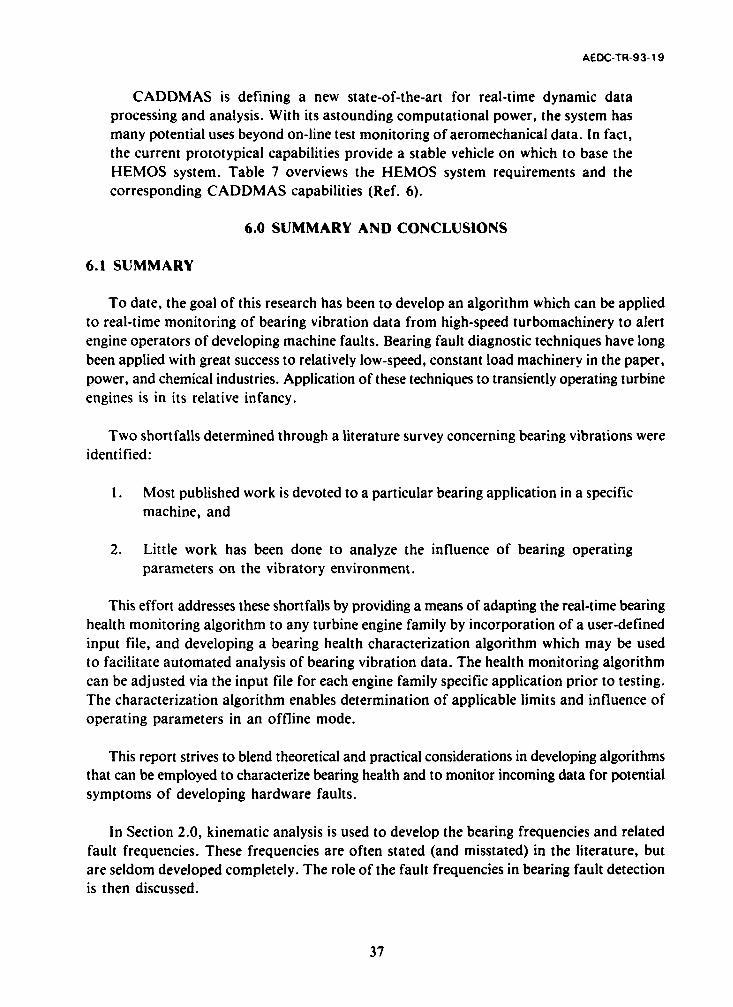
AEDC-TR-93-19

CADDMAS is defining a new state-of-the-art for real-time dynamic dataprocessing and analysis. With its astounding computational power, the system hasmany potential uses beyond on-line test monitoring of aeromechanical data. In fact,the current prototypical capabilities provide a stable vehicle on which to base theHEMOS system. Table 7 overviews the HEMOS system requirements and thecorresponding CADDMAS capabilities (Ref. 6).

6.0 SUMMARY AND CONCLUSIONS

6.1 SUMMARY

To date, the goal of this research has been to develop an algorithm which can be appliedto real-time monitoring of bearing vibration data from high-speed turbomachinery to alertengine operators of developing machine faults. Bearing fault diagnostic techniques have longbeen applied with great success to relatively low-speed, constant load machinery in the paper,power, and chemical industries. Application of these techniques to transiently operating turbineengines is in its relative infancy.

Two shortfalls determined through a literature survey concerning bearing vibrations wereidentified:

1. Most published work is devoted to a particular bearing application in a specificmachine, and

2. Little work has been done to analyze the influence of bearing operatingparameters on the vibratory environment.

This effort addresses these shortfalls by providing a means of adapting the real-time bearinghealth monitoring algorithm to any turbine engine family by incorporation of a user-definedinput file, and developing a bearing health characterization algorithm which may be usedto facilitate automated analysis of bearing vibration data. The health monitoring algorithmcan be adjusted via the input file for each engine family specific application prior to testing.The characterization algorithm enables determination of applicable limits and influence ofoperating parameters in an offline mode.

This report strives to blend theoretical and practical considerations in developing algorithmsthat can be employed to characterize bearing health and to monitor incoming data for potentialsymptoms of developing hardware faults.

In Section 2.0, kinematic analysis is used to develop the bearing frequencies and relatedfault frequencies. These frequencies are often stated (and misstated) in the literature, butare seldom developed completely. The role of the fault frequencies in bearing fault detectionis then discussed.

37

AEDC-TR-93-19

The physical quantities of vibration and the investigation of the interrelationships ofdisplacement, velocity, and acceleration are defined and examined in Section 3.0. Examinationof these mathematical relationships revealed the need for the health monitoring algorithmto be capable of incorporation of all three quantities into the logic. Frequency dependencyand availability of proximity probes, velocity pick-ups, and accelerometers for turbine engineapplication necessitate this algorithm capability.

Additionally, Section 3.0 reviewed data presentation alternatives, primary bearing responsesand the associated excitation sources, potential "health hazard" frequency responses, andlimit application methodologies. The inherent advantages of using the amplitude versus K-Factor approach to limit application over the sliding mask approach were developed anddiscussed. Further, an overview of the bearing health monitoring algorithm and its inclusivecontinuous and trend modes of operation was introduced.

Analytical results from a single bearing housing mounted accelerometer were providedin Section 4.0. Data from accelerations and decelerations at 21 flight conditions were manually

analyzed to develop trends of vibration amplitude with respect to various engine operatingparameters. The enormity of this effort along with the realization that most turbine enginetest articles are equipped with up to 12 vibration sensors and encompass 50 to 60 flightconditions illustrate the need for automating this analysis process. Preliminary programmingof the characterization algorithm has been accomplished in FY93, and adaptation to theCADDMAS software will begin in FY94.

A culmination of research and analysis efforts was reached in Section 5.0 for development

of bearing health criteria. The need for statistically categorizing engine family vibrationcharacteristics was addressed, and a means of developing this statistical analysis was includedas the bearing health characterization algorithm. Brief discussions of the role of operatingenvironment on vibration characteristics and the significance of fault frequency combinationswere then incorporated. A logic flow diagram for the actual real-time automated bearinghealth monitoring algorithm was presented and discussed. Finally, the role of CADDMAScapabilities versus HEMOS system requirements was introduced.

6.2 CONCLUSIONS

First, feasibility of developing an automated bearing health monitoring system throughvibration analysis has been established. A literature survey revealed successes in the realmof monitoring for turbine engine faults through vibration investigation in both online andoffline modes. Significant obstacles and lessons learned were also gleaned from the survey.Correct pre-teardown and post-mortem fault diagnoses, in which conditions leading to

38

AEOC-TR-93- 19

catastrophic failure were identified minutes and even hours prior to the failure event, lentparticular credence to system feasibility.

Second, the relationships of peak-to-peak displacement, peak velocity, and peakacceleration indicate a significant influence of frequency of vibration on the measuredamplitudes. Displacement, for example, is an excellent measure (f vibration at lowerfrequencies, but becomes practically useless at frequencies above 1000 Hz. Hence, eachmeasurement quantity of vibration has a range of frequencies over which satisfactory amplituderesolution is maintained. Experience in turbine engine bearing vibration data analysis suggests

the following frequency ranges:

displacement - 0 to 500 Hz,

velocity - 200 to 1200 Hz, and

acceleration - 800 to 10,000 Hz.

Importantly, most engine-mounted accelerometers provide a flat frequency response from0 to 10,000 Hz. This means that amplitude outputs are reliable over this range. At lowerfrequencies, however, note that units of displacement or velocity give a more intuitive feelfor the vibration amplitude. The algorithms require special attention to the vibration sensorsinstalled and the inherent advantages and disadvantages when specifying applicable alert andalarm limits.

Third, the K-Factor approach to limit application is a key development. Using thismethodology, statistical analyses can be conducted which will provide meaningful amplitudealert and alarm limits as a function of constant K-Factori. This eliminates the hugedevelopment task associated with programming alert and alarm limits, which are functionsof the frequencies of vibration (i.e., the sliding mask).

Fourth, analysis of a single bearing-mounted accelerometer responses to accelerationsand decelerations at a variety of flight conditions yielded significant results. Though trendingstudies of the influence of several operating parameters were accomplished, the primary"excitation source was always rotor unbalance (i.e., the highest amplitudes of vibration werealways measured at the highest rotor speeds, regardless of operating environment). If provenusing the bearing health characterization algorithm, this postulation may greatly simplifythe real-time health monitoring methodology.

Fifth, two algorithms were developed. The first, bearing health characterization algorithm,should allow automated analysis to statistically band common responses for a given engine

39

AEDC-TR-93-19

component (e.g., bearing) across a wide array of operating conditions and speeds. From thisanalysis, it is judged that meaningful alert and alarm limits can be specified for individual

engine families and sensor placement locations. The second algorithm, real-time bearing health

monitoring algorithm, can be further developed to provide a means of real-time avoidanceof catastrophic failures by alerting engine operators to potential developing hardware faults.

Future HEMOS plans include algorithm expansion to encompass all engine-mounted vibration

sensors (i.e., case, gear box, etc.) and incorporate transient digital signals to enhance overall

engine health determination.

Finally, the efforts presented in this report establish the methodologies by which meaningful

characterization of relative bearing health may be achieved. The algorithms must next be

automated and refined, and in-depth analyses must be conducted for a variety of engine

families. The ultimate goal of saving turbine engines from total self destruction appears tobe within reach. The algorithms developed in this report should provide a means of reach-

ing that goal.

REFERENCES

1. Braun, S. Mechanical Signature Analysis: Theory aaa Applications. London: AcademicPress, 1986.

2. Blake, Michael P. and William S. Mitchell. Vibration and Acoustic MeasurementHandbook. New York-Washington: Spartan Books, 1972.

3. Smith, Richard L. "Rolling Element Bearing Diagnostics with Lasers, Microphones,

and Accelerometers." 46th Meeting of the Mechanical Failures Prevention Group, Va.

Beach, VA, April 7-9, 1992.

4. Pettigrew, James L. "Diagnostics Look at Engine Condition." 44th Meeting of the

Mechanical Failures Prevention Group, Virginia Beach, VA, April 3-5, 1990.

5. Carr, H. R. "UK Military Engine Vibration Monitoring Experience." SAE E-32 Engine

Health Monitoring Committee Symposium-Vibration Monitoring and Analysis, Zurich,Switzerland, October 23-24, 1990.

6. Hite, S. W. "Real Time Vibration Health Monitoring For Transiently Operating High-Speed Turbomachinery." 47th Meeting of the Mechanical Failures Prevention Group,

Virginia Beach, VA, April 13-16, 1993.

40

AEDC-TR-93-19

7. Li, C. J. and J. Ma. "Bearing Localized Defect Detection Through WaveletDecomposition of Vibrations." 46th Meeting of the Mechanical Failures PreventionGroup, Virginia Beach, VA, April 7-9, 1992.

8. Harris, T. A. Rolling Bearing Analysis. Second Edition. New York: John Wiley andSons, 1984.

9. White, R. F. "Vibratory Velocity; A Measure of the Destructive Potential of Vibration."Allison Laboratory Report, A-9628, August 1970.

10. Collatz, Lothar. Functional Analysis and Numerical Mathematics. New York-London:Academic Press, 1966.

11. Jackson, C. J. The Practical Vibration Primer. Second Printing. Houston: GulfPublishing Company, 1981.

41

AEDC-TR-93-19

I IIIII

0

I..

0

State "A"

Time --

Figure 1. Phases of machine deterioration.

43

AEDC-TR-93-19

:I!·

Figure 2. Failed ball elem~jnt thrust bearing.

44

Ii ~

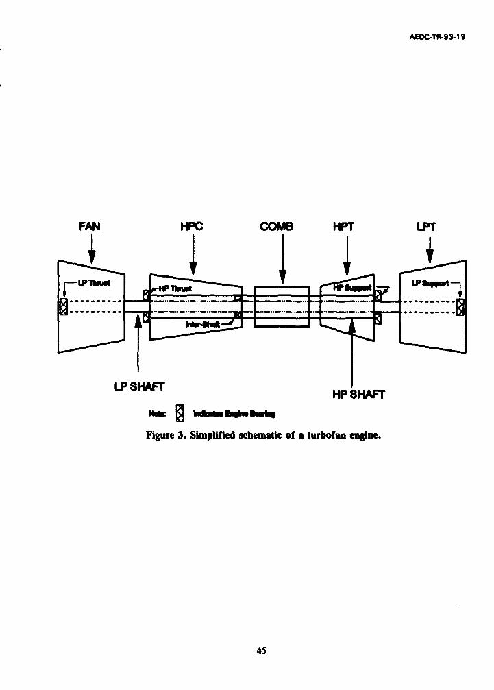
AEDC-TR-93-19

FAN HPC COMB HPT LPT

V LPThrnihn L MP-- ----'• ---------------: .. ....... _. _ " ....... -- -----

LP SHAFT

Figure 3. Simplified schematic of a turbofan engine.

45

~ 0'\

Rolling

Outer

Race

Figure 4. Rolling element bearing geometry and motion.

» m o ()

~ ::0 cD 'f ~

c.o

AEOC-TRS3- 19

3ix

Due to ResidualCL VMass Unbalance

CL 2- • Harmonics MayE be Present

S~2X

3XE

100 200 300

Frequency, Hz

Figure 5. Typical "healthy" bearing spectrum.

1X FTF and Sidebands

Indicative of Cracked CageC.

S1X - lX + S2X

FTF FTF

-1 FTF / 3XE

"Freuenc, HzFigure 6. Deteriorated bearing spectrum.

47

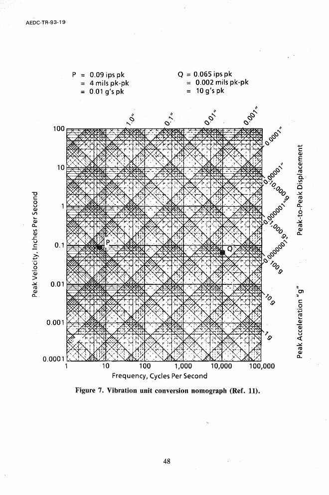
AEDC-TR-93-19

-u c o u ClJ

1.1\ L.

ClJ a.. V\ ClJ -c u c

>. +oJ 'u o ClJ > .:x co ClJ a..

P = 0.09 ips pk = 4 mils pk-pk = 0.01 9'S pk

Q = 0.065 ips pk = 0.002 mils pk-pk = 10 9'S pk

0.0001~~~~~~~~~~~~~~~~~~~~ 1 10 100 1,000 10,000 100,000

Frequency, Cycles Per Second

Figure 7. Vibration unit conversion nomograph (Ref. 11).

48

+oJ C QI

E QI u co a. . V\

6 .:x co QI a..

I

o ~ ~ co QI a..

::: Ol

::: c o

'';; co L.

QI

QI u u <{ .:x co QI a..

AE

DC

-TR

-93-19S

IJ 0

Leii

CL A

.... .....

s_________________________

00 C

dw

-N

qw

Nd-d U

lWepnu~

y N-N

qw'eq~

49I

AED

C-TR

-93- 19

4.0~

9L

=I -I

LU

bigi

50

AEDC-TR-93-19

4. Shift in Critical Speedand Amplitude

C.4

Es

C#

-- 4

44•

Sa N

* 4

0 6

* 4

4 -

4 S

-oo

4 - -#

0.6.

55

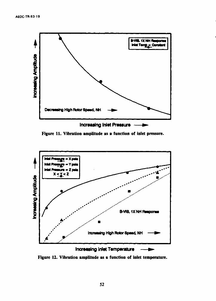
AEDC-TR-93-1 9

ISVNISXNHRb poi

DueCMing High RoWo Speed, NH w~

Incrasing Inlet Pressure --- w

Figure 11. Vibration amplitude as a function of inlet pressure.

w net Prewui - z Pesi

I~ ~ 1Cncras High RotorBSplXNHR.-Do-u~

IncreasIng Inlet Temperature '

Figure 12. Vibration amplitude as a function of inlet temperature.

52

AEDC-TR-93-19

Wbi Teonj. bwftIII

Increasng Lube Tank Pressre - No

Figure 13. Vibration amplitude as a function of lube tank pressure.

I,~r Irx.t_ Twpw.nT

Increasing Lube Tank Temperature -*

Figure 14. Vibration amplitude as a function of lube tank temperature.

53

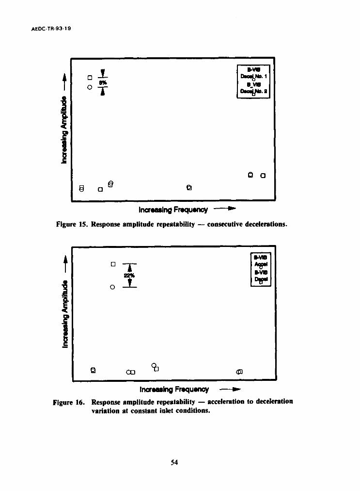
AEDC-TR-93-19

&II0 "No I• ,

0ILV

Oo@ a a

Incremsing Frequency -00,

Figure 15. Response amplitude repeatability - consecutive decelerations.

riii

0-

*11Increasing Frequency

Figure 16. Response amplitude repeatability - acceleration to decelerationvariation at constant inlet conditions.

54

AEDC-TR-93-1 9

JFOR K -ITO JJ I 4J - NO. OF PARAMWTE111 TO PROCESS

I READ DATA IN I U - NO. OP DATA ENSEMLES IN_ _ _NO ACUSTO VN

OWT fAA [T VALID? STEP IYESn J - NO. OF SPECTRAL RESPO)NSES11

0VE1tFIEHOLDPROESSSTEP 2 K - NO0. OP UNMATCHED SPECTRAL

FINT REPONSES AFTER NOISE A 1STENIN ORDER INTERROGATION

READ INPUT FILE STEPS3v L - NO. OP UNMATCHE SPECTRAL

ORN I1 TO ZZ REPNSES AFTER IIN u.o. INEROGe~IATOt

NEXT POR - I OJU. - NO. OP UNMATCHED SPECTRAL. RESPONSES

O4TDATA fi - I rAbo? STEP 4 NN - NO. OP UNMATCHED SPECTRAL RESPONSES

COMPTE 1 FOREACH STEP AFTER SEAT FRED INTERROG10ATION

SCOMPRE f 10 W W-N NOR N? CTOMPREAIIKNIN STEPS

X STOR N. ... (L. IX , NW l V N..

10ftMTCBEAT 1 STE -SATHSTORE~~~~~STR Al. fl I0, IC. NU, STRNUfl 0 K U SE

IN ~ ~ ~~~~O ARRA TOR MACNNARA O ACi( STE 7ADM TP

MULTIPLES OF NL STORE Al. fl.10. NHI. NUMUTPEOFN

STORE ~ ~ ~ CMPT AND STORENI USTR l.f.1, HN

FOR ALL MATCLL1111 -IIBEAT i STEP 10

COMPUTE ANM STORERUNNING AVG. MAXC MODCH BASED ON ALL MATCHED 1t

PAN AND STD 0EVFOR ALL MODCH

FPRODUCE TABLE OP STATISTICAL PARAMETERS,) SEmP1HSORMAND CHRATERIZATION PLMl

Figure 17. Bearing health characterization algorithm flow chart.

55

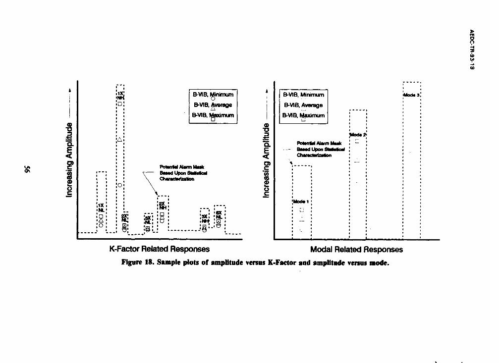
AED

C-TR

-93-19

JLl

ii

-- -

--

' V

.................................... 0

epni~ldwU

V B

useeJOul

1 0

.0 .l

-55

0U

: ~

o_.op

0,1

------------------------

I

epnIuidwv B

uiseajoul

56

AEDC-TR-93-19

READ DATA IN

NEXT DATA[-" I DATA VALID? STEP 1

IFFT PROCESSING STEP 2

READ DATA BASE STEP 3AND INPUT FILE

lXNL.1X N STEP 4

YES RED STORAG

STEP5 READ TREND DATA I - TREND REQUESTED?BASE AND INPUT FILEI YE OR NO

STeeP LO OSI N,1 NH COMPUTE KFACTOR FORVERSUS SPEED OR TIME EACH SPECTRAL RESPONISE] STEP 8

STEP 7 CMUEDVAININTERROGATE K-FACTOR VS STEP B* BASELINE FROM DATA BASE

PRINT HARD COPY ON DEMAND L YE

NOSOME K-FACTORS NOT RECOGNIZED? CIRCULAR FILE

LOGIC FOR BEARING SUBROUTINE YES

GO TO SUBROUTINE 'MODE' STEP 10COMPUTE THEORETICAL]

FAULT FREQUENCIES/ IEGO TO SUBROUTINE "BEATr STEP,11

COMPUTED THEORETICAL K-FACTORS G

t E FG-OTO SUBROUTINE 'RIDM STEP 13

STORGI ERMTNENTJ

Figure 19. Real-time bearing health monitoring algorithm flow chart.

57

AEDC-TR-93-19

Table 1. Rolling Element Bearing Defect Frequencies

Component Frequency Significance

Rolling element Vzfi(l -I,) Caused by an irreg-train defect (FTF) ularity of a rolling

element on the cage

Rolling element '/2m(dm/db)fi(V - 9t2) Irregularities alter-defect (BSF) nately strike inner

and outer races

Outer race (n/2)fi(l - ') Irregularity on racedefect (BPFO) generates impacting

with each rollingelement pass

Inner race (n/2)fi(l + it) Irregularity on racedefect (BPFI) generates impacting

with each rollingelement pass

Where fi = inner race frequency, N/60, in HzN = rotational speed in rpmm = number of rolling element irregularities

dm = mean bearing diameter (cf. Fig. 3)db = rolling element diameter (cf. Fig. 3)n = number of rolling elements

= (db/dm) cos 0= bearing contact angle (cf. Fig. 3)

58

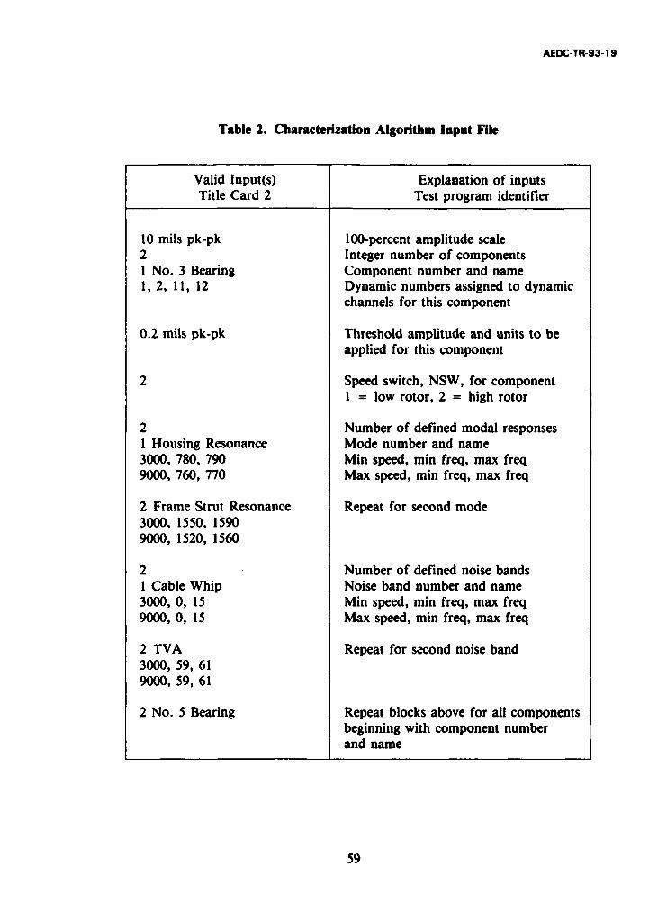
AEDC-TR-93-19

Table 2. Characterization Algorithm Input File

Valid Input(s) Explanation of inputsTitle Card 2 Test program identifier

10 mils pk-pk 100-percent amplitude scale2 Integer number of componentsI No. 3 Bearing Component number and name1, 2, 11, 12 Dynamic numbers assigned to dynamic

channels for this component

0.2 mils pk-pk Threshold amplitude and units to beapplied for this component

2 Speed switch, NSW, for componentI = low rotor, 2 = high rotor

2 Number of defined modal responses1 Housing Resonance Mode number and name3000, 780, 790 Min speed, min freq, max freq9000, 760, 770 Max speed, min freq, max freq

2 Frame Strut Resonance Repeat for second mode3000, 1550, 15909000, 1520, 1560

2 Number of defined noise bands1 Cable Whip Noise band number and name3000, 0, 15 Min speed, min freq, max freq9000, 0, 15 Max speed, min freq, max freq

2 TVA Repeat for second noise band3000, 59, 619000, 59, 61

2 No. 5 Bearing Repeat blocks above for all componentsbeginning with component numberand name

59

AEDC-TR-93,19

Table 3. Sample Statistical Output File

Output Data Significance

1 B-VIB Parameter number and name0.2 Threshold applied to dataIX NH Component of vibration389, 0.3, 2.8, 1.4, 0.67 No. of matched responses, min,

max, avg, and deviation2X NH Repeat for all engine order121, 0.4, 1.1, 0.8, 0.32 related responses

IX NL212, 0.6, 1.4, 0.8, 0.41

2X NL34, 0.3, 0.4, 0.4, 0.05

1 Housing Resonance Mode number and name166, 0.3, 0.5, 0.4, 0.10 No. of matched responses, min,

max, avg, and deviation

I Beat: (NH -NL)/60 Beat freq number and name59, 0.3, 0.7, 0.5, 0.20 No. of matched responses, min,

max, avg, and deviation

Random Random response indicator11, 0.3, 0.4, 0.4, 0.05 No. of random responses, min,

max, avg, and deviation

2 C-VIB Next parameter number and nameRepeat above beginning withthreshold

60

AEDC-TR-93-19

Table 4. Sample Histogram

Amplitude Range, No. of Matchespercent

0 - 20 118521 - 40 77041 - 60 21261 - 80 1181 - 100 2

Table S. Fault Frequency Combinations and Diagnoses

Defect or Condition Frequency Spectrum Shape Diagnosis

Inner race defect BPFI and mult Decreasing amplitude harmonics Shallow flaking

Inner race defects BPFI and mult Decreasing amplitude harmonics Failure imminent;and modulation at running speed shutdown required

Outer race defects BPFO and mult Decreasing amplitude harmonics Shallow flaking

Cage and outer BPFO and mult FTF modulation at higher Failure imminent;race defects and FTF frequencies shutdown required

Cage, balls, and BPFO and mult BPFO modulated by FTF Cage or rollerouter race defects and FTF defects

Outer race defects BPFO and mult Increasing amplitude harmonics Deep fatigue spall

Defects on inner BPFO and BPFI Bearing frequencies and sum Worsening defectsand outer races and difference frequencies

Inner race and BPFI and BSF Decreasing amplitude harmonics Worsening defectsball defect and BPFI modulated by BSF

Cage defect FTF and mult Steady amplitude harmonics of Badly worn orFTF cracked cage

Note: Adapted from: Eshleman, R. L. "Rolling Element Bearing Analysis." Vibration Institute:Machinery Vibration Analysis I, Course Notes, Nashville, Tn. November 17-20, 1987.

61

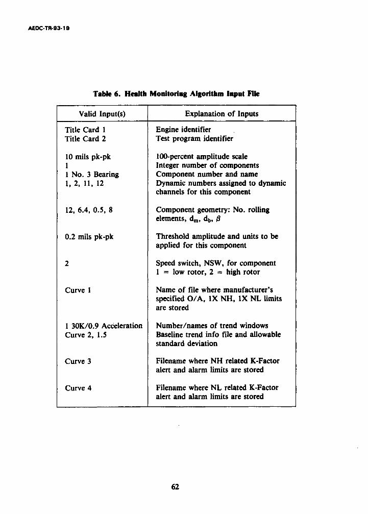
AEDC-TR-93-19

Table 6. Health Monitoring Algorithm Input File

Valid Input(s) Explanation of Inputs

Title Card 1 Engine identifierTitle Card 2 Test program identifier

10 mils pk-pk 100-percent amplitude scale1 Integer number of components1 No. 3 Bearing Component number and name1, 2, 11, 12 Dynamic numbers assigned to dynamic

channels for this component

12, 6.4, 0.5, 8 Component geometry: No. rollingelements, di, db, 0

0.2 mils pk-pk Threshold amplitude and units to beapplied for this component

2 Speed switch, NSW, for component1 = low rotor, 2 = high rotor

Curve I Name of file where manufacturer'sspecified O/A, IX NH, IX NL limitsare stored

1 30K/0.9 Acceleration Number/names of trend windowsCurve 2, 1.5 Baseline trend info file and allowable

standard deviation

Curve 3 Filename where NH related K-Factoralert and alarm limits are stored

Curve 4 Filename where NL related K-Factoralert and alarm limits are stored

62

AEDC-TR-93-19

Table 6. Concluded

Valid Input(s) Explanation of Inputs

1 Number of defined modal responses1 Housing Resonance Mode number and name

3000, 780, 790 Min speed, min freq, max freq

9000, 760, 770 Max speed, min freq, max freq

1.0, 1.5 mils pk-pk Specified alert and alarm limits

1 Beat: (NH - NL)/60 Numbers and names of defined beatfrequencies

0.6, 0.8 mils pk-pk Specified alert and alarm limits

FTF, 0.4, 0.8 Bearing fault frequency specifiedBSF, 0.4, 0.8 alert and alarm limitsBPFO, 0.4, 0.8BPFI, 0.4, 0.8

0.6, 1.2 mils pk-pk Specified alert and alarm limitsfor random vibration

1 Number of defined noise bands1 Cable Whip Noise band number and name3000, 0, 15 Min speed, min freq, max freq

9000, 0, 15 Max speed, min freq, max freq

63

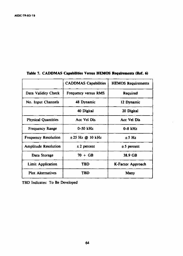
AEDC-TR-93-19

Table 7. CADDMAS Capabilities Versus HEMOS Requirements (Ref. 6)

CADDMAS Capabilities HEMOS Requirements

Data Validity Check Frequency versus RMS Required

No. Input Channels 48 Dynamic 12 Dynamic

40 Digital 20 Digital

Physical Quantities Acc Vel Dis Acc Vel Dis

Frequency Range 0-50 kHz 0-8 kHz

Frequency Resolution ±25 Hz @ 10 kHz ±5 Hz

Amplitude Resolution ± 2 percent ±5 percent

Data Storage 70 + GB 38.9 GB

Limit Application TBD K-Factor Approach

Plot Alternatives TBD Many

TBD Indicates: To Be Developed

64

AEDC-TR-93-19

NOMENCLATURE

Symbol Description

A Amplitude of vibration

a AccelerationAcc Acceleration

AEDC Arnold Engineering Development Center

B Peak displacement

BEATf Beat frequency

B-VIB Bearing housing mounted accelerometer

BPFI Ball passing frequency-inner race

BPFO Ball passing frequency-outer race

BSF Ball spin frequency (also fb)

03 Bearing contact angle

CADDMAS Computer Assisted Dynamic Data Monitoring and Analysis System

COMB Combustion chamber

cps Cycles per second (also Hz)

CRT Cathode ray tube

D Time-dependent displacement of a body

d Peak-to-peak displacement

db Rolling element diameterdi Inner race diameter

Disp Displacement

dm Bearing mean (or pitch) diameter

DN Bearing diameter times running speed

do Outer race diameter

DOTP Directorate of Technology-Propulsion Division

ETF Engine Test Facility

FFT Fast Fourier Transform

FTF Fundamental train frequency (also fio)

freq Frequency (also f)f Frequency (also freq)

65

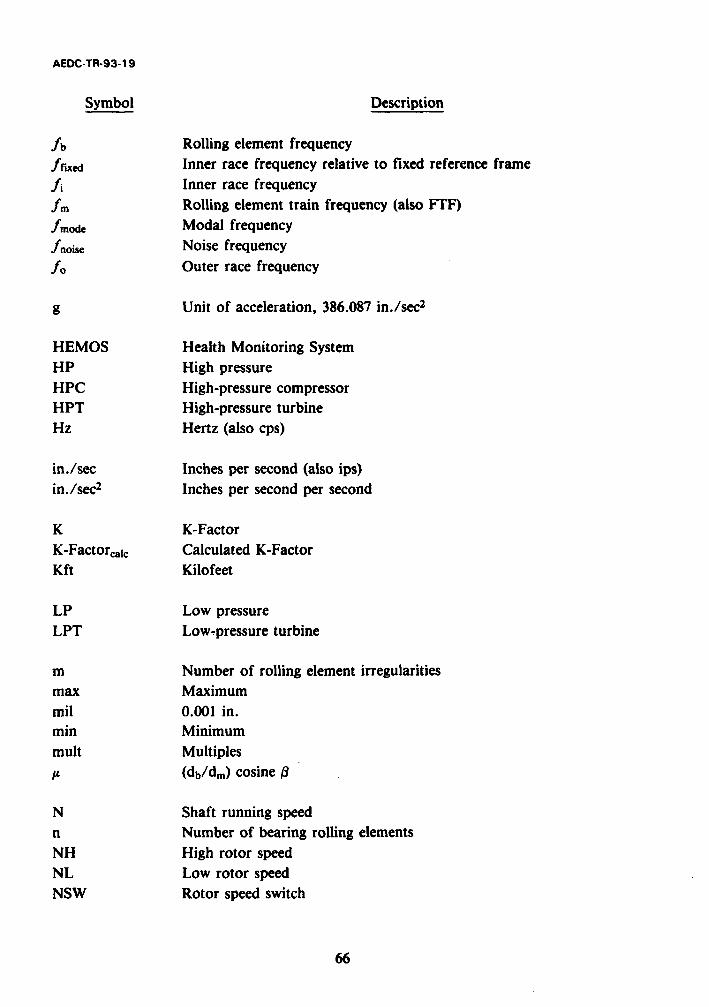
AEDC-TR-93-19

Symbol Description

Ab Rolling element frequency

fAxed Inner race frequency relative to fixed reference framefi Inner race frequency

fm Rolling element train frequency (also FTF)

fmode Modal frequency'noise Noise frequency

Ao Outer race frequency

g Unit of acceleration, 386.087 in./sec2

HEMOS Health Monitoring SystemHP High pressureHPC High-pressure compressorHPT High-pressure turbineHz Hertz (also cps)

in./sec Inches per second (also ips)in./sec2 Inches per second per second

K K-FactorK-Factorcac Calculated K-FactorKft Kilofeet

LP Low pressureLPT Low~pressure turbine

m Number of rolling element irregularitiesmax Maximummil 0.001 in.min Minimummult Multiples1A (db/dm) cosine •

N Shaft running speedn Number of bearing rolling elementsNH High rotor speedNL Low rotor speedNSW Rotor speed switch

66

AEDC-TR-93-19

Symbol Description

O/A Overall vibration

pk Peakpk-pk Peak to peakPTO Power take-off

r Distance from axis of rotationri Distance from shaft center to point on surface of inner racermi Distanqe from rolling element center to point of contact with inner

racerms Root-mean-squarero Distance from shaft center to point on surface of outer race

sps Samples per secondSTD DEV Standard deviation

TVA Tennessee Valley Authority

v VelocityVb Rolling element velocityVel Velocityvi Inner race velocityVm Rolling element train velocityVo Outer race velocityVpk-pk Peak-to-peak voltage

w Angular velocityWb Rolling element angular velocityWrixed Inner race angular velocity relative to fixed reference framewi Inner race angular velocitywm Rolling element train angular velocityWmi Rolling element train angular velocity relative to the inner raceWo Outer race angular velocity

1/rev Once per revolution

IX, 2X, 3X, Multiples of running speed

67