an algorithm for denoising and compression in wireless
TRANSCRIPT

Chapter 9
© 2012 Sheybani, licensee InTech. This is an open access chapter distributed under the terms of the Creative Commons Attribution License (http://creativecommons.org/licenses/by/3.0), which permits unrestricted use, distribution, and reproduction in any medium, provided the original work is properly cited.
An Algorithm for Denoising and Compression in Wireless Sensor Networks
Ehsan Sheybani
Additional information is available at the end of the chapter
http://dx.doi.org/10.5772/48518
1. Introduction
Many wireless sensor network datasets suffer from the effects of acquisition noise, channel
noise, fading, and fusion of different nodes with huge amounts of data. At the fusion center,
where decisions relevant to these data are taken, any deviation from real values could affect
the decisions made. We have developed computationally low power, low bandwidth, and
low cost filters that will remove the noise and compress the data so that a decision can be
made at the node level. This wavelet‐based method is guaranteed to converge to a
stationary point for both uncorrelated and correlated sensor data. Presented here is the
theoretical background with examples showing the performance and merits of this novel
approach compared to other alternatives.
Noise (from different sources), data dimension, and fading can have dramatic effects on the
performance of wireless sensor networks and the decisions made at the fusion center. Any
of these parameters alone or their combined result can affect the final outcome of a wireless
sensor network. As such, total elimination of these parameters could also be damaging to
the final outcome, as it may result in removing useful information that can benefit the
decision making process. Several efforts have been made to find the optimal balance
between which parameters, where, and how to remove them. For the most part, experts in
the field agree that it is more beneficial to remove noise and/or compress data at the node
level [Closas, P., 2007], [Yamamoto, H., 2005], [Son, S.‐H., 2005]. This is mainly stressed so
that the low power, low bandwidth, and low computational overhead of the wireless sensor
network node constraints are met while fused datasets can still be used to make reliable
decisions [Abdallah, A., 2006], [Schizas, I.D., 2006], [Pescosolido, L., 2008].
Digital signal processing algorithms, on the other hand, have long served to manipulate
data to be a good fit for analysis and synthesis of any kind. For the wireless sensor networks

Wireless Sensor Networks – Technology and Applications 188
a special wavelet‐based approach has been considered to suppress the effect of noise and
data order. One of the advantages of this approach is in that one algorithm serves to both
reduce the data order and remove noise. The proposed technique uses the orthogonality
properties of wavelets to decompose the dataset into spaces of coarse and detailed signals.
With the filter banks being designed from special bases for this specific application, the
output signal in this case would be components of the original signal represented at
different time and frequency scales and translations. A detailed description of the
techniques follows in the next section.
2. Wavelet‐based transforms
Traditionally, Fourier transform (FT) has been applied to time‐domain signals for signal
processing tasks such as noise removal and order reduction. The shortcoming of the FT is in
its dependence on time averaging over entire duration of the signal. Due to its short time
span, analysis of wireless sensor network nodes requires resolution in particular time and
frequency rather than frequency alone. Wavelets are the result of translation and scaling of a
finite‐length waveform known as mother wavelet. A wavelet divides a function into its
frequency components such that its resolution matches the frequency scale and translation. To
represent a signal in this fashion it would have to go through a wavelet transform. Application
of the wavelet transform to a function results in a set of orthogonal basis functions which are
the time‐frequency components of the signal. Due to its resolution in both time and frequency
wavelet transform is the best tool for detection and classification of signals that are non‐
stationary or have discontinuities and sharp peaks. Depending on whether a given function is
analyzed in all scales and translations or a subset of them the continuous (CWT), discrete
(DWT), or multi‐resolution wavelet transform (MWT) can be applied.
An example of the generating function (mother wavelet) based on the Sinc function for the
CWT is:
2 2 – t Sinc t Sinc t (2 ) ( )Sin t Sin t
t
(1)
The subspaces of this function are generated by translation and scaling. For instance, the
subspace of scale (dilation) a and translation (shift) b of the above function is:
,
1( ) ( )a b
t bt
aa
(2)
When a function x is projected into this subspace, an integral would have to be evaluated to
calculate the wavelet coefficients in that scale:
, ,{ }( , ) , ( ) ( )a b a bR
WT x a b x x t t dt (3)
And therefore, the function x can be shown in term of its components:

An Algorithm for Denoising and Compression in Wireless Sensor Networks 189
,( ) { }( , ). ( ) .a a bR
x t WT x a b t db (4)
Due to computational and time constraints it is impossible to analyze a function using all of
its components. Therefore, usually a subset of the discrete coefficients is used to reconstruct
the best approximation of the signal. This subset is generated from the discrete version of
the generating function:
/ 2, .m m
m n t a a t nb (5)
Applying this subset to a function x with finite energy will result in DWT coefficients from
which one can closely approximate (reconstruct) x using the coarse coefficients of this
sequence:
, ,( ) , . ( ).m n m nm Zn Z
x t x t
(6)
The MWT is obtained by picking a finite number of wavelet coefficients from a set of DWT
coefficients. However, to avoid computational complexity, two generating functions are
used to create the subspaces:
Vm Subspace:
/ 2, 2 2m m
m n t t n (7)
And Wm Subspace:
/ 2, 2 2 .m m
m n t t n (8)
From which the two (fast) wavelet transform pairs (MWT) can be generated:
( ) 2 (2 )nn Z
t h t n
(9)
and
( ) 2 (2 )nn Z
t g t n
(10)
In this paper the DWT has been used to suppress noise and reduce order of data in a
wireless sensor network. Due to its ability to extract information in both time and frequency
domain, DWT is considered a very powerful tool. The approach consists of decomposing the
signal of interest into its detailed and smoothed components (high‐and low‐frequency). The
detailed components of the signal at different levels of resolution localize the time and

Wireless Sensor Networks – Technology and Applications 190
frequency of the event. Therefore, the DWT can extract the coarse features of the signal
(compression) and filter out details at high frequency (noise). DWT has been successfully
applied to system analysis for removal of noise and compression [Cohen, I., 1995],
[Daubechies, I., 1992]. In this paper we present how DWT can be applied to detect and filter
out noise and compress signals. A detailed discussion of theory and design methodology for
the special‐purpose filters for this application follows.
3. Theory of DWT‐based filters for noise suppression and order
reduction
DWT‐based filters can be used to localize abrupt changes in signals in time and frequency.
The invariance to shift in time (or space) in these filters makes them unsuitable for
compression problems. Therefore, creative techniques have been implemented to cure this
problem [Liang, J., 1996], [Cohen, I., 1995], [Daubechies, I., 1992], [Coifman, R., 1992],
[Mallat, S., 1991], [Mallat, S., 1992]. These techniques range in their approach from
calculating the wavelet transforms for all circular shifts and selecting the “best” one that
minimizes a cost function [Liang, J., 1996], to using the entropy criterion [Coifman, R., 1992]
and adaptively decomposing a signal in a tree structure so as to minimize the entropy of the
representation. In this paper a new approach to cancellation of noise and compression of
data has been proposed. The discrete Meyer adaptive wavelet (DMAW) is both translation‐
and scale‐invariant and can represent a signal in a multi‐scale format. While DMAW is not
the best fit for entropy criterion, it is well suited for the proposed compression and
cancellation purposes [Mallat, S., 1992].
The process to implement DMAW filters starts with discritizing the Meyer wavelets defined
by wavelet and scaling functions as:
( ) 2 (2 )nn Z
t h t n
(11)
and
( ) 2 (2 )nn Z
t g t n
(12)
The masks for these functions are obtained as:
1 1
(0), ( ),....., ( )2 2m m
M
(13)
and
1
0,0,...,0, (0), ( ),....., ( ) .N
(14)

An Algorithm for Denoising and Compression in Wireless Sensor Networks 191
As these two masks are convolved, the generating function (mother wavelet) mask can be
obtained as:
( ) ( ).2mk
F M k N (15)
Where for every integer k, integers 1 2, ,.....,k k kqn n n can be found to satisfy the inequality:
3
3 (1 ).2 2
ki m m
kn i q
(16)
The corresponding values from mother wavelet mask can then be taken to calculate:
/22( )2
kmk ii m
F
,
where ( )2 (1 )k k mi in k i q
and
,
1
.q
m k kni i
i
cc
(17)
Decomposing the re‐normalized signal , ( )m kc
k Z
according to the conventional DWT,
will result in the entire DMAW filter basis for different scales:
1, 1, 2, 2, 0, 0,, , , ,...., ,m k m k m k m k k kc d c d c d
(18)
4. Experimental results
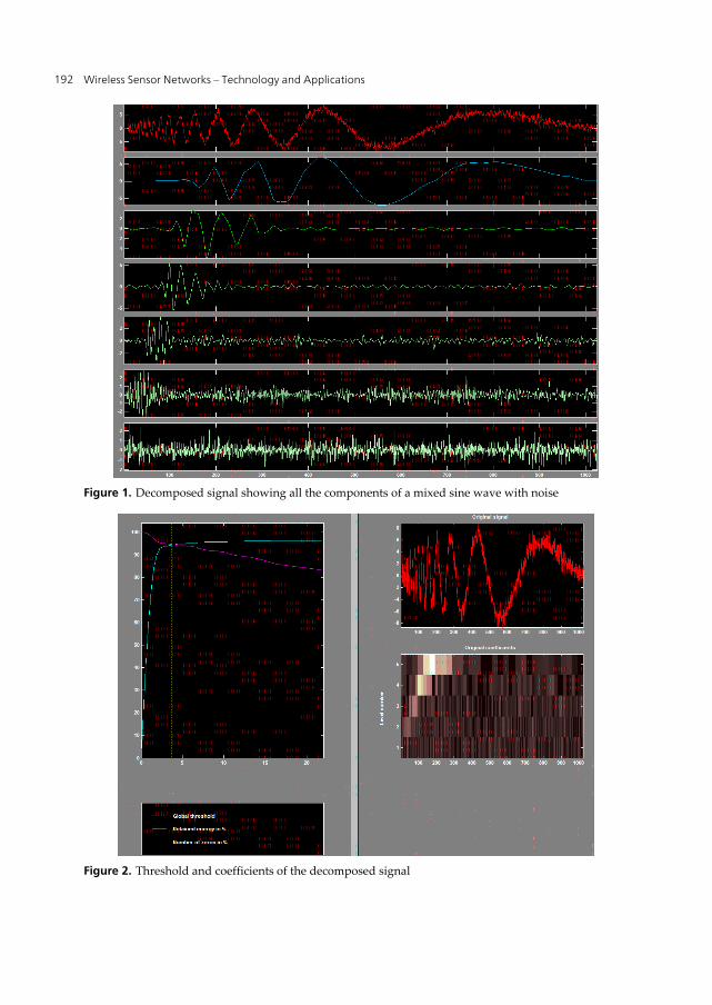
Figures 1, 2, and 3 show the experimental results for the application of the proposed filter
banks to a noisy sinusoidal signal. As is evident from these figures, a signal can be
decomposed in as many levels as desired by the application and allowed by the
computational constraints. Levels shown from top to bottom represent the coarse to detailed
components of the original signal.
Once the signal is decomposed to its components, it is easy to do away with pieces that are
not needed. For instance, noise, which is the lower most signal in Figure 1 can be totally
discarded. On the other hand, if compression is necessary, all but the coarse component
(upper most element, below the original signal) can be kept and the rest of the modules
discarded. This signal alone is a fairly good approximation of the original signal. Figure 2
shows the thresholds and coefficients of the signal being filtered.
Wireless Sensor Networks – Technology and Applications 192
Figure 1. Decomposed signal showing all the components of a mixed sine wave with noise
Figure 2. Threshold and coefficients of the decomposed signal

An Algorithm for Denoising and Compression in Wireless Sensor Networks 193
Figure 3. Histogram and cumulative histogram of the signal
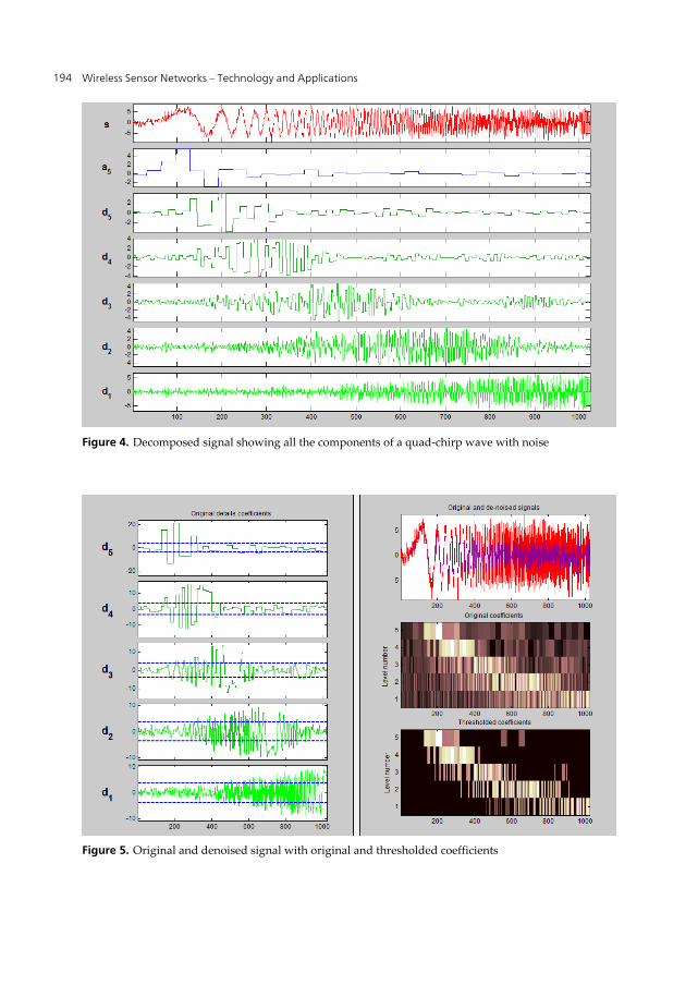
Figure 3 shows the histogram (frequency of components distribution) of the signal. For
comparison purposes the same filter banks have also been applied to a quad‐chirp signal
with noise and the results are shown in Figures 4‐9. The denoised and compressed versions
of the signal have been computed and plotted. In each case the coefficients that have
remained intact for denoising and compression have also been displayed. Finally, in Figures
7‐25 the histogram for the denoised and compressed quad‐chirp, auto‐regressive, white
noise, and step signals have been compared to the original signal. The effectiveness of the
proposed filter banks and their capability to maintain the important components of the
original signal is evident in these figures.
Wireless Sensor Networks – Technology and Applications 194
Figure 4. Decomposed signal showing all the components of a quad‐chirp wave with noise
Figure 5. Original and denoised signal with original and thresholded coefficients

An Algorithm for Denoising and Compression in Wireless Sensor Networks 195
Figure 6. Threshold and coefficients of the decomposed signal showing retained energy and number of
zeros
Figure 7. Histogram and cumulative histogram of the original quad‐chirp signal
Wireless Sensor Networks – Technology and Applications 196
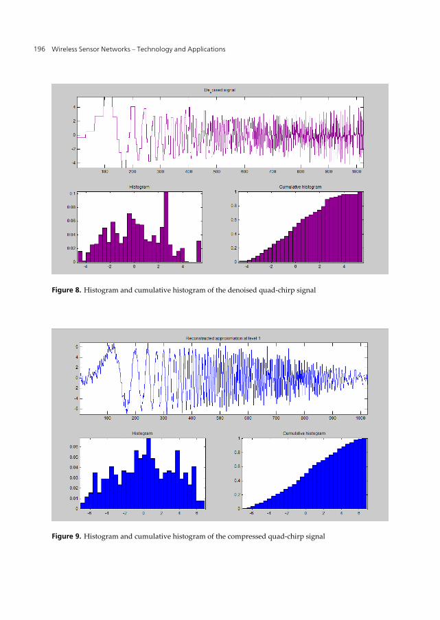
Figure 8. Histogram and cumulative histogram of the denoised quad‐chirp signal
Figure 9. Histogram and cumulative histogram of the compressed quad‐chirp signal
An Algorithm for Denoising and Compression in Wireless Sensor Networks 197
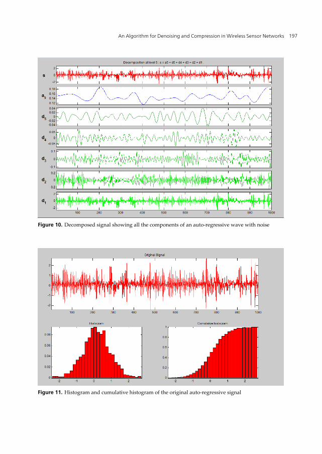
Figure 10. Decomposed signal showing all the components of an auto‐regressive wave with noise
Figure 11. Histogram and cumulative histogram of the original auto‐regressive signal

Wireless Sensor Networks – Technology and Applications 198
Figure 12. Threshold and coefficients of the decomposed signal showing retained energy and number
of zeros
Figure 13. Original and denoised signal with original and thresholded coefficients

An Algorithm for Denoising and Compression in Wireless Sensor Networks 199
Figure 14. Decomposed signal showing all the components of white noise
Figure 15. Histogram and cumulative histogram of the original white noise signal
Wireless Sensor Networks – Technology and Applications 200
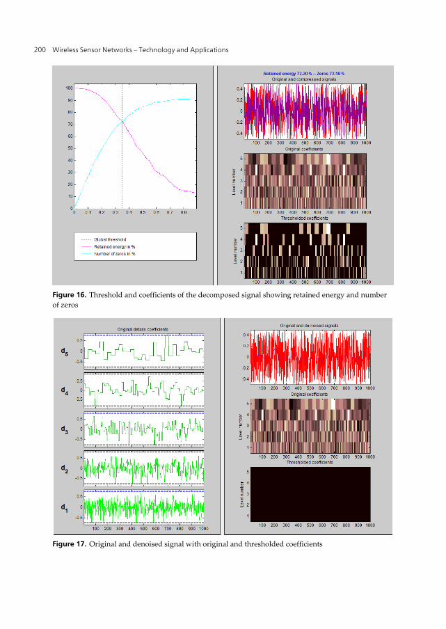
Figure 16. Threshold and coefficients of the decomposed signal showing retained energy and number
of zeros
Figure 17. Original and denoised signal with original and thresholded coefficients

An Algorithm for Denoising and Compression in Wireless Sensor Networks 201
Figure 18. Decomposed signal showing all the components of a doppler wave with noise
Figure 19. Histogram and cumulative histogram of the original doppler signal

Wireless Sensor Networks – Technology and Applications 202
Figure 20. Threshold and coefficients of the decomposed signal showing retained energy and number
of zeros
Figure 21. Original and denoised signal with original and thresholded coefficients

An Algorithm for Denoising and Compression in Wireless Sensor Networks 203
Figure 22. Decomposed signal showing all the components of a step signal
Figure 23. Histogram and cumulative histogram of the original step signal
Wireless Sensor Networks – Technology and Applications 204
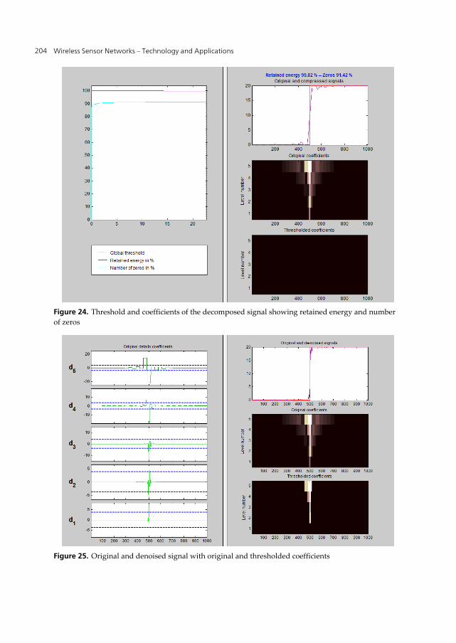
Figure 24. Threshold and coefficients of the decomposed signal showing retained energy and number
of zeros
Figure 25. Original and denoised signal with original and thresholded coefficients

An Algorithm for Denoising and Compression in Wireless Sensor Networks 205
5. Conclusions and future work
As expected from the theory, the DMAW filters performed well under noisy conditions in a
wireless sensor network. The decomposed signal could be easily freed up from noise and
reduced down to its coarse component only. This could be reduction by several orders of
magnitude in some cases. Future plans include the application of these filters to fused
datasets and comparison between the two approaches. Additionally, the results of these
study can be used in the decision making stage to realize the difference this approach can
make in speed and efficiency of this process.
Future work will address issues such as characterizing the parameters for simulation and
modeling of the proposed filter for WSN; showing how complex examples with correlated
sensor data will be filtered for redundancy; comparing the proposed approach with other
similar approaches and giving comparative results to support the claimed advantages, both
theoretically and experimentally.
Author details
Ehsan Sheybani
Virginia State University, Petersburg, VA, USA
6. References
Abdallah, A., Wolf, W., “Analysis of Distributed Noise Canceling”, Distributed Frameworks
for Multimedia Applications, 2006. The 2nd International Conference on, May 2006, pp. 1–7.
Closas, P., Calvo, E., Fernandez‐Rubio, J.A., Pages‐Zamora, A., “Coupling noise effect in
self‐synchronizing wireless sensor networks”, Signal Processing Advances in Wireless
Communications, 2007. SPAWC 2007. IEEE 8th Workshop on, 17‐20 June 2007, pp.1‐5.
Cohen, I., S. Raz, and D. Malah, “Shift invariant wavelet packet bases,” in Proc. 20th IEEE
Int. Conf. Acoustics, Speech, Signal Processing, Detroit, MI, May 8–12, 1995, pp. 1081–1084.
Coifman, R.R. and M. V. Wickhauser, “Entropy‐based algorithms for best basis selection,”
IEEE Trans. Inform. Theory, vol. 38, pp. 713–718, Mar. 1992.
Daubechies, I., “Ten lecture on wavelet,” in CBMS‐NSF Regional Conference Series in Applied
Mathematics. Philadelphia, PA: SIAM, 1992.
Liang, J. and T.W. Parks, “A translation invariant wavelet representation algorithm with
applications,” IEEE Trans. Signal Processing, vol. 44, pp. 225–232, Feb. 1996.
Mallat, S., “Zero‐crossings of a wavelet transform,” IEEE Trans. Inform. Theory, vol. 37, pp.
1019–1033, July 1991.
Mallat, S. and S. Zhang, “Characterization of signals from multiscale edges,” IEEE Trans.
Pattern Anal. Machine Intell., vol. 14, pp. 710–732, July 1992.
Pescosolido, L., Barbarossa, S., Scutari, G., “Average consensus algorithms robust against
channel noise”, Signal Processing Advances in Wireless Communications, 2008. SPAWC
2008. IEEE 9th Workshop on, 6‐9 July 2008, pp. 261–265.

Wireless Sensor Networks – Technology and Applications 206
Schizas, I.D., Giannakis, G.B., ”Zhi‐Quan Luo Optimal Dimensionality Reduction for Multi‐
Sensor Fusion in the Presence of Fading and Noise”, Acoustics, Speech and Signal
Processing, 2006. ICASSP 2006 Proceedings. 2006 IEEE International Conference on, 14‐19
May 2006, Vol. 4, pp. IV – IV.
Son, S.‐H., Kulkarni, S.R., Schwartz, S.C., Roan, M., “Communication‐estimation tradeoffs in
wireless sensor networks”, Acoustics, Speech, and Signal Processing, 2005. Proceedings.
(ICASSP apos;05). IEEE International Conference on, Volume 5, Issue , 18‐23 March 2005,
pp. 1065‐1068, Vol. 5.
Yamamoto, H., Ohtsuki, T., “Wireless sensor networks with local fusion:, Global
Telecommunications Conference, 2005. GLOBECOM ʹ05. IEEE, 28 Nov.‐2 Dec. 2005, Vol. 1,
pp 5.