an algebraic multigrid method for - arxiv · an algebraic multigrid method for quadratic finite...

AN ALGEBRAIC MULTIGRID METHOD FORQUADRATIC FINITE ELEMENT EQUATIONS OFELLIPTIC AND SADDLE POINT SYSTEMS IN 3D

HUIDONG YANG

Abstract. In this work, we propose a robust and easily imple-mented algebraic multigrid method as a stand-alone solver or a pre-conditioner in Krylov subspace methods for solving either symmet-ric and positive definite or saddle point linear systems of equationsarising from the finite element discretization of the vector Lapla-cian problem, linear elasticity problem in pure displacement andmixed displacement-pressure form, and Stokes problem in mixedvelocity-pressure form in 3D, respectively. We use hierarchical qua-dratic basis functions to construct the finite element spaces. Anew heuristic algebraic coarsening strategy is introduced for con-struction of the hierarchical coarse system matrices. We focus onnumerical study of the mesh-independence robustness of the alge-braic multigrid and the algebraic multigrid preconditioned Krylovsubspace methods.

1. Introduction

Compared to the geometrical multigrid (GMG) method (see, .e.g.,[9]), the algebraic multigrid (AMG) method (see, e.g., [21, 18]) is apurely matrix-based approach, that does not rely on any underlyingmesh hierarchy; see, e.g., [8] for the development from GMG to AMGmethods. Concerning comparison of different types of AMG methodswe refer to, e.g., [22] for a review and related references. In contrastto coarsening based on the strongly connected matrix entries in theclassical AMG method, an AMG method (among others) with specialcoarsening and interpolation strategies was introduced in [11], thatis based on graph connectivity of the matrix only and leads to fastconstruction of matrices on coarse levels. An AMG method that isbased on the matrix graph information only was also studied early in[3]. The further development of such an AMG method [11] in differentapplications have been reported in, e.g., [13, 25, 26, 12, 14, 29]. In

Key words and phrases. algebraic multigrid method, algebraic multigrid precon-ditioner, coarsening strategy, linear and quadratic basis functions, symmetric andpositive definite system, saddle point system, Krylov subspace method.

1

arX

iv:1

503.

0128

7v1

[m

ath.

NA

] 4

Mar

201

5

2 HUIDONG YANG

this work, we focus on the development of such an AMG method forboth elliptic and saddle point systems of equations arising from thequadratic finite element discretization for the three dimensional (3D)vector Laplacian problem, linear elasticity problem in pure displace-ment and mixed displacement-pressure form, and the Stokes problemin mixed velocity-pressure form. This requires new coarsening strate-gies to construct the hierarchy of matrices on coarse levels for boththe elliptic and saddle point systems, that are to be developed in thiswork. We notice, that different AMG methods towards higher-orderfinite element equations for second order elliptic problems were alsostudied using different approaches in, e.g., [20, 16]. The main focusof this work is the numerical study of the robustness and efficiency ofthe designed AMG method as a stand-alone solver or a preconditionerin Krylov subspace methods for solving the elliptic and saddle pointsystems.

The remainder of this paper is organized in the following way. InSection 2, we describe the model problems, their finite element dis-cretizations and the arising linear systems of equations. The alge-braic multigrid method using a new heuristic coarsening strategy isprescribed in Section 3. In Section 4, we present numerical results ofthe AMG method applied to discrete model problems. Finally, someconclusions are drawn in Section 5.

2. Preliminaries

2.1. The model problems. Let Ω ⊂ R3 be a simply connected andbounded domain with two boundaries ΓN and ΓD such that ΓD∪ ΓN =∂Ω and ΓN∩ΓD = ∅. We consider the 3D vector Laplacian problem, thelinear elasticity problem in pure displacement and mixed displacement-pressure forms, and the Stokes problem in mixed velocity-pressureform, that are formulated in the following:

For the vector Laplacian problem: Find the potential u : Ω 7→ R3

such that

(1) −∆u = 0 in Ω

with the boundary conditions u = gD on ΓD and ∂u∂n

= gN on ΓN , wheren denotes the outward normal vector on ΓN .

For the linear elasticity problem in pure displacement form: Findthe displacement u : Ω 7→ R3 such that

(2) −∇ · σ(u) = 0 in Ω

with the boundary conditions u = gD on ΓD and σ(u)n = gN on ΓN .In particular, we use the linear Saint Venant-Krichoff elasticity model.

AMG FOR QUADRATIC FEM EQUATIONS 3

The Cauchy stress tensor and the infinitesimal strain tensor are definedby σ(u) = 2µε(u) + λdiv(u)I and ε(u) = (∇u +∇uT )/2, respectively,with Lame constants λ and µ.

For the linear elasticity problem in mixed displacement-pressure form:Find the displacement u : Ω 7→ R3 and pressure p : Ω 7→ R such that

(3)

−∇ · (2µε(u)) +∇p = 0 in Ω

−∇ · u− 1

λp = 0 in Ω

with the boundary conditions u = gD on ΓD and (2µε(u)− pI)n = gNon ΓN . It is easy to see that, in this classical mixed displacement-pressure form, the displacement and pressure are associated by therelation p = −λ∇ · u; see, e.g., [4].

For the Stokes problem in mixed velocity-pressure form: Find thevelocity u : Ω 7→ R3 and pressure p : Ω 7→ R such that

(4)−∇ · (2µε(u)) +∇p = 0 in Ω

−∇ · u = 0 in Ω

with the boundary conditions u = gD on ΓD and (2µε(u)− pI)n = gNon ΓN , where µ denotes the dynamic viscosity.

2.2. The variational formulations. We search for weak solutionsof the above four model problems (1)-(4) in proper spaces. For this,let H1(Ω) and Q = L2(Ω) denote the standard Sobolev and Lebesgue

spaces on Ω; see [1]. With V = H1(Ω)3, we define the spaces Vg = u ∈

V : u|ΓD= gD for the potential and displacement (velocity) functions.

We also define the homogenized space V0 = u ∈ V : u|ΓD= 0. In

addition, we assume the given data gD ∈ H1/2(ΓD)3, where H1/2(ΓD)

3

denotes the trace space, i.e., H1/2(ΓD)3

= v|ΓD: v ∈ H1(Ω)3. We

also assume the given data gN ∈ L2(ΓN)3. By standard techniques, thefollowing variational formulations are obtained.

The variational formulation for the vector Laplacian problem (1) andthe linear elasticity problem (2) in pure displacement form reads (afterhomogenization): Find u ∈ V0 such that

(5) a(u, v) = 〈F, v〉for all v ∈ V0, with the bilinear form a(u, v) :=

∫Ω∇u : ∇vdx for the

vector Laplacian problem and a(u, v) :=∫

Ω[2µε(u) : ε(v) + λ∇ · u∇ ·

v]dx for the linear elasticity problem, respectively, and the linear form〈F, v〉 :=

∫ΓNgN · vdx− a(gD, v), accordingly.

The variational formulation for the linear elasticity problem (3) inmixed displacement-pressure form and the Stokes problem (4) in mixed

4 HUIDONG YANG

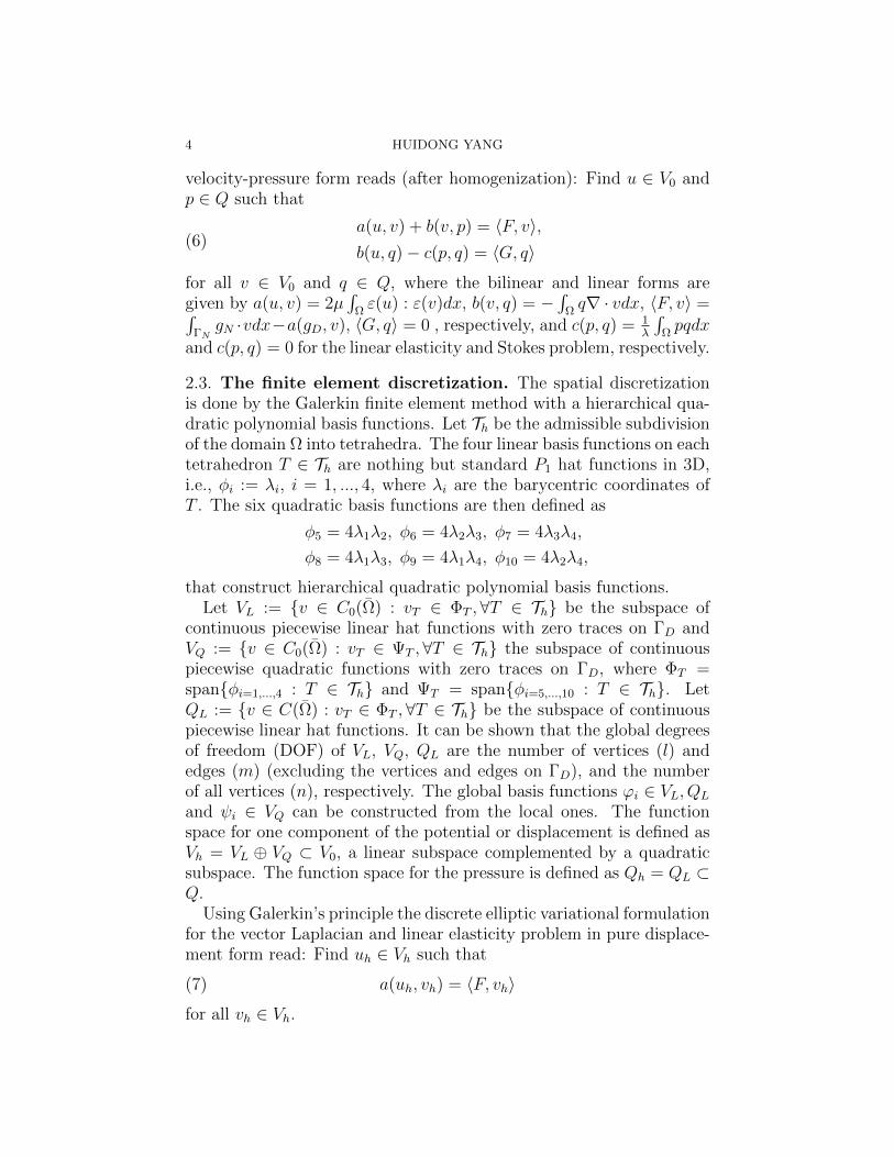
velocity-pressure form reads (after homogenization): Find u ∈ V0 andp ∈ Q such that

(6)a(u, v) + b(v, p) = 〈F, v〉,b(u, q)− c(p, q) = 〈G, q〉

for all v ∈ V0 and q ∈ Q, where the bilinear and linear forms aregiven by a(u, v) = 2µ

∫Ωε(u) : ε(v)dx, b(v, q) = −

∫Ωq∇ · vdx, 〈F, v〉 =∫

ΓNgN ·vdx−a(gD, v), 〈G, q〉 = 0 , respectively, and c(p, q) = 1

λ

∫Ωpqdx

and c(p, q) = 0 for the linear elasticity and Stokes problem, respectively.

2.3. The finite element discretization. The spatial discretizationis done by the Galerkin finite element method with a hierarchical qua-dratic polynomial basis functions. Let Th be the admissible subdivisionof the domain Ω into tetrahedra. The four linear basis functions on eachtetrahedron T ∈ Th are nothing but standard P1 hat functions in 3D,i.e., φi := λi, i = 1, ..., 4, where λi are the barycentric coordinates ofT . The six quadratic basis functions are then defined as

φ5 = 4λ1λ2, φ6 = 4λ2λ3, φ7 = 4λ3λ4,

φ8 = 4λ1λ3, φ9 = 4λ1λ4, φ10 = 4λ2λ4,

that construct hierarchical quadratic polynomial basis functions.Let VL := v ∈ C0(Ω) : vT ∈ ΦT , ∀T ∈ Th be the subspace of

continuous piecewise linear hat functions with zero traces on ΓD andVQ := v ∈ C0(Ω) : vT ∈ ΨT ,∀T ∈ Th the subspace of continuouspiecewise quadratic functions with zero traces on ΓD, where ΦT =spanφi=1,...,4 : T ∈ Th and ΨT = spanφi=5,...,10 : T ∈ Th. LetQL := v ∈ C(Ω) : vT ∈ ΦT ,∀T ∈ Th be the subspace of continuouspiecewise linear hat functions. It can be shown that the global degreesof freedom (DOF) of VL, VQ, QL are the number of vertices (l) andedges (m) (excluding the vertices and edges on ΓD), and the numberof all vertices (n), respectively. The global basis functions ϕi ∈ VL, QL

and ψi ∈ VQ can be constructed from the local ones. The functionspace for one component of the potential or displacement is defined asVh = VL ⊕ VQ ⊂ V0, a linear subspace complemented by a quadraticsubspace. The function space for the pressure is defined as Qh = QL ⊂Q.

Using Galerkin’s principle the discrete elliptic variational formulationfor the vector Laplacian and linear elasticity problem in pure displace-ment form read: Find uh ∈ Vh such that

(7) a(uh, vh) = 〈F, vh〉

for all vh ∈ Vh.


The discrete mixed variational formulation for the elasticity problemin mixed displacement-pressure form and the Stokes problem in mixedvelocity-pressure form reads: Find (uh, ph) ∈ Vh ×Qh such that

(8)a(uh, vh) + b(vh, ph) = 〈F, vh〉,b(uh, qh)− c(ph, qh) = 〈G, qh〉

for all vh ∈ Vh and qh ∈ Qh.The finite element solutions uh ∈ Vh and ph ∈ Qh are expressed by

the ansatz:

uh = ulh + uqh =l∑

i=1

uliϕi +m∑i=1

uqiψi, ph =n∑i=1

pliϕi,

respectively, where uli, uqi ∈ R3 and pli ∈ R. It is easy to see the finite

element solution uh is the sum of the linear and quadratic part, ulhand uqh, respectively. For the pressure ph, we have a linear approxima-tion. The mixed finite element for the elasticity and Stokes problemis classical Taylor-Hood element, that fulfills the inf − sup stability re-quirement; see, e.g., [6].

2.4. SPD and saddle point linear systems of equations. Usingthe finite element discretization (including homogenization), we obtainthe following symmetric and positive definite (SPD) system of equa-tions for the elliptic problem:

(9) Au =

[Kll KT

ql

Kql Kqq

] [uluq

]=

[fl

fq

]= f,

where Kll = (a(ϕi, ϕj)), Kql = a(ϕj, ψi), Kqq = a(ψi, ψj), ul = (uli),uq = (uqi ), f l = (〈F, ϕi〉) and f

q= (〈F, ψi〉).

For the elasticity problem in mixed displacement-pressure form andthe Stokes problem in mixed velocity-pressure form, we obtain the fol-lowing symmetric indefinite system of equations:(10)[

A BT

B −C

]︸︷︷︸

=:K

[up

]=

Kll KTql BT

ll

Kql Kqq BTlq

Bll Blq −Cll

uluqpl

=

fl

fq

gl

=

[fg

]

where Kll = (a(ϕi, ϕj)), Kql = a(ϕj, ψi), Kqq = a(ψi, ψj), Bll =b(ϕi, ϕj), Blq = b(ϕi, ψj), Cll = c(ϕi, ϕh), ul = (uli), uq = (uqi ),

pl

= (pli), f l = (〈F, ϕi〉), f q = (〈F, ψi〉) and gl

= (〈G,ϕi〉). It is

obvious that for the Stokes problem, C = 0.

6 HUIDONG YANG

In the following, we focus on how to solve the above two systems ofequations (9) and (10) using an algebraic multigrid method.

3. An algebraic multigrid method

3.1. The basic algebraic multigrid iteration. The basic AMG it-eration applied to a general linear system of equations Kx = b is givenin Algorithm 1, with mpre and mpost being the number of pre- and post-smoothing steps (steps 1-3 and 14-16, respectively). By choosing ν = 1and ν = 2, the iterations in Algorithm 1 are called V- and W-cycle, re-spectively. As a convention, we use l = 0, ..., L to indicate the algebraicmultigrid levels from the finest level l = 0 to the coarsest level l = L.On the coarsest level L, the system is solved by any direct solver (step6). The coarse grid correction step is indicated in steps 4-13. The fullAMG iterations are realized by repeated application of this algorithm.The iteration in this algorithm is also combined with the Krylov sub-space methods, that usually leads to accelerated convergence of V-cycleor W-cycle preconditioned methods [22].

Algorithm 1 Basic AMG iteration: AMG(Kl, xl, bl)

1: for k = 1 to mpre do2: xk+1

l = Sl(xkl , bl)3: end for4: bl+1 = Rl+1

l (bl −Klxl),5: if l+1=L then6: Solve KLxL = bL7: else8: xl+1 = 0,9: for k = 1, ..., ν do

10: xl+1 =AMG(Kl+1, xl+1, bl+1),11: end for12: end if13: xl = xl + P l

l+1xl+1,14: for k = 1 to mpost do15: xk+1

l = Sl(xkl , bl),16: end for17: return xl.

3.2. A new heuristic coarsening strategy.


3.2.1. Case I : The SPD system. A robust coarsening strategy is animportant feature of the AMG method, that is used to construct thesystem matrices on coarse levels l = 1, 2, ..., L. For the second orderelliptic equations discretized by low order finite element or boundaryelement methods, some well known graph-based black-box or grey-box type AMG methods have been introduced and applied, see, e.g.,[3, 11, 17, 13, 12]. The general strategy is to split the nodes into the setsof coarse and fine nodes, based on the graph connectivity of the systemmatrix or the constructed auxiliary matrix (”virtual” finite elementmesh [17]).

When applying such a technique to the system matrix in (9), weobtain a very dense graph connectivity constructed from the stiffnessmatrix A, that contains connectivities for the linear DOF, the quadraticDOF and the coupling between them. This will lead to a mixture ofdifferent oder of DOF and may cause additional difficulty to constructthe interpolation operators. In fact, from our numerical studies, weobserve the loss of optimality of the AMG method when such a densegraph connectivity is adopted for coarse system matrix construction.Therefore, we construct the graph connectivities only for the linear andquadratic DOF, i.e., for Kll and Kqq, respectively. We simply neglectthe coupling connectivity in Kql. By this means, we avoid the mixtureof different order of DOF on the coarse level. In addition, we are ableto construct and control the interpolation operators for the linear andquadratic part, respectively. A simple comparison of the classical andnew graph connectivities is illustrated in Fig. 1.

Figure 1. Graph connectivity constructed using thenew (left) and the classical (right) strategies: linear DOF(solid line) , quadratic DOF (dashed line) , coupling(dashed dot lines).

8 HUIDONG YANG

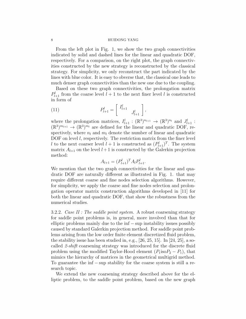
From the left plot in Fig. 1, we show the two graph connectivitiesindicated by solid and dashed lines for the linear and quadratic DOF,respectively. For a comparison, on the right plot, the graph connectiv-ities constructed by the new strategy is reconstructed by the classicalstrategy. For simplicity, we only reconstruct the part indicated by thelines with blue color. It is easy to obverse that, the classical one leads tomuch denser graph connectivities than the new one due to the coupling.

Based on these two graph connectivities, the prolongation matrixP ll+1 from the coarse level l + 1 to the next finer level l is constructed

in form of

(11) P ll+1 =

[I ll+1

J ll+1

],

where the prolongation matrices, I ll+1 : (R3)nl+1 → (R3)nl and J ll+1 :(R3)ml+1 → (R3)ml are defined for the linear and quadratic DOF, re-spectively, where nl and ml denote the number of linear and quadraticDOF on level l, respectively. The restriction matrix from the finer levell to the next coarser level l + 1 is constructed as (P l

l+1)T . The systemmatrix Al+1 on the level l+1 is constructed by the Galerkin projectionmethod:

Al+1 = (P ll+1)TAlP

ll+1.

We mention that the two graph connectivities for the linear and qua-dratic DOF are naturally different as illustrated in Fig. 1. that mayrequire different coarse and fine nodes selection algorithms. However,for simplicity, we apply the coarse and fine nodes selection and prolon-gation operator matrix construction algorithms developed in [11] forboth the linear and quadratic DOF, that show the robustness from thenumerical studies.

3.2.2. Case II : The saddle point system. A robust coarsening strategyfor saddle point problems is, in general, more involved than that forelliptic problems mainly due to the inf − sup instability issues possiblycaused by standard Galerkin projection method. For saddle point prob-lems arising from the low order finite element discretized fluid problem,the stability issue has been studied in, e.g., [26, 25, 15]. In [24, 25], a so-called 2-shift coarsening strategy was introduced for the discrete fluidproblem using the modified Taylor-Hood element (P1isoP2 − P1), thatmimics the hierarchy of matrices in the geometrical multigrid method.To guarantee the inf − sup stability for the coarse system is still a re-search topic.

We extend the new coarsening strategy described above for the el-liptic problem, to the saddle point problem, based on the new graph


connectivity construction. As illustrated in Fig. 2, we show the graphconnectivities constructed for the velocity (displacement) and pressure.For the velocity, we follow the same strategy as for the SPD system; seethe left plot. For the pressure, we have conventional graph connectivityfor the linear finite element matrix; see the right plot.

Figure 2. Graph connectivities constructed using thenew strategies for velocity (displacement) (left) and pres-sure (right).

Based on the graph connectivities, the prolongation matrix P ll+1 from

the coarse level l + 1 to the next finer level l is constructed in form of

(12) P ll+1 =

I ll+1

J ll+1

H ll+1

,where the prolongation matrices, I ll+1 : (R3)nl+1 → (R3)nl and J ll+1 :(R3)ml+1 → (R3)ml are defined for the linear and quadratic velocityDOF, respectively, where nl and ml denote the number of linear andquadratic velocity DOF on level l, respectively, H l

l+1 : Rkl+1 → Rkl forthe pressure DOF, where kl the number of pressure DOF on level l.The restriction matrix from the finer level l to the next coarser levell + 1 is constructed as (P l

l+1)T . The system matrix Kl+1 on the levell + 1 is constructed by the Galerkin projection method:

Kl+1 = (P ll+1)TKlP

ll+1.

We admit that the inf − sup stability of the coarse system is still openby this construction. However, from the numerical studies, we observequite satisfactory results using this new coarsening strategy. Neverthe-less, we are at least able to obtain efficient multigrid preconditionersby using pure Galerkin projection; see comments in, e.g., [21, 27] and

10 HUIDONG YANG

numerical experiments for the Stokes problem using the low order finiteelement discretization in, e.g., [10].

3.3. The smoothing procedure. To complete the algebraic multi-grid algorithm, a smoothing procedure is needed. As conventionalchoices, we employ the damped block Jacobi and block Gauss-Seidelsmoothers for the SPD system (9), that are widely used in the multi-grid methods. For the saddle point system (10), we have consideredthe following smoothers, that were originally designed and analyzed inthe GMG method.

3.3.1. The multiplicative Vanka smoother. The multiplicative Vankasmoother was introduced in [23] for the fluid problem. We have recentlydeveloped an AMG method with this smoother for solving the nonlinearand nearly incompressible hyperelastic models in fluid-structure inter-action simulation [14]. To adapt this smoother for the Taylor-Hoodelement, we first construct the patches Pi, i = 1, ..., n. Each patchcontains one pressure DOF, and the connected linear and quadraticvelocity DOF indicated by the connectivity of matrices Bll and Blq,respectively. A typical patch Pi is illustrated in Fig. 3.

pressure DOF

linear velocity DOF

quadratic velocity DOF

Figure 3. A typical local patch Pi for the Taylor-Hoodelement contains one pressure DOF, and connected linearand quadratic velocity DOF.


The local (correction) problem on Pi is extracted by a canonicalprojection of the global one (10) to local one on Pi:

(13)

[uk+1i

pk+1i

]=

[ukipki

]+ ω

[Ai BT

i

Bi −Ci

]−1 [rku,irkp,i

]with k representing the smoothing step and ω being a damping pa-rameter. Here [(rku,i)

T , (rkp,i)T ]T denotes the residual updated in a mul-

tiplicative manner. As we observe from the numerical studies, thissmoother shows the efficiency and robustness if it is used in the AMGpreconditioner but not in the stand-alone AMG solver.

3.3.2. The Braess-Sarazin-type smoother. This smoother was introducedin [5] and approximated in [30], that has been applied to the fluid prob-lem [25, 26], the nearly incompressible elasticity problem [28] and thefluid-structure interaction problem [29]. One smoothing step corre-sponds to a preconditioned Richardson method:

(14)

[uk+1

pk+1

]=

[uk

pk

]+ K−1

[f − Auk −BTpk

g −Buk + Cpk

]with preconditioner

(15) K =

[A BT

B BA−1BT − S

].

As in [24], we use A = 2D, where D represents the diagonal of A. We

use an AMG preconditioner S for the approximated Schur complementC +BA−1B.

3.3.3. The segregated Gauss-Seidel smoother. This smoother was veryrecently introduced in [7] as a segregated Gauss-Seidel smoother basedon a Uzawa-type iteration. Such a Uzawa method (see, e.g., [2]) canbe reinterpreted as a preconditioned Richardson method:

(16)

[uk+1

pk+1

]=

[uk

pk

]+ K−1

[f − Auk −BTpk

g −Buk + Cpk

]with the preconditioner

(17) K =

[AB −ω−1I

],

where ω is a properly chosen parameter, A is a (e.g., AMG) precon-ditioner for A. However, to get a multigrid smoother, this is relaxedby choosing some proper smoother MA for A instead of a precondi-tioner A; see [7]. The theoretical analysis requirement for MA has beenspecified therein. In our setting, we have chosen MA as a damped

12 HUIDONG YANG

block Jacobi smoother with a damping parameter 0.5. Compared tothe Braess-Sarazin-type smoother, this smoother avoids the expliciteconstruction of the approximate Schur complement.

4. Numerical results

4.1. Meshes, boundary conditions and coarsening for the vec-tor Laplacian and linear elasticity problems. We consider a unitcube (0, 1)3 as the computational domain for the vector Laplacian andlinear elasticity problems. The domain is subdivided into tetrahedrawith four levels of mesh refinement L1 − L4. The number of tetrahe-dron (#Tet), nodes (#Nodes) and midside nodes (#Midside nodes),and the total number of DOF for elliptic ( #DOF (elliptic) ) and sad-dle point ((#DOF (saddle point)) systems are shown in Table 1. We

Level L1 L2 L3 L4

#Tet 64 512 4096 32768#Nodes 125 729 4913 35937

#Midside nodes 604 4184 31024 238688#DOF (elliptic) 2187 14739 107811 823875

#DOF (saddle point) 2312 15468 112724 859812

Table 1. Number of tetrahedron (#Tet) , nodes(#Nodes), Midside nodes (#Midside nodes), and totalnumber of DOF for elliptic ( #DOF (elliptic) ) and sad-dle point (#DOF (saddle point)) systems on four levelsL1 − L4.

fix the bottom of the domain, i.e., u = [0, 0, 0]T at z = 0, prescribe aDirichlet data on the top, i.e., u = [0, 0, 1]T at z = 1, and use zero Neu-mann condition on the rest of the boundaries. For the linear elasticityproblem, we set µ = 1.15e+ 06 and λ = 1.73e+ 06. In Fig. 4, we plotthe value of ‖u‖R3 of the numerical solution u (indicated by the color)for the vector Laplacian (left) and the linear elasticity problem in puredisplacement form (right), respectively. For visualization purpose, weplot the vector fields of potential and deformation, that is scaled by afactor of 0.1.

As a comparison, on each algebraically coarsening level, we show thenumber of linear and quadratic DOF (# Linear DOF and # QuadraticDOF, respectively) in the new coarsening strategy, and the classicalcoarsening strategy (# Non-separating DOF); see in Table 2 the num-ber of DOF on each coarsening level for the vector Laplacian and linear


Figure 4. Numerical results of the vector Laplacian(left) and linear elasticity (right) problem.

elasticity problem on the level L4. It is obvious to see these two strate-gies lead to different graph connectivity in the coarsening procedure.

Coarsening Levels 0 1 2 3 4#Linear DOF 107811 14739 2187 375 81

#Quadratic DOF 716064 104544 6366 369 39#Non-separating DOF 823875 88467 2187 375 24

Table 2. Number of linear and quadratic DOF in thenew coarsening strategy, and the total DOF in the non-separating coarsening strategy at level L4, for the vectorLaplacian and linear elasticity problems.

4.2. Numerical performance for the vector Laplacian prob-lem. Before showing the AMG performance with the new coarsen-ing strategy, we demonstrate the performance with a black-box typeAMG [11] in Table 3 for the vector Laplacian problem, where non-separating coarsening strategy is used. For both AMG and AMGpreconditioned CG methods, we use the relative residual error ‖f −Auk‖l2/‖f − Au0‖l2 = 1.0e − 11 in the l2−norm as stopping criteria,where k denotes the number of AMG iterations. In each iteration ofthe AMG solver, we use 2 W-cycles and 1 pre- and post-smoothingstep. As observed, the AMG and the AMG preconditioned CG are not

14 HUIDONG YANG

robust with respect to the mesh refinement, i.e., the iteration numberincreases with mesh refinement.

Levels L1 L2 L3 L4

#It AMG 90 158 > 200 > 200#It PCG AMG 22 25 36 64

Table 3. Performance of black-box type AMG solver(#It AMG) and AMG preconditioned conjugate gradientsolver (#It PCG AMG) for the vector Laplacian prob-lem.

Now we show the performance of the AMG and AMG precondi-tioned CG solvers using the new coarsening strategy. Note, that inthe following numerical tests, we stop the iterations when the relativeresidual error in the l2−norm is reduced by a factor 1011. We considerthe Jacobi smoother with damping parameter 0.5 and 1 or 2 pre- andpost-smoothing steps (JA-1-1-0.5 or JA-2-2-0.5), and the Gauss-Seidelsmoother with 1 or 2 pre- and post-smoothing steps (GS-1-1 or GS-2-2). In Table 4, we show the performance of the AMG solver for thevector Laplacian problem using V-cycle with different smoothers. InTable 5, we show the performance using W-cycle. In Table 6 and 7, weshow the performance of the AMG preconditioned CG using V- andW-cycles with different smoothers, respectively.

As observed, the iterations for each solver are independent of meshrefinement levels. The AMG solver using the Gauss-Seidel smoothershows better performance than the damped Jacobi smoother. By usingthe CG acceleration, we observe similar performance with two differ-ent smoothers. In addition, we observe, that the V- and W-cyclesdemonstrate almost the same performance. We also observe that thecomputational cost is proportional to the number of DOF.

Level L1 L2 L3 L4

#It ( JA-1-1-0.5 ) 129 125 124 128#It ( JA-2-2-0.5 ) 65 65 65 66

#It ( GS-1-1 ) 43 46 47 47#It ( GS-2-2 ) 23 24 24 24

Table 4. Performance of the AMG solver for thevector Laplacian problem using V-cycle with differentsmoothers.


Level L1 L2 L3 L4

#It ( JA-1-1-0.5 ) 128 124 121 123#It ( JA-2-2-0.5 ) 65 64 63 64

#It ( GS-1-1 ) 43 46 47 47#It ( GS-2-2 ) 23 24 24 24

Table 5. Performance of the AMG solver for thevector Laplacian problem using W-cycle with differentsmoothers.

Level L1 L2 L3 L4

#It ( JA-1-1-0.5 ) 30 30 30 30#It ( JA-2-2-0.5 ) 21 22 22 22

#It ( GS-1-1 ) 26 29 29 30#It ( GS-2-2 ) 17 19 19 19

Table 6. Performance of the AMG preconditioned CGsolver for the vector Laplacian problem using V-cyclewith different smoothers.

Level L1 L2 L3 L4

#It ( JA-1-1-0.5 ) 30 30 30 29#It ( JA-2-2-0.5 ) 21 21 21 21

#It ( GS-1-1 ) 26 29 29 29#It ( GS-2-2 ) 17 18 18 18

Table 7. Performance of the AMG preconditioned CGsolver for the vector Laplacian problem using W-cyclewith different smoothers.

4.3. Numerical performance for the linear elasticity problemin pure displacement form. We perform the same test for the lin-ear elasticity problem. In Table 8, we show the performance of theAMG solver for the linear elasticity problem using V-cycle with differ-ent smoothers. In Table 9, we show the performance using W-cycle. InTable 10 and 11, we show the performance of the AMG preconditionedCG using V- and W-cycles with different smoothers, respectively.

As observed, the damped Jacobi smoother does not work for thistest problem. The AMG solver using the Gauss-Seidel smoother showsgood performance. By using the CG acceleration, we observe improved

16 HUIDONG YANG

performance. We observe, that the V- and W-cycles demonstrate al-most the same performance.

Level L1 L2 L3 L4

#It ( JA-1-1-0.5 ) − − − −#It ( JA-2-2-0.5 ) − − − −

#It ( GS-1-1 ) 80 78 76 75#It ( GS-2-2 ) 44 40 39 39

Table 8. Performance of the AMG solver for the linearelasticity problem in pure displacement form using V-cycle with different smoothers..

Level L1 L2 L3 L4

#It ( JA-1-1-0.5 ) − − − −#It ( JA-2-2-0.5 ) − − − −

#It ( GS-1-1 ) 80 78 75 73#It ( GS-2-2 ) 44 40 39 44

Table 9. Performance of the AMG solver for the linearelasticity problem in pure displacement form using W-cycle with different smoothers..

Level L1 L2 L3 L4

#It ( JA-1-1-0.5 ) 50 81 − −#It ( JA-2-2-0.5 ) 32 63 − −

#It ( GS-1-1 ) 40 43 43 42#It ( GS-2-2 ) 28 27 27 27

Table 10. Performance of the AMG preconditioned CGsolver for the linear elasticity problem in pure displace-ment form using V-cycle with different smoothers.

4.4. Numerical performance for linear elasticity problem inmixed form. For the linear elasticity problem in mixed displacement-pressure form, we plot the simulation results of the displacement andpressure on the left and right plots of Fig. 5, respectively.

We set the relative residual error 1.0e−09 in the corresponding normas stopping criteria for solving the saddle point system (indefinite) with


Level L1 L2 L3 L4

#It ( JA-1-1-0.5 ) 47 80 − −#It ( JA-2-2-0.5 ) 32 62 − −

#It ( GS-1-1 ) 39 44 42 41#It ( GS-2-2 ) 28 27 27 26

Table 11. Performance of the AMG preconditioned CGsolver for the linear elasticity problem in pure displace-ment form using W-cycle with different smoothers.

Figure 5. Numerical results of the displacement (left)and pressure (right) for the linear elasticity problem inmixed form.

both the AMG solver and AMG preconditioned GMRES (see [19])method. We will only consider the V-cyle for the remaining tests.

The AMG solver with the Vanka smoother does not show the ro-bustness and efficiency in this case. However combined with GMRESacceleration, the V-cycle preconditioner with such a smoother showsimproved performance. We observe acceptable performance of one ortwo V-cycles (1 V-cycle or 2 V-cycle) preconditioned GMRES solver inTable 12. In each cycle, we use only one pre- and post-smoothing step.

The Braess-Sarazin smoother shows better performance. We observethe robustness with respect to the mesh size of the AMG solver andV-cycle preconditioned GMRES solver using such a smoother; see it-eration numbers of the AMG solver using one or two Braess-Sarazinsmoothing steps (Braess-Sarazin-1-1 or Braess-Sarazin-2-2) in Table

18 HUIDONG YANG

Level L1 L2 L3 L4

#It ( 1 V-cycle ) 60 45 49 69#It ( 2 V-cycles ) 42 30 32 45

Table 12. Performance of the V-cycle preconditionedGMRES solver for the linear elasticity problem in mixedform using one pre/poster Vanka smoother.

13, and one or two V-cycles (1 V-cycle or 2 V-cycle) preconditionedGMRES solver in Table 14, respectively.

Level L1 L2 L3 L4

#It ( Braess-Sarazin-1-1 ) 135 133 125 117#It ( Braess-Sarazin-2-2 ) 71 70 66 62

Table 13. Performance of the AMG solver for the linearelasticity problem in mixed form using the V-cycle withthe Braess-Sarazin smoother.

Level L1 L2 L3 L4


Table 14. Performance of the V-cycle preconditionedGMRES solver for the linear elasticity problem in mixedform using one pre/post Braess-Sarazin smoother.

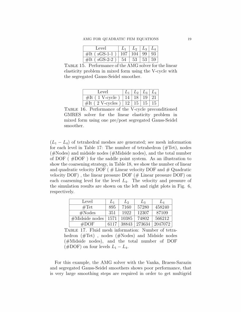
Using the segregated Gauss-Seidel smoother (sGS), we observe goodperformance. For all tests, we use ω = 0.125. The robustness with re-spect to the mesh size of the AMG solver can be observed; see iterationnumbers of the AMG solver using one or two segregated Gauss-Seidelsmoothing steps (sGS-1-1 or sGS-2-2) in Table 15. The efficiency is fur-ther improved when combined with the Krylov subspace acceleration;see iteration numbers of one or two V-cycles (1 V-cycle or 2 V-cycle)preconditioned GMRES solver in Table 16.

4.5. Numerical performance for the Stokes problem. The com-putational domain for the Stokes problem is prescribed by an insideof a cylinder, that has radius of 1 with center point (0, 0, 0) on theinflow boundary (where u = (1.0, 0, 0)), and center point (10, 0, 0) onthe outflow boundary (where (2µε(u) − pI)n = (0, 0, 0)). On the restof the boundaries u = (0, 0, 0). For all tests, we set µ = 0.5. Four levels


Level L1 L2 L3 L4

#It ( sGS-1-1 ) 107 104 99 93#It ( sGS-2-2 ) 54 53 53 59

Table 15. Performance of the AMG solver for the linearelasticity problem in mixed form using the V-cycle withthe segregated Gauss-Seidel smoother.

Level L1 L2 L3 L4


Table 16. Performance of the V-cycle preconditionedGMRES solver for the linear elasticity problem inmixed form using one pre/post segregated Gauss-Seidelsmoother.

(L1 − L4) of tetrahedral meshes are generated; see mesh informationfor each level in Table 17: The number of tetrahedron (#Tet), nodes(#Nodes) and midside nodes (#Midside nodes), and the total numberof DOF ( #DOF ) for the saddle point system. As an illustration toshow the coarsening strategy, in Table 18, we show the number of linearand quadratic velocity DOF ( # Linear velocity DOF and # Quadraticvelocity DOF) , the linear pressure DOF (# Linear pressure DOF) oneach coarsening level for the level L4. The velocity and pressure ofthe simulation results are shown on the left and right plots in Fig. 6,respectively.

Level L1 L2 L3 L4

#Tet 895 7160 57280 458240#Nodes 351 1922 12307 87109

#Midside nodes 1571 10385 74802 566212#DOF 6117 38843 273634 2047072

Table 17. Fluid mesh information: Number of tetra-hedron (#Tet) , nodes (#Nodes) and Midside nodes(#Midside nodes), and the total number of DOF(#DOF) on four levels L1 − L4.

For this example, the AMG solver with the Vanka, Braess-Sarazinand segregated Gauss-Seidel smoothers shows poor performance, thatis very large smoothing steps are required in order to get multigrid

20 HUIDONG YANG

Coarsening Levels 0 1 2 3 4#Linear velocity DOF 261327 36921 5766 1053 267

#Quadratic velocity DOF 1698636 213492 14142 1053 93#Linear pressure DOF 87109 12307 1922 351 89

Table 18. Number of linear and quadratic velocity, andlinear pressure DOF in the new coarsening strategy atlevel L4 for the Stokes problem.

Figure 6. Numerical results of the Stokes velocity (left)and pressure (right).

convergence rate. However, this will lead to very expensive computa-tional cost. In addition, we observe unsatisfactory performance of theAMG preconditioned Krylov subspace method using the V-cycle withthe Vanka and segregated Gauss-Seidel smoothers. Therefore, we onlyreport the performance of the AMG preconditioned GMRES solver us-ing the Braess-Sarazin smoother, that is shown in Table 19. We setrelative residual error 1.0e− 09 in the corresponding norm as stoppingcriteria of the AMG preconditioned GMRES solver. It is easy to see,with the Krylov subspace acceleration, the performance is greatly im-proved, using one or two V-cycle (1 V-cycle or 2 V-cycle) preconditionerwith one pre- and post-smoothing steps.


Level L1 L2 L3 L4


Table 19. Performance of the V-cycle preconditionedGMRES solver for the Stokes problem using one pre/postBraess-Sarazin smoother.

5. Conclusions

In this work, we have developed an AMG method used as a stand-alone solver or preconditioner in the Krylov subspace methods for solv-ing the finite element equations of the vector Laplacian problem, lin-ear elasticity problem in pure displacement and mixed displacement-pressure form, and the Stokes problem in mixed velocity-pressure formin 3D. We have developed a new strategy to construct the hierarchy ofthe AMG coarsening system using the hierarchical quadratic basis func-tions. The numerical studies have demonstrated the good performanceof the AMG solvers or the AMG preconditioned Krylov subspace meth-ods for the elliptic and saddle point systems, respectively. In particular,the AMG preconditioned Krylov subspace methods show much betterrobustness and efficiency for solving both systems compared with theAMG stand-alone solvers. From this point of view, the AMG methoddeveloped in this work can be used as a robust and efficient solver orpreconditioner for the SPD system and the saddle point system withcompressible materials, and as a robust and efficient preconditionerfor the saddle point system with incompressible materials. It is alsopossible to extend this AMG method for high-order hierarchical finiteelement basis functions.

Acknowledgement

The author would like to thank Prof. Ulrich Langer for his encour-agement and many enlightened discussions on this work.

References

[1] R.A. Adams and J.J.F. Fournier. Sobolev Spaces. Academic Press, Amsterdam,Boston, 2003.

[2] Michele Benzi, G.H. Golub, and J. Liesen. Numerical solution of saddle pointproblems. Acta Numerica, 14:1–137, 5 2005.

[3] D. Braess. Towards algebraic multigrid for elliptic problems of second order.Computing, 55(4):379–393, 1995.

[4] D. Braess. Finite Elements - Theory, Fast Solvers, and Applications in SolidMechanics. Cambridge University Press, Cambridge, New York, 2007.

22 HUIDONG YANG

[5] D. Braess and R. Sarazin. An efficient smoother for the Stokes problem. Appl.Numer. Math., 23(1):3–19, 1997.

[6] F. Brezzi and M. Fortin. Mixed and Hybrid Finite Element Methods. Springer,New York, 1991.

[7] F.J. Gaspar, Y. Notay, C.W. Oosterlee, and C. Rodrigo. A simple and efficientsegregated smoother for the discrete Stokes equations. SIAM J. Sci. Comput.,36(3):A1187–A1206, 2014.

[8] G. Haase and U. Langer. Modern Methods in Scientific Computing and Ap-plications, volume 75 of NATO Science Series II. Mathematics, Physics andChemistry, chapter Multigrid Methods: From Geometrical to Algebraic Ver-sions, pages 103–154. Kluwer Academic Press, Dordrecht, 2002.

[9] W. Hackbusch. Multi-Grid Methods and Applications. Springer, Heidelberg,2003.

[10] A. Janka. Smoothed aggregation multigrid for a Stokes problem. Comput. Vi-sual. Sci., 11(3):169–180, 2008.

[11] F. Kickinger. Algebraic multigrid for discrete elliptic second-order problems.In Multigrid Methods V. Proceedings of the 5th European Multigrid conference(ed. by W. Hackbush), Lecture Notes in Computational Sciences and Engineer-ing, vol. 3, pages 157–172. Springer, 1998.

[12] U. Langer and D. Pusch. Data-sparse algebraic multigrid methods for largescale boundary element equations. Appl. Numer. Math., 54(34):406–424, 2005.

[13] U. Langer, D. Pusch, and S. Reitzinger. Efficient preconditioners for boundaryelement matrices based on grey-box algebraic multigrid methods. Int J NumerMeth Engng, 58(13):1937–1953, 2003.

[14] U. Langer and H. Yang. Partitioned solution algorithms for fluid-structureinteraction problems with hyperelastic models. J. Comput. Appl. Math.,276(0):47–61, 2015.

[15] B. Metsch. Algebraic Multigrid (AMG) for Saddle Point Systems. PhD thesis,Rheinischen Friedrich-Wihelms-Universitat Bonn, 2013.

[16] A. Napov and Y. Notay. Algebraic multigrid for moderate order finite elements.SIAM J Sci Comput, 2014. to appear.

[17] S. Reitzinger. Algebraic Multigrid Methods for Large Scale Finite ElementMethods. PhD thesis, Johannes Kepler University Linz, 2001.

[18] J. W. Ruge and K. Stuben. Algebraic multigrid. In S.F. McCormick, editor,Multigrid Methods, volume 3 of Frontiers in Applied Mathematics, pages 73–130. SIAM, Philadelphia, PA, 1987.

[19] Y. Saad and Martin H. Schultz. GMRES: A generalized minimal residual al-gorithm for solving nonsymmetric linear systems. SIAM J. Sci. Stat. Comput.,7(3):856–869, 1986.

[20] S. Shu, D. Sun, and J. Xu. An algebraic multigrid method for higher-orderfinite element discretizations. Computing, 77(4):347–377, 2006.

[21] K. Stuben. Multigrid, chapter Appendix A: An introduction to algebraic multi-grid, pages 413–533. Academic Press, 2001.

[22] K. Stuben. A review of algebraic multigrid. J. Comput. Appl. Math.,128(12):281–309, 2001.

[23] S.P. Vanka. Block-implicit multigrid solution of Navier-Stokes equations inprimitive variables. J. Comput. Phys., 65(1):138–158, 1986.


[24] M. Wabro. Algebraic Multigrid Methods for the Numerical Solution of the In-compressible Navier-Stokes Equations. PhD thesis, Johannes Kepler UniversityLinz, 2003.

[25] M. Wabro. Coupled algebraic multigrid methods for the Oseen problem. Com-put Visual Sci, 7(3-4):141–151, 2004.

[26] M. Wabro. AMGe—coarsening strategies and application to the Oseen equa-tions. SIAM J Sci Comput, 27(6):2077–2097, 2006.

[27] T. Wiesner. Flexible Aggregration-based Algebraic Multigrid Method for Con-tact and Flow Problems. PhD thesis, Technischen Universitat Munchen, 2015.

[28] H. Yang. Partitioned solvers for the fluid-structure interaction problems witha nearly incompressible elasticity model. Comput. Visual. Sci., 14(5):227–247,2011.

[29] H. Yang and W. Zulehner. Numerical simulation of fluid-structure interactionproblems on hybrid meshes with algebraic multigrid methods. J. Comput. Appl.Math., 235(18):5367–5379, 2011.

[30] W. Zulehner. A class of smoothers for saddle point problems. Computing,65(3):227–246, 2000.

Johann Radon Institute for Computational and Applied Mathemat-ics (RICAM), Austrian Academy of Sciences, Altenberger Strasse 69,A-4040 Linz, Austria

E-mail address: [email protected]

an algebraic multigrid method for - arxiv · an algebraic multigrid method for quadratic finite...

Documents