An Adaptive Computational Network Modelfor Strange Loops in Political Evolution

in Society

Julia Anten1, Jordan Earle1, and Jan Treur2(&)

1 Computational Science, University of Amsterdam,Amsterdam, The Netherlands

juliaanten@hotmail.com, jordanalexearle@gmail.com2 Social AI Group, Vrije Universiteit Amsterdam, Amsterdam, The Netherlands

j.treur@vu.nl

Abstract. In this paper a multi-order adaptive temporal-causal network modelis introduced to model political evolution. The computational network modelmakes use of Hofstadter’s notion of a Strange Loop and was tested and validatedsuccessfully to reflect political oscillations seen in presidential elections in theUSA over time.

1 Introduction

Hofstadter [7] originally described a Strange Loop as a phenomenon that, after goingthrough a hierarchy of levels, you would return to the starting level; see also [8, 9]. Inhis original literature, Holfstadter illustrates this for common domains such as graphicalart (Escher), music (Bach), and logical paradoxes (Gödel) [12, 15]. Holfstadter theo-rised that the brain may also use Strange Loops in the creation of human intelligenceand consciousness. Although at a conceptual level much literature can be foundreferring to Strange Loops in one way or the other, almost none of it actually shows acomputational model for this phenomenon. An exception is [19], Ch. 8, where theconcept of multi-order adaptive reified temporal-causal network is exploited to showsome small toy examples of computational Strange Loop models.

In the current paper a more serious and more complex domain is addressed, namelyof political evolution over time. A Strange Loop temporal-causal network was created,tested and validated to reflect political oscillations seen in presidential elections in theUS. The temporal-causal network breaks a political system into 3 groups, the individualpeople, the politicians, and the laws. The individuals’ combined unhappiness causesthem to vote for politicians who align with their desires. The elected politicians in turnvote for the laws which they are aligned to. These laws then cause an effect on theindividuals in the form of the weight for their unhappiness, which then begins the cycleagain.

Once the network design was created, the parameters of the network were varied inorder to obtain oscillations as predicted in empirical Social Science literature. Simu-lation were conducted for the model, changing the initial values of the individuals ofthe poor and rich groups to see if the predicted effects concerning different types of

© Springer Nature Switzerland AG 2020V. V. Krzhizhanovskaya et al. (Eds.): ICCS 2020, LNCS 12138, pp. 604–617, 2020.https://doi.org/10.1007/978-3-030-50417-5_45

laws were seen. The model was then tuned for specific empirical data from the popularvotes from the USA elections over time. All these will be discussed in subsequentsections. Finally, the next steps for the network and an enhancement to the network tocreate an infinite reified network will be discussed.

2 Background: Domain Description

Since [7] many have applied this to various application areas such as advertising [6],self-representation in consciousness [10] and psychotherapeutic understanding [10,17]. However, in this literature no computational models are proposed. After seeinghow the brain and advertising might be modeled in such a loop, the idea to model apolitical system with a strange loop was considered. The original idea was that peoplehave to follow laws, which are created by politicians, who are elected by the people.When considering this system, it can clearly be seen that there is a loop in the levels.The causal pathways affecting people’s lives are affected by the laws, which are createdby causal pathways for politicians; so, people are in effect indirectly voting for theselaws by voting for politicians. Therefore, a literature review was conducted to deter-mine if this observation had been made before and if any models of it existed.

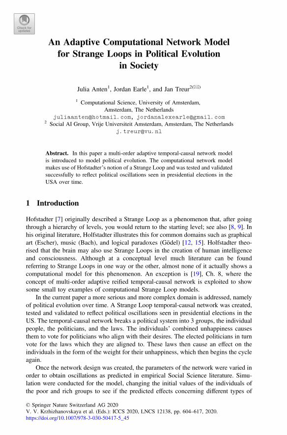
The idea to create a Strange Loop out of a political system is based on observationsmade in the USA political system. The system in the USA can be seen to switchbetween Democratic and Republican leadership every few elections. This switching ofpower has caused the policy on a national and state level change over time, such aswith abortion law and financial policy. The same kind of oscillations have beenobserved in England and in coalitions during war. This type of behavior has been notedas early as 1898, where Lowell [11] observed oscillations in elections in the USA. Itwas, and still is, easily observed when viewing the elections in the USA over time, asseen in Fig. 1 from the above paper.

The second type of feedback she references is the ability of state capacities totransform over time. “State capacities” refers to the ability of the states to implement

Fig. 1. Voting in New York between 1870 and 1897. The number of republicans is shownbelow the black lines, while the number of democrats is shown above. Expected values for theseelections are shown by the dotted line. Adopted from [11].

An Adaptive Computational Network Model 605

and enforce their laws. She writes that “policies transform or expand the capacities ofthe state. They therefore change the administrative possibilities for initiatives in thefuture, and affect later prospects for policy implementation”. This can be seen as theeffect that the laws have on the political structures. This second influence was con-sidered for implementation in this model, but was disregarded as this first model waskept to its basic form to show that the theory was sound.

Pierson [13] notes that “politics produce politics”, discussing how the policy affectsits own creation and upkeep. He states that it has been “increasingly harder to deny thatthat public policies were not only outputs of but important inputs into the politicalprocess”. He notes that interest groups often follow rather than proceed the adoption ofpublic policy, referencing that Skocpol [14] identifies changes in “social groups andtheir political goals and capability” as one of the two major types of political feedback.This can be seen as the political power of the people affecting the laws that governthem, which is the centerpiece of the network which is introduced in the current paper.

More evidence of this phenomenon has been noted more recently by Baumgartnerand Jones [1]. They noted that american policy is characterized by contrasting char-acteristics of stability and dramatic changes which can be expressed in positive andnegative feedback loops. These loops can be seen between the politics and the indi-viduals, leading to more support for this form of conceptualisation.

3 The Adaptive Network Modeling Approach Used

The adaptive computational model is based on the Network-Oriented Modellingapproach based on reified temporal-causal networks described in [18, 19]. The networkstructure characteristics used are as follows. A full specification of a network modelprovides a complete overview of their values in socalled role matrix format.

• Connectivity: The strength of a connection from state X to Y is represented byweight xX,Y

• Aggregation: The aggregation of multiple impacts on state Y by combinationfunction cY(..).

• Timing: The timing of the effect of the impact on state Y by speed factor ηY

Given initial values for the states, these network characteristics fully define thedynamics of the network. For each state Y, its (real number) value at time point t isdenoted by Y(t). Each of the network structure characteristics can be made adaptive byadding extra states for them to the network, called reification states [19]: states WX,Y

for xX,Y, states CY for cY(..), and states HY for ηY. Such reification states get their ownnetwork structure characteristics to define their (adaptive) dynamics and are depicted ina higher level plane, as shown in Fig. 2. For example, using this, the adaptationprinciple called Hebbian learning [5], considered as a form of plasticity of the brain incognitive neuroscience (“neurons that fire together, wire together”) can be modeled.The concept of reification has been shown to provide substantial advantages inexpressivity and transparency of models within AI; e.g., [2–4, 7, 16, 20]. The notion ofnetwork reification exploits this concept for the area of adaptive network modeling.

606 J. Anten et al.

A dedicated software environment is available by which the conceptual design ofan adaptive network model is automatically transformed into a numerical representa-tion of the model that can be used for simulation; this is based on the following type of(hidden) difference or differential equation defined in terms of the above networkcharacteristics:

YðtþDtÞ ¼ YðtÞþ gY aggimpactYðtÞ � YðtÞ½ �Dt or dY tð Þ=dt ¼ gY aggimpactYðtÞ � YðtÞ½ �with aggimpactYðtÞ ¼ cY ðxX1;YX1 tð Þ; . . .;xXk ;YXk tð ÞÞ

ð1Þ

where the Xi are all states from which state Y has incoming connections. Differentcombination functions are available in a library that can be used to specify the effect ofthe impact on a state (see [18, 19]). The following three of them are used here:

� the identity function for states with impact from only one other state idðVÞ ¼ V ð2Þ

� the scaled sumwith scaling factor k ssumkðV1; . . .; VkÞ ¼ V1 þ � � � þVk

kð3Þ

• the advanced logistic sum combination function with steepness r and threshold s

alogisticr;sðV1; . . .;VkÞ ¼ ½ 11þ e�r V1 þ ��� þVk�sð Þ �

11þ ersÞ

�ð1þ e�rsÞ ð4Þ

4 Design of the Multi-order Adaptive Network Model

The idea behind this model was the following scenario. There is a group of people whohave a law which makes them unhappy. As the people get more unhappy, they votemore, electing politicians who will support the laws which will make their unhappinessless. The politicians then vote for the laws which they support. After some discussionbetween the groups of politicians, the law is agreed upon which is a combination of thedesires of the groups, and then the law comes back to affect the individual people’sunhappiness, starting the cycle again. In this scenario, causal pathways in society atthree different interacting levels play a role:

(1) Causal pathways that determine the unhappiness of people(2) Causal pathways that determine the politicians’ positions(3) Causal pathways that determine the laws

An Adaptive Computational Network Model 607

Here the effects resulting from the causal pathways of type (1) are the unhappinessof the people; these effects affect the causal pathways of type (2) by voting. In turn, theeffects resulting from the causal pathways of type (2) affect the causal pathways of type(3). Finally, the effects resulting from the causal pathways of type (3) affect the causalpathways of type (1), which closes the Strange Loop.

For the scenario addressed by the designed network, it was decided to have twolaws which would affect the individuals’ lives. Two groups are considered, a groupwho benefit from one law, and a group that benefit from the other law, which, to helpexplain the model more succinctly, will be referred to as the rich group and the poorgroup. These individuals would then vote for the political party which favour the lawthat favour them. Therefore there are two political parties as well. For each of the 3distinct levels, networks were created with mutual connections in mind. First thenetworks themselves will be discussed and then the connections between the levels.

The Individuals Subnetwork. The first subnetwork modeled addresses the individuallevel. Figure 2 shows the individual level for 10 individuals. Each individual has astarting value with represents the context in which they function. These are the oddnodes X2i-1 seen in the bottom of the network figure. In the simplest form of thisnetwork, this can be thought of as a context that generates some level of gross income.The unhappiness of the individual, which can be seen in the top of Fig. 2 as the evennodes X2i, is determined through a one-step causal pathway by the starting contextvalue X2i-1 multiplied by the weight of the connection from X2i-1 to X2i which repre-sents how much the current laws affect this person’s life for that context. This con-nection weigh is represented by reification state X33 (for i > 5) or X34 (for i � 5). Theway these weights are derived will be determined by the other subnetworks and theirinteraction. Again, in the simplest form it can be thought of as a tax on their income. Asstated previously, the network has 2 groups of individuals which are in accordance withthe different weights for them.

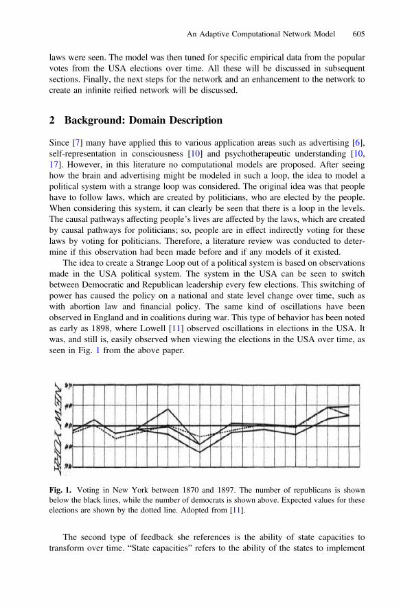
The Politicians Subnetwork. The next subnetwork devised concerns the causalpathways for the politicians and their parties. Figure 3 shows the politicians subnet-work. There is a limited resource of political power which is represented by an inputnode X21 for the politician level.

Fig. 2. Subnetwork for the individual level

608 J. Anten et al.

The people then vote for the political party they support, which then adjusts thecausal pathway for the resulting power each party has, which can be seen in the effectnodes X22 and X24. Within the causal pathways, the weights for each party (X35 andX36) are determined by the previous level. A negative connection between the twoparties, represents that the parties attempt to minimize the others influence.

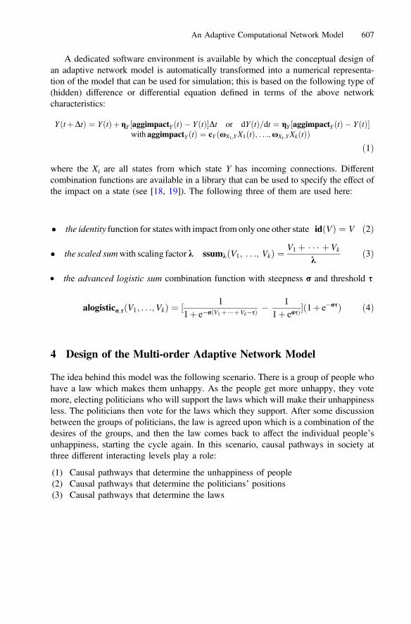
The Laws Subnetwork. The final subnetwork devised was for the law level; it can beseen in Fig. 4. In this network, there is a limited budget for laws, which is the inputnode X26. Given this budget, the political parties vote on either law 1 or law 2 (X27 orX28). Here the weights X22 and X24 (and also the scaling factors) are determined by theprevious level. After the vote, a logistic function is applied to the output of each of thelaws individually with a weight of 1, determining the new power of each law which isseen in the network as X52 and X53. Once the new power is determined, the effect ofeach law on the two groups is updated where the weights represent the effect of eachlaw on each of the groups. Finally for each of the two groups, the effect of the newcombination of laws is combined. These values for X33 and X34 become the new effectsof the laws on the two types of individuals.

Connections Between the Subnetworks. Now the subnetworks have been defined,the connections between them can be discussed. A simplified version of the networkcan be seen in Fig. 5, which shows how the networks are connected. Beginning withthe individual’s levels connections, the weight for the causal pathway from the input ofthe individual to the unhappiness of the individual is determined by the laws. Asdiscussed for the law subnetwork, nodes X33 and X34 represent how much an indi-vidual’s causal pathway of each group (rich or poor) is impacted by the current law

Fig. 3. Subnetwork for the politicians level

Fig. 4. Subnetwork for the law level

An Adaptive Computational Network Model 609

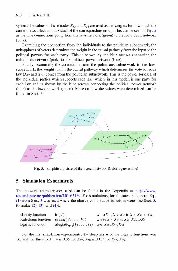
system; the values of these nodes X33 and X34 are used as the weights for how much thecurrent laws affect an individual of the corresponding group. This can be seen in Fig. 5as the blue connections going from the laws network (green) to the individuals network(pink).

Examining the connection from the individuals to the politician subnetwork, theunhappiness of voters determines the weight in the causal pathway from the input to thepolitical powers for each party. This is shown by the blue arrows connecting theindividuals network (pink) to the political power network (blue).

Finally, examining the connection from the politicians subnetwork to the lawssubnetwork, the weight within the causal pathway which determines the vote for eachlaw (X22 and X24) comes from the politician subnetwork. This is the power for each ofthe individual parties which supports each law, which, in this model, is one party foreach law and is shown by the blue arrows connecting the political power network(blue) to the laws network (green). More on how the values were determined can befound in Sect. 5.

5 Simulation Experiments

The network characteristics used can be found in the Appendix at https://www.researchgate.net/publication/340162169. For simulations, for all states the general Eq.(1) from Sect. 3 was used where the chosen combination functions were (see Sect. 3,formulae (2), (3), and (4)):

identity function idðVÞ X1 toX21;X26;X29 toX32;X39 toX48

scaled sum function ssumkðV1; . . .; VkÞ X22 toX25;X33 toX38;X49 toX51

logistic function alogisticr;sðV1; . . .;VkÞ X27;X28;X52;X53

For the first simulation experiments, the steepness r of the logistic functions was16, and the threshold s was 0.35 for X27, X28 and 0.7 for X52, X53.

Fig. 5. Simplified picture of the overall network (Color figure online)

610 J. Anten et al.

From the literature, it was seen that the system should oscillate, therefore in the firstrun of the model this behaviour was searched for. For the first simulation both groupswere initialized with the same values (or worth). This meant the groups have the sameunhappiness if their preferred law is not active. For some parameter settings thebehaviour was observed as seen in Fig. 6. The unhappiness of the people can be seen tooscillate between the two groups, as well as the laws the political power. This figureactually shows the unhappiness of one representative person for each group, not thetotal unhappiness of the group. All persons in the group show the exact same behavior,since they are initialized the same and influenced by the same law. It can be seen that arise in political power for a group closely follows the rise of unhappiness in that samegroup and that the laws preferred by a group follow slower, but they do rise when thepolitical power of that group rises. This can be explained by the slower speed factorsassociated to the laws. All the oscillations now have the same amplitude, since allgroups and laws are initialized either exactly the same or in the case of the laws at 1 forthe poor law and 0 for the rich law.

To get the model to simulate real societies better, in the following simulation thetwo groups were initialized differently. The “rich” group was initialized with a score (orincome) of 0.8 and the “poor” group with a score (or income) of 0.4. This meant thatthe rich people will have the ability to have a much higher unhappiness than the poorpeople, so it is expected the “rich” group will have a higher political power and gettheir preferred law more active than the law preferred by the “poor” people. Thebehavior resulting from this simulation can be seen in Fig. 7.

The “rich” law is always more active than the “poor” law, and although there arestill some oscillations, the “poor” group only gets influence when they are veryunhappy and are always less influential than the “rich” group, which is to be expectedwhen there is a group which is more influential than the other with the same number ofpeople.

Fig. 6. Behavior for the first run with oscillations

An Adaptive Computational Network Model 611

6 Further Validation of the Network Model

Data from the popular votes of the United States presidential elections was collectedfrom the USA archive (archives.gov), and plotted using the percentage of republicanand democratic votes. This data was then used to validate the model. A graph of thisdata can be seen in Fig. 8. Oscillations between the two parties are clearly visible here.Both the initial simulation and the analysis of popular votes, shows the same trend,where oscillations between the two “parties” can be seen. The difference is in the sizeof the oscillations. The popular votes simulation has small oscillations between 0.65and 0.35, while the initial model has oscillations between 0.8 and 0.2.

Parallels can be drawn between the behavior of the model with the groups ini-tialized differently. Continuing to follow the rich and poor example, in real life thereare less rich people, but they are still very influential. Looking at Fig. 7, it can be seenthat the rich easily overpower the poor.

The model was tuned on these data from US elections. Speed factors were tuned forX21 until X48, and for X52 and X53. Furthermore, the sigma’s and tau’s for the alogisticfunctions of X27, X28, X52 and X53 were also tuned. These are the nodes for voting for

Fig. 7. Behaviour for different initial values of the rich and poor groups

Fig. 8. Statistics for the US presidential elections

612 J. Anten et al.

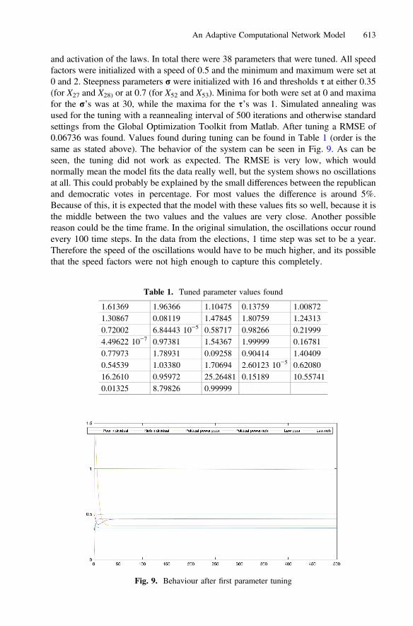
and activation of the laws. In total there were 38 parameters that were tuned. All speedfactors were initialized with a speed of 0.5 and the minimum and maximum were set at0 and 2. Steepness parameters r were initialized with 16 and thresholds s at either 0.35(for X27 and X28) or at 0.7 (for X52 and X53). Minima for both were set at 0 and maximafor the r’s was at 30, while the maxima for the s’s was 1. Simulated annealing wasused for the tuning with a reannealing interval of 500 iterations and otherwise standardsettings from the Global Optimization Toolkit from Matlab. After tuning a RMSE of0.06736 was found. Values found during tuning can be found in Table 1 (order is thesame as stated above). The behavior of the system can be seen in Fig. 9. As can beseen, the tuning did not work as expected. The RMSE is very low, which wouldnormally mean the model fits the data really well, but the system shows no oscillationsat all. This could probably be explained by the small differences between the republicanand democratic votes in percentage. For most values the difference is around 5%.Because of this, it is expected that the model with these values fits so well, because it isthe middle between the two values and the values are very close. Another possiblereason could be the time frame. In the original simulation, the oscillations occur roundevery 100 time steps. In the data from the elections, 1 time step was set to be a year.Therefore the speed of the oscillations would have to be much higher, and its possiblethat the speed factors were not high enough to capture this completely.

Table 1. Tuned parameter values found

1.61369 1.96366 1.10475 0.13759 1.008721.30867 0.08119 1.47845 1.80759 1.243130.72002 6.84443 10−5 0.58717 0.98266 0.219994.49622 10−7 0.97381 1.54367 1.99999 0.167810.77973 1.78931 0.09258 0.90414 1.404090.54539 1.03380 1.70694 2.60123 10−5 0.6208016.2610 0.95972 25.26481 0.15189 10.557410.01325 8.79826 0.99999

Fig. 9. Behaviour after first parameter tuning

An Adaptive Computational Network Model 613

To overcome this, we exaggerated the empirical data and put it at 0.5, 1 and 0 inalternating order with 48 time steps between, which is 4 years in terms of months.Figure 10 shows the empirical data and the simulation data for this and as can be seen,oscillations did occur with the exaggerated data. RMSE behavior can be seen in Fig. 10and shows that the lowest RMSE value was found at the beginning and after that neveragain. This could occur due to a couple of reasons. Either, this minimum score isdifficult to reach and after leaving the optimum, it is unlikely to find back again due tothe specificity of the values. It could be to do with the reannealing interval after 100iterations, which makes the temperature rise again, so less optimal solutions are againaccepted without giving time to search the space for more optimum values. Evidencefor this could be seen in Fig. 10, since sometimes it seems to trend down as expectedfrom simulated annealing and after which the RMSE rises again.

Fig. 10. Upper graph: behaviour after second parameter tuning. Lower graph: RMSE overiterations

614 J. Anten et al.

It could also be due to trying to fit the wrong parameters, since less parameters werefitted for this tuning. Only the r’s and the s’s of the activation of the laws and theirspeed factors were tuned as it was thought that these would be the parameters thatwould affect the general shape the most.

7 Discussion and Future Work

In the first simulation run, in a qualitative sense the network behaved as expected fromthe research done, with the political powers oscillating between rich party being inpower and the poor party being in power in periodic oscillations. In the initial simu-lation, seen in Fig. 6, it can be seen that as the poor parties unhappiness is rising, thepolitical power of the poor group rises as well, then about 90 degrees out of phase, thepoor law begins to increase. As the law increases, the unhappiness begins to decreaseand the rich groups unhappiness increases as they are dissatisfied with the situation andbegin to vote more. This same behaviour is also seen in the rich group, about 180degrees out of phase. The laws oscillate around 0.5 for both the poor and the rich.

When initializing the individuals groups (rich and poor) with different startingvalues as seen in Fig. 7, the periodic oscillation behaviour is still seen, but the center ofthese oscillations for each group is different. The value at which the laws oscillatearound is approximately 0.8 for the rich and 0.33 for the poor compared to those seenin the previous simulation at 0.5 each. This behaviour is expected as the rich group hasmore unhappiness since they have more wealth to lose. This means that they will bemore active in ensuring that their law, which benefits them more, is in effect, where thepoor people’s unhappiness is relatively small compared to them so they don’t have theability to compete. This can be seen in real life politics, as the rich have more ability toinfluence politics due to the influence and money they have, where the poor often haveto struggle and campaign much harder to get change.

When tuning the model to the numerical data from the USA, it was seen that themodel showed no oscillations. One reason this could occur is that since the data doesnot oscillate much outside of 0.5, the mean is the best optimum that system can reachfrom those starting values. Another reason could be due to the levels of the parametersbeing tuned not being high enough, or the assumed number of steps for the modelbeing too small, as one time step was set to a year. When observing the originalnetwork simulation, it can be seen that an oscillation occurred once approximatelyevery 100 steps. Therefor, if the data was set to months rather than years (48 stepsbetween oscillations rather than 4) or if the speed factors were allowed to increaseabove 2, the network may have converged to periodic oscillation.

In the future it would be interesting to see how increasing the number of poorpeople would affect the system. From observing politics in real life situations, if thereare enough poor people, the activation of the rich law should decrease, as there is morereactive unhappiness coming from the poor group. This was not done in this experi-ment as there was not enough time to update and modify the network.

Another interesting addition to a future version of the model would be to add inmultiple laws. This would require more complex individuals, with nodes for each of thedifferent issues and then a general unhappiness. The political level would also have to

An Adaptive Computational Network Model 615

be updated to reflect the multiple laws each party could vote for. This would also openthe model to have parties who voted for the laws in different ways and having theindividuals vote for the parties who best reflected where the largest unhappiness wascoming from.

Towards the end of the experiment, a network with add in media to the system wasdevised. In this network the upwards connections would be from the people to themedia, where the people affect what the media talks about based off their interests andviews. Then the media would affect the politicians by enhancing or detracting fromhow the people view them. The people would have an upward connection to politiciansto vote for them as before. The politicians would then effect the laws in the same waythey do now through voting and finally the laws would affect the people in a similarway.

The downward connections, starting with the laws, would be the laws affect thepoliticians through changing how the voting works and/or the speed factors. Thepoliticians would affect the media through what equates to forcing them to talk posi-tively or negatively about certain topics or suppression of others. The media wouldenhance or dampen the peoples reactions/care for the policies and laws. Finally thepeople would affect the laws by determining how quickly the laws come into effect dueto how well they are followed/received by the population.

In future developments, a number of other relevant subtleties can be addressed aswell. For example, for the US, the important roles of the hierarchy from cities to statesto federal level, of competing lobby groups, and of the differences in access toinformation for different subpopulations can be addressed.

8 Conclusion

In the reported research an experiment of a strange loop adaptive temporal-causalnetwork was created, tested and validated to reflect political oscillations as seen inpresidential elections. The temporal network breaks a political system into 3 groups,the individual people, the politicians, and the laws where the individuals feed into thepoliticians, who feed into the laws, which feed into the individuals. In the initialsimulation, the oscillatory behaviour which was expected from the literature reviewwas observed. Next the network was modified to reflect an unbalanced political systemwith one group of individuals that were influenced more by the laws than the other.This cause the law which benefited those with more influence to be higher than the lawwhich was beneficial for those with less influence, as expected. Finally the network wastuned to data from the USA presidential elections popular vote using simulatedannealing, with both actual and simplified data. The simulated annealing did not per-form as expected, giving a network which did not oscillate when using the real data,when using the simplified data, managed to reflect the behaviour which it was tuned on.The network not being able to tune on the real data could be due to the oscillations databeing so close to 0.5, that the model found 0.5 as the ideal with the initial setting givenand was unable to escape to another optimum. Another possible reason would be thatthe speed factors not being allowed to be tuned above 2 or due to the small number ofsteps between oscillations.

616 J. Anten et al.

References

1. Baumgartner, F.R., Jones, B.D.: Policy Dynamics. University of Chicago Press (2002)2. Davis, R.: Meta-rules: reasoning about control. Artif. Intell. 15, 179–222 (1980)3. Davis, R., Buchanan, B.G.: Meta-level knowledge: overview and applications. In:

Proceedings of 5th IJCAI, pp. 920–927 (1977)4. Galton, A.: Operators vs. arguments: the ins and outs of reification. Synthese 150, 415–441

(2006)5. Hebb, D.O.: The Organization of Behavior: A Neuropsychological Theory. Wiley, London

(1949)6. Hendlin, Y.H.: I am a fake loop: the effects of advertising-based artificial selection.

Biosemiotics 12(1), 131–156 (2019)7. Hofstadter, D.R.: Gödel, Escher, Bach. Basic Books, New York (1979)8. Hofstadter, D.R.: What is it like to be a strange loop? In: Kriegel, U., Williford, K. (eds.)

Self-Representational Approaches to Consciousness. MIT Press, Cambridge (2006)9. Hofstadter, D.R.: I Am a Strange Loop. Basic Books, New York (2007)10. Kriegel, U., Williford, K.: Self-representational Approaches to Consciousness. MIT Press,

Cambridge (2006)11. Lowell, A.L.: Oscillations in politics. Ann. Am. Acad. Polit. Soc. Sci. 12, 69–97 (1898).

https://doi.org/10.1177/00027162980120010412. Nagel, E., Newman, J.: Gödel’s Proof. New York University Press, New York (1965)13. Pierson, P.: When effect becomes cause: policy feedback and political change. World Polit.

45, 595–628 (1993). https://doi.org/10.2307/295071014. Skocpol, T.: Protecting Soldiers and Mothers: The Political Origins of Social Policy in the

United States. Belknap Press of Harvard, Cambridge (2009). https://doi.org/10.2307/j.ctvjz81v6

15. Smorynski, C.: The incompleteness theorems. In: Barwise, J. (ed.) Handbook ofMathematical Logic, vol. 4, pp. 821–865. North-Holland, Amsterdam (1977)

16. Sterling, L., Beer, R.: Metainterpreters for expert system construction. J. Logic Program. 6,163–178 (1989)

17. Strijbos, D., Glas, G.: Self-knowledge in personality disorder: self-referentiality as a steppingstone for psychotherapeutic understanding. J. Pers. Disorders 32(3), 295–310 (2018)

18. Treur, J.: Network-Oriented Modeling: Addressing Complexity of Cognitive, Affective andSocial Interactions. Springer, Heidelberg (2016). https://doi.org/10.1007/978-3-319-45213-5

19. Treur, J.: Network-Oriented Modeling for Adaptive Networks: Designing Higher-OrderAdaptive Biological, Mental and Social Network Models. Springer, Heidelberg (2020).https://doi.org/10.1007/978-3-030-31445-3

20. Weyhrauch, R.W.: Prolegomena to a theory of mechanized formal reasoning. Artif. Intell.13, 133–170 (1980)

An Adaptive Computational Network Model 617