Amplitude Variation with

Offset

presented byRoxy Frary

TheoryJust some background

…ok a lot of background

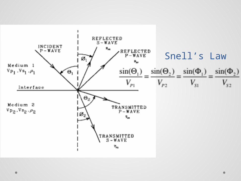
Snell’s Law

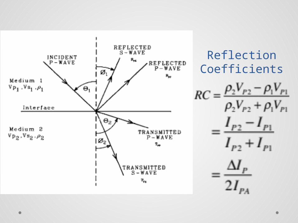
Reflection Coefficients

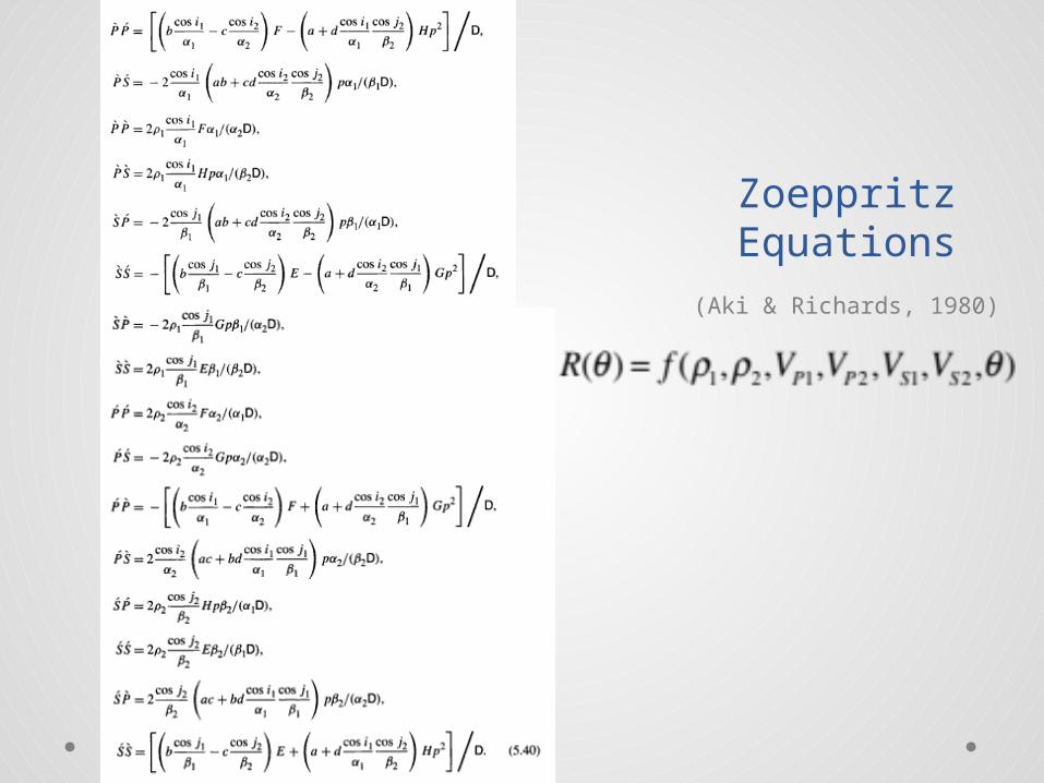
Zoeppritz Equations

(Aki & Richards, 1980)

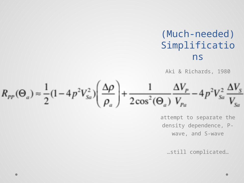
(Much-needed) Simplifications

Aki & Richards, 1980

attempt to separate the

density dependence, P-

wave, and S-wave

…still complicated…

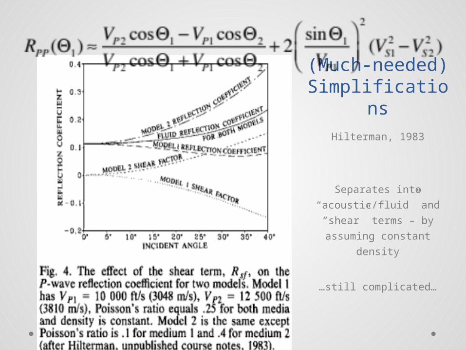
(Much-needed) Simplifications

Hilterman, 1983

Separates into

“acoustic/fluid” and

“shear” terms – by

assuming constant density

…still complicated…

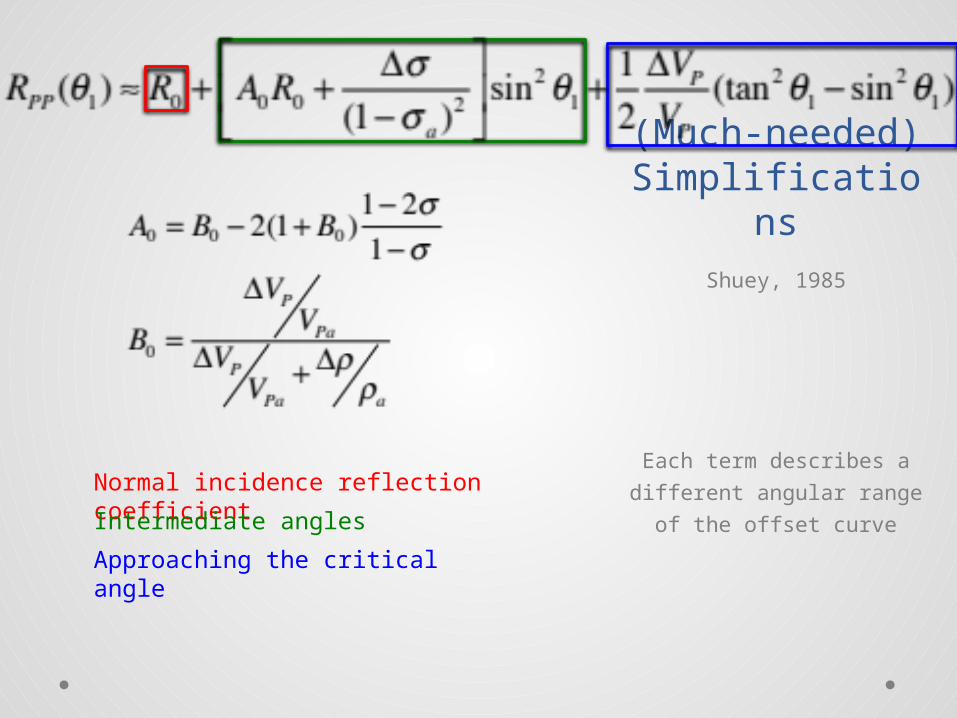
(Much-needed) Simplifications

Shuey, 1985

Each term describes a

different angular range of

the offset curve

Normal incidence reflection coefficientIntermediate angles

Approaching the critical angle

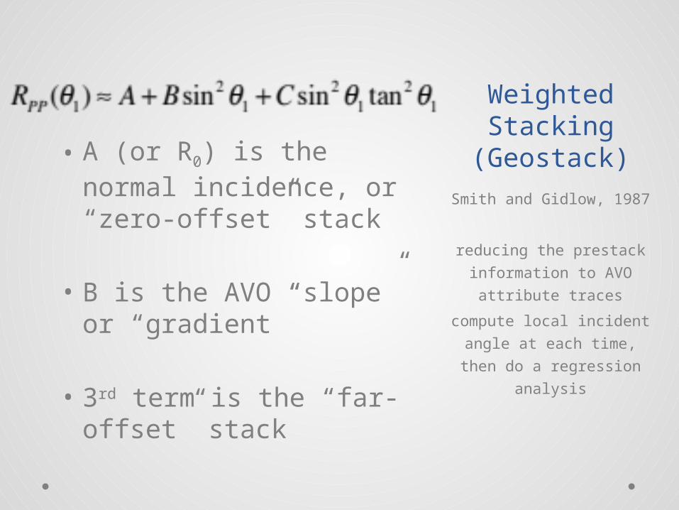
Weighted Stacking

(Geostack)Smith and Gidlow, 1987

reducing the prestack

information to AVO

attribute traces

compute local incident

angle at each time, then do

a regression analysis

• A (or R0) is the normal incidence, or “zero-offset” stack

• B is the AVO “slope” or “gradient”

• 3rd term is the “far-offset” stack

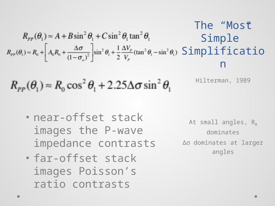
The “Most Simple”

SimplificationHilterman, 1989

At small angles, R0

dominates

Δσ dominates at larger

angles

• near-offset stack images the P-wave impedance contrasts

• far-offset stack images Poisson’s ratio contrasts

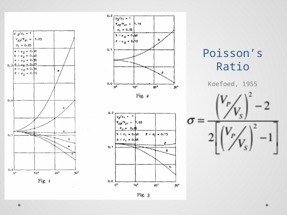
Poisson’s RatioKoefoed, 1955

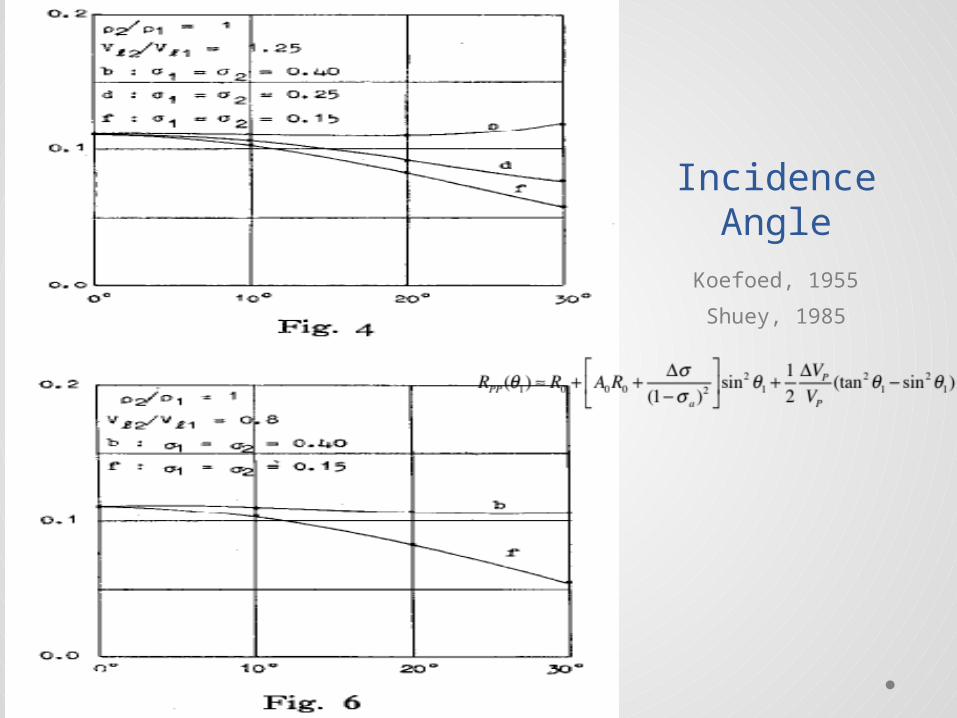
Incidence Angle

Koefoed, 1955

Shuey, 1985

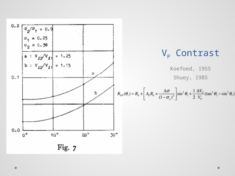
VP Contrast

Koefoed, 1955

Shuey, 1985

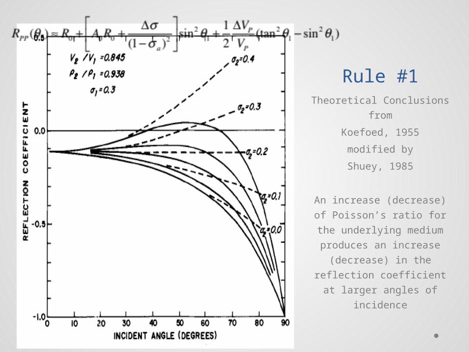
Rule #1Theoretical Conclusions

from

Koefoed, 1955

modified by

Shuey, 1985

An increase (decrease) of

Poisson’s ratio for the

underlying medium

produces an increase

(decrease) in the reflection

coefficient at larger angles

of incidence

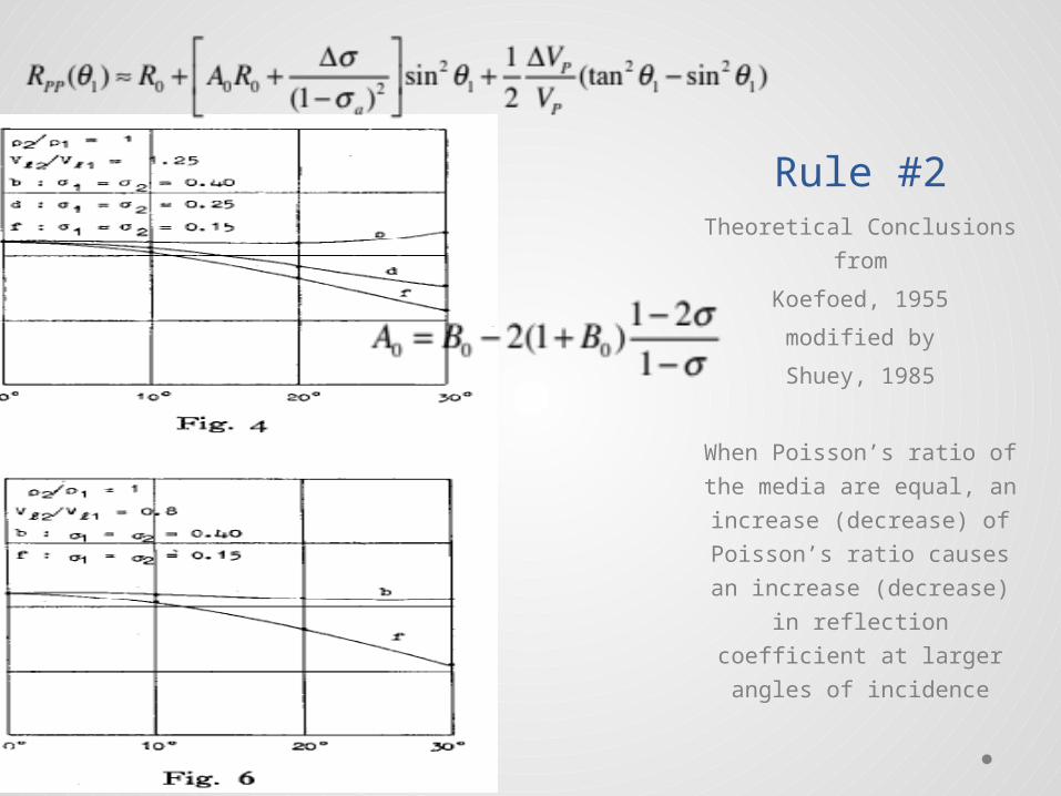
Rule #2Theoretical Conclusions

from

Koefoed, 1955

modified by

Shuey, 1985

When Poisson’s ratio of the

media are equal, an

increase (decrease) of

Poisson’s ratio causes an

increase (decrease) in

reflection coefficient at

larger angles of incidence

Rule #3Theoretical Conclusions

from

Koefoed, 1955

modified by

Shuey, 1985

Interchange of the media

affects the shape of the

curves only slightly – RPP

simply changes sign when

the elastic properties are

interchanged – except at

large angles

Industry Use:Gas Sands

Since 1982

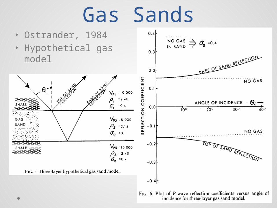
Gas Sands• Ostrander, 1984• Hypothetical gas

model

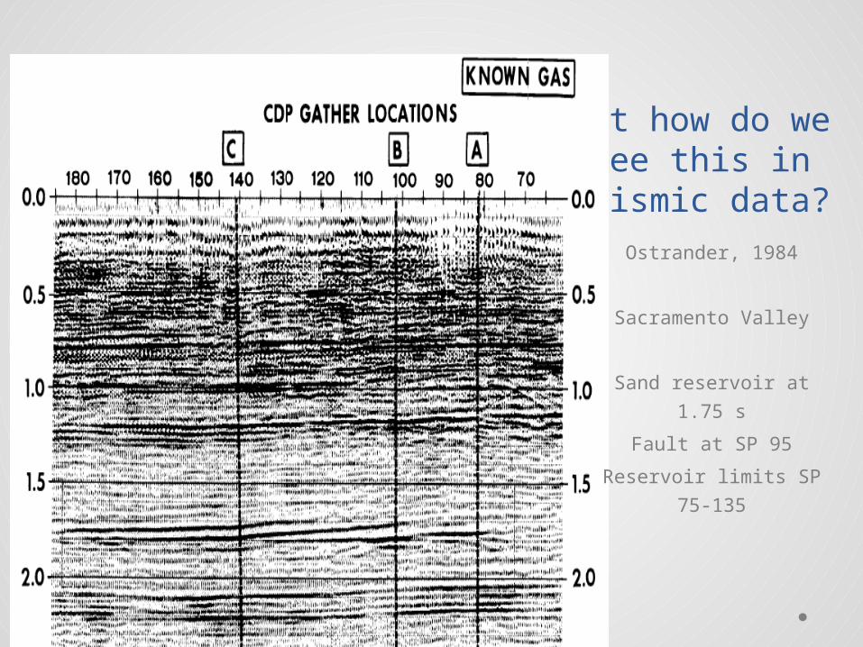
But how do we see this in

seismic data?Ostrander, 1984

Sacramento Valley

Sand reservoir at 1.75 s

Fault at SP 95

Reservoir limits SP 75-

135

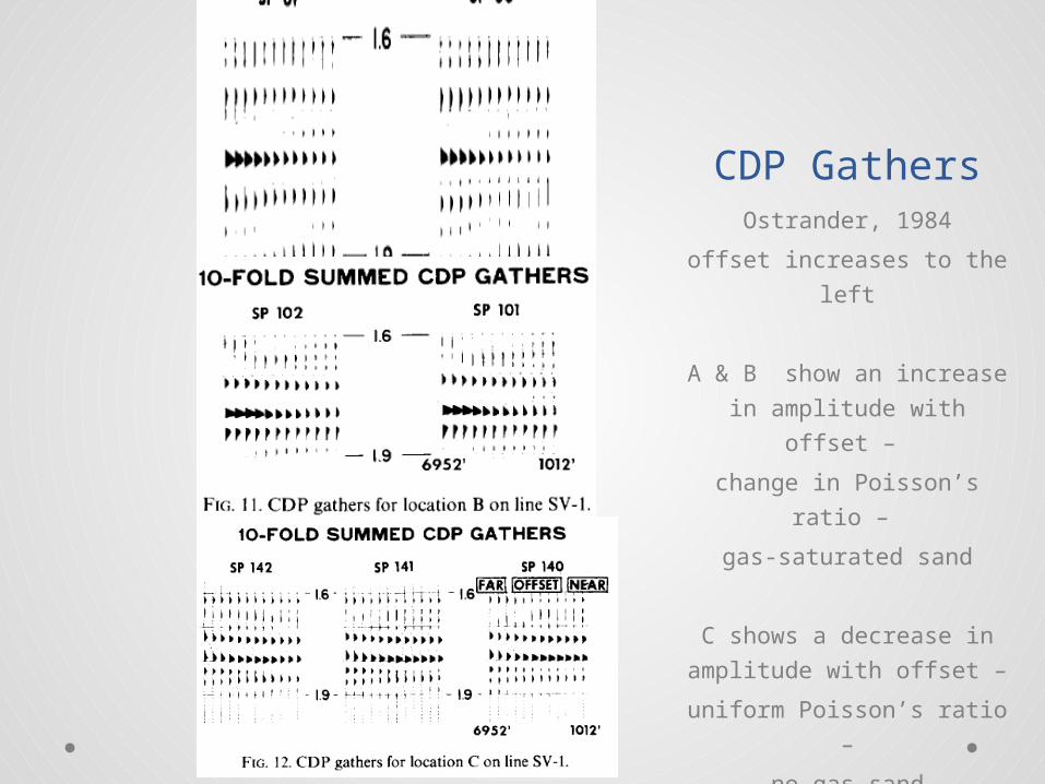
CDP GathersOstrander, 1984

offset increases to the left

A & B show an increase in

amplitude with offset –

change in Poisson’s ratio –

gas-saturated sand

C shows a decrease in

amplitude with offset –

uniform Poisson’s ratio –

no gas sand

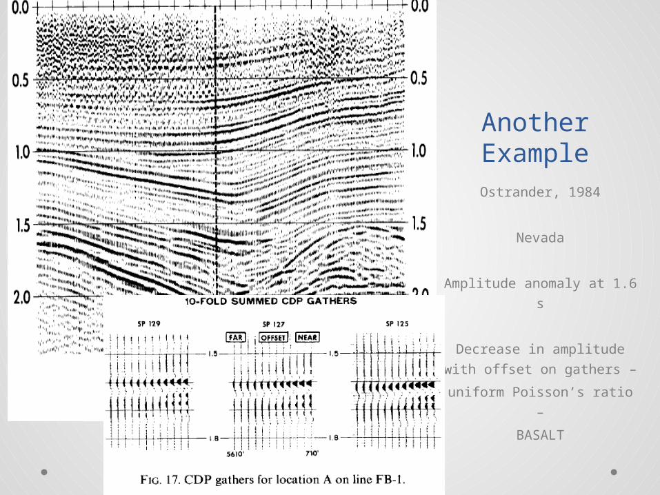
Another ExampleOstrander, 1984

Nevada

Amplitude anomaly at 1.6

s

Decrease in amplitude

with offset on gathers –

uniform Poisson’s ratio –

BASALT

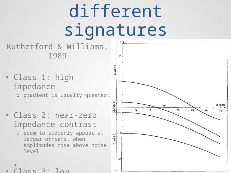
But different Gas Sands have different

signaturesRutherford & Williams,

1989

• Class 1: high impedanceo gradient is usually greatest

• Class 2: near-zero impedance contrasto seem to suddenly appear at

larger offsets, when amplitudes rise above noise level

• Class 3: low impedanceo large reflectivities at all offsets

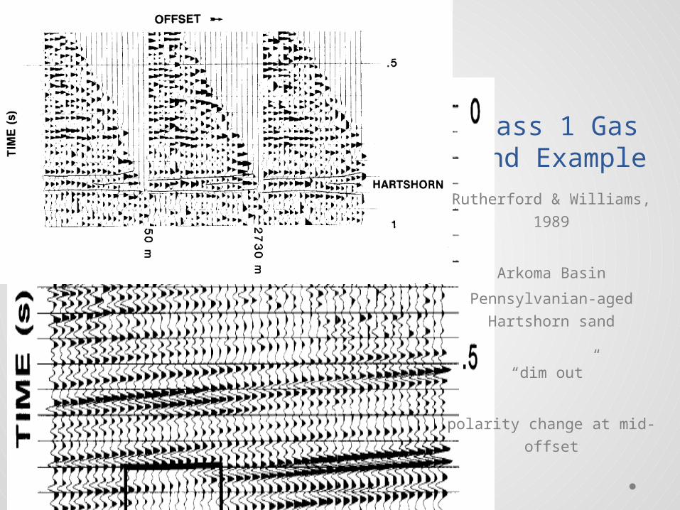
Class 1 Gas Sand Example

Rutherford & Williams,

1989

Arkoma Basin

Pennsylvanian-aged

Hartshorn sand

“dim out”

polarity change at mid-

offset

Class 2 Gas Sand Example

Rutherford & Williams,

1989

Gulf of Mexico

Brazos area

mid-Miocene

not a classic “gas sand”

anomaly – 2.1 s

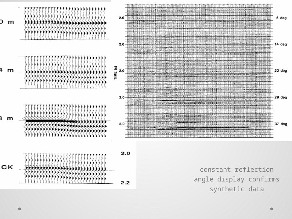
Class 2 Gas Sand Example

(Cont’d)Rutherford & Williams,

1989

AVO effects are

pronounced in mid- and far-

offset synthetics

constant reflection angle

display confirms synthetic

data

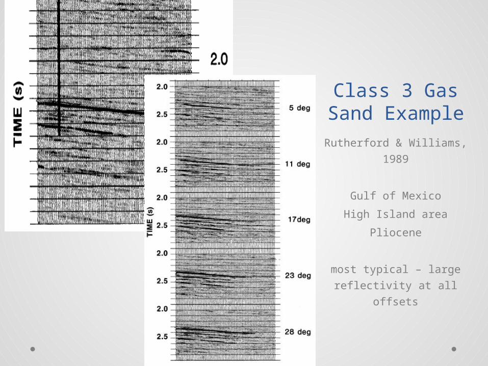
Class 3 Gas Sand Example

Rutherford & Williams,

1989

Gulf of Mexico

High Island area

Pliocene

most typical – large

reflectivity at all offsets

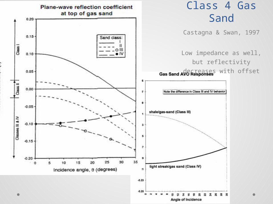
Class 4 Gas Sand

Castagna & Swan, 1997

Low impedance as well, but

reflectivity decreases with

offset

Industry Use:Fluid Identification

Since 1997

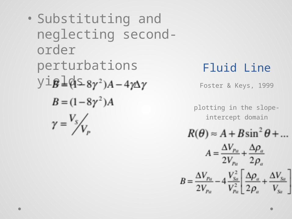
Fluid Line

• Substituting and neglecting second-order perturbations yields

Foster & Keys, 1999

plotting in the slope-

intercept domain

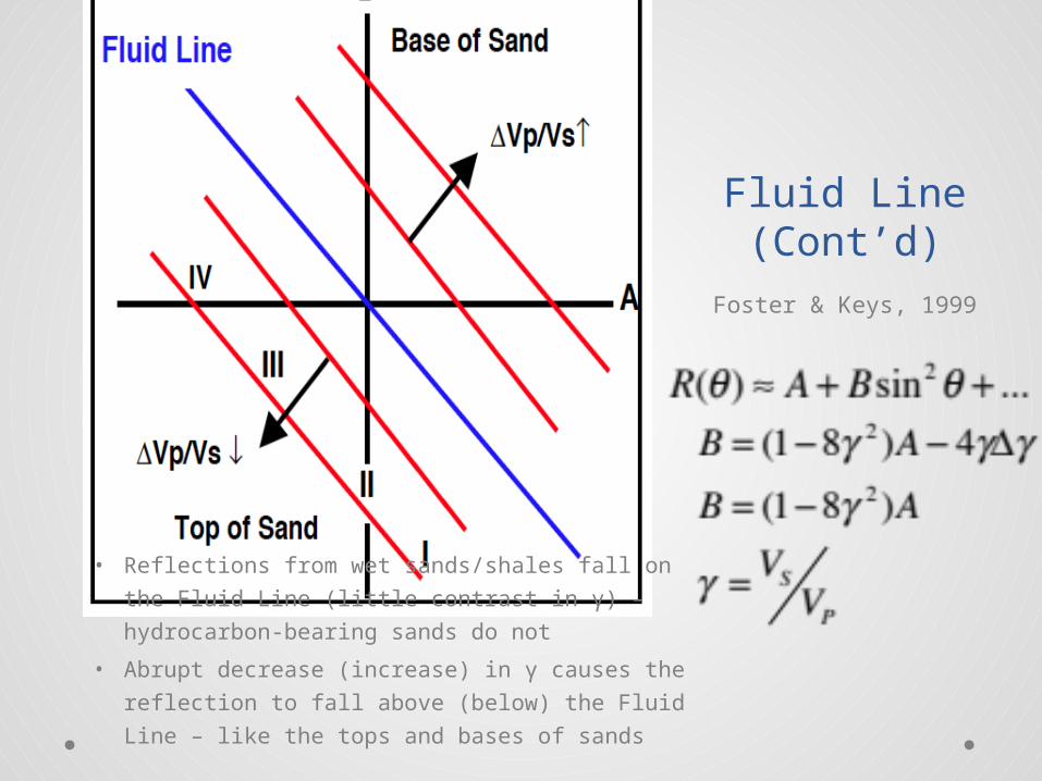
Fluid Line (Cont’d)

Foster & Keys, 1999

• Reflections from wet sands/shales fall on the

Fluid Line (little contrast in γ) – hydrocarbon-

bearing sands do not

• Abrupt decrease (increase) in γ causes the

reflection to fall above (below) the Fluid Line –

like the tops and bases of sands

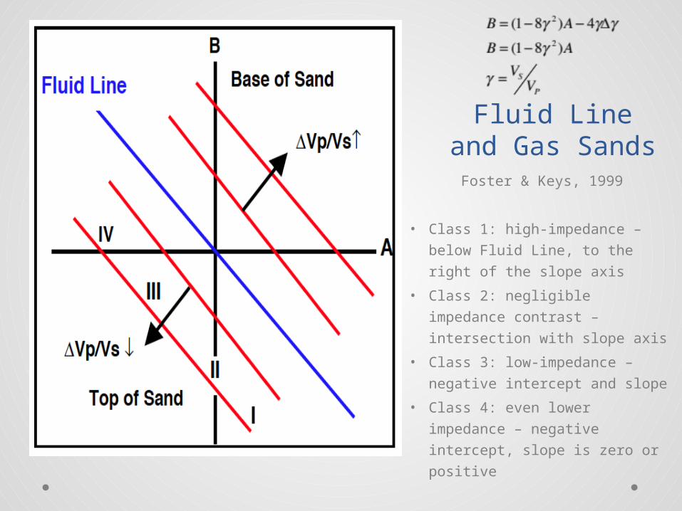
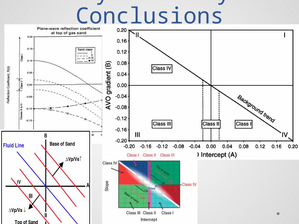
Fluid Line and Gas Sands

Foster & Keys, 1999

• Class 1: high-impedance –

below Fluid Line, to the right of

the slope axis

• Class 2: negligible impedance

contrast – intersection with

slope axis

• Class 3: low-impedance –

negative intercept and slope

• Class 4: even lower impedance

– negative intercept, slope is

zero or positive

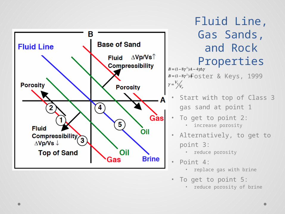
Fluid Line, Gas Sands, and

Rock Properties

Foster & Keys, 1999

• Start with top of Class 3 gas

sand at point 1

• To get to point 2:• increase porosity

• Alternatively, to get to point 3:• reduce porosity

• Point 4:• replace gas with brine

• To get to point 5:• reduce porosity of brine

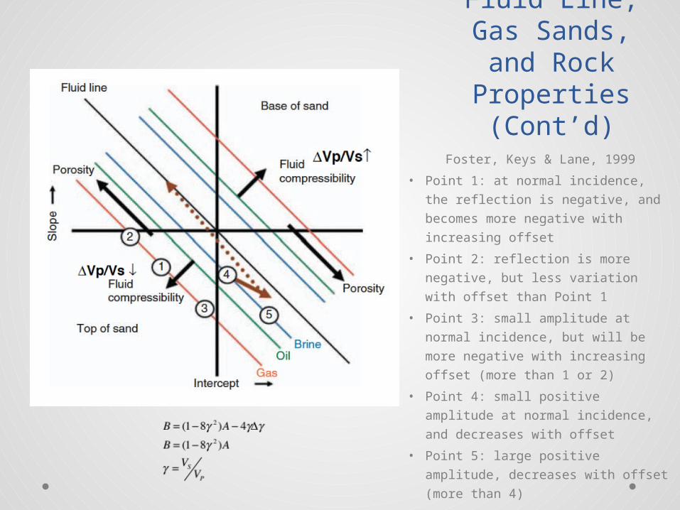
Fluid Line, Gas Sands, and

Rock Properties (Cont’d)

Foster, Keys & Lane, 1999

• Point 1: at normal incidence, the

reflection is negative, and becomes

more negative with increasing offset

• Point 2: reflection is more negative,

but less variation with offset than

Point 1

• Point 3: small amplitude at normal

incidence, but will be more negative

with increasing offset (more than 1

or 2)

• Point 4: small positive amplitude at

normal incidence, and decreases

with offset

• Point 5: large positive amplitude,

decreases with offset (more than 4)

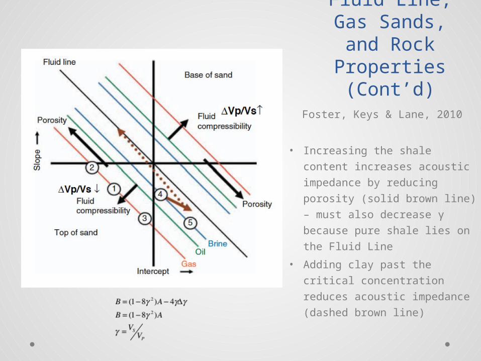
Fluid Line, Gas Sands, and

Rock Properties (Cont’d)

Foster, Keys & Lane, 2010

• Increasing the shale content

increases acoustic impedance

by reducing porosity (solid

brown line) – must also

decrease γ because pure shale

lies on the Fluid Line

• Adding clay past the critical

concentration reduces acoustic

impedance (dashed brown line)

AVO for hydrocarbon detection

Foster, Keys & Lane, 2010

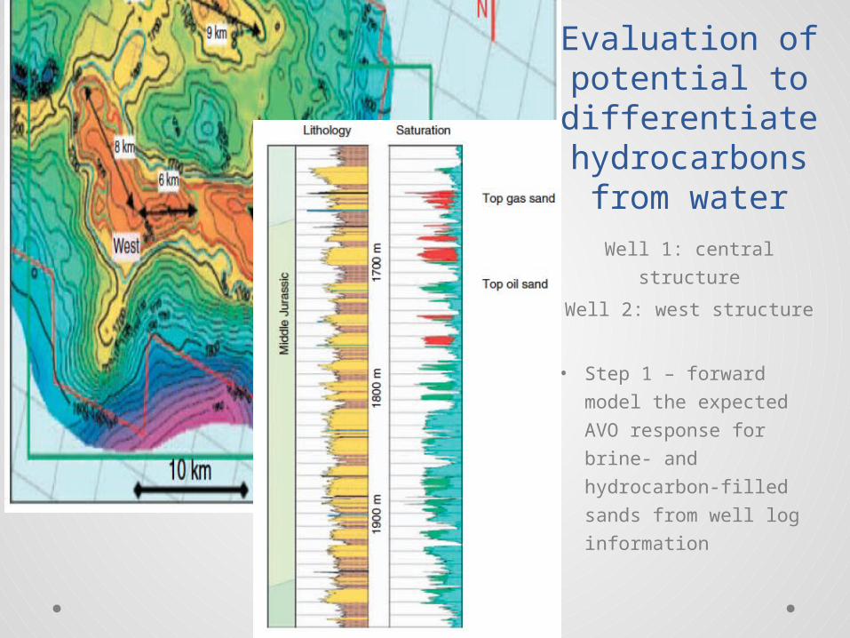
Evaluation of potential to differentiate

hydrocarbons from water

Well 1: central structure

Well 2: west structure

• Step 1 – forward model

the expected AVO

response for brine- and

hydrocarbon-filled sands

from well log

information

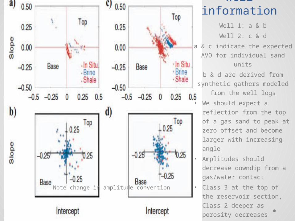
Well information

Well 1: a & b

Well 2: c & d

a & c indicate the expected

AVO for individual sand units

b & d are derived from

synthetic gathers modeled

from the well logs

• We should expect a

reflection from the top of a

gas sand to peak at zero

offset and become larger

with increasing angle

• Amplitudes should

decrease downdip from a

gas/water contact

• Class 3 at the top of the

reservoir section, Class 2

deeper as porosity

decreases

Note change in amplitude convention

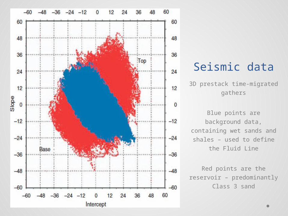
Seismic data3D prestack time-migrated

gathers

Blue points are background

data, containing wet sands

and shales – used to define

the Fluid Line

Red points are the reservoir

– predominantly Class 3

sand

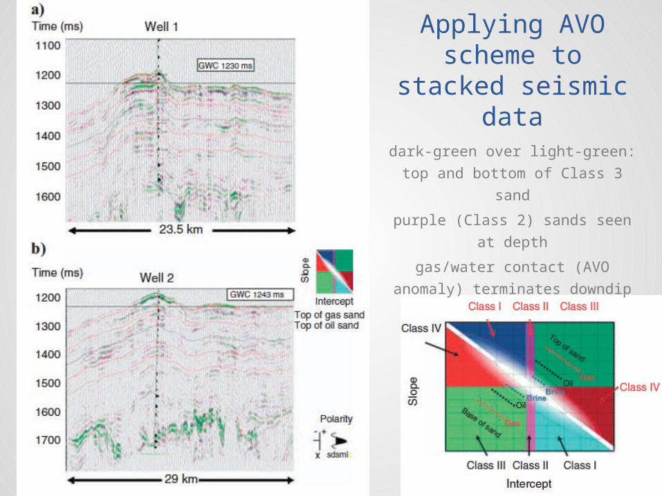
Applying AVO scheme to stacked

seismic datadark-green over light-green: top

and bottom of Class 3 sand

purple (Class 2) sands seen at

depth

gas/water contact (AVO anomaly)

terminates downdip

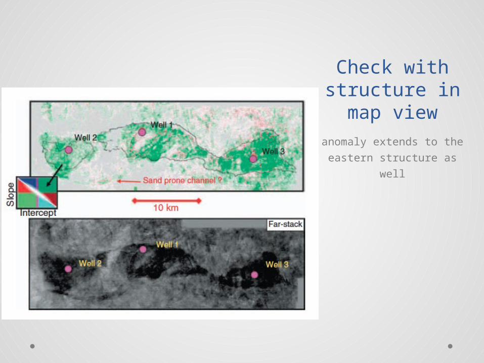
Check with structure in map view

anomaly extends to the

eastern structure as well

AVO for lithology discrimination

Foster, Keys & Lane, 2010

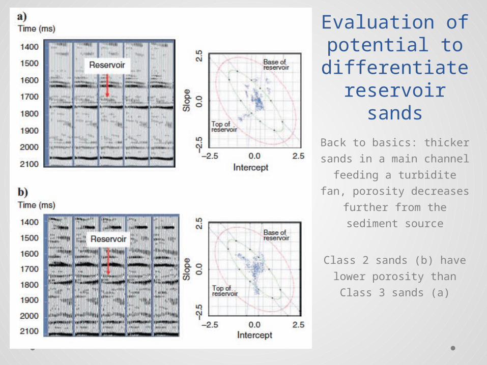
Evaluation of potential to differentiate

reservoir sandsBack to basics: thicker

sands in a main channel

feeding a turbidite fan,

porosity decreases further

from the sediment source

Class 2 sands (b) have

lower porosity than Class 3

sands (a)

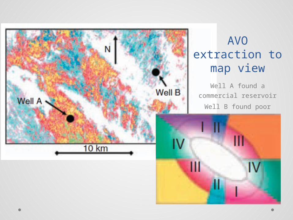
AVO extraction to map view

Well A found a commercial

reservoir

Well B found poor porosity

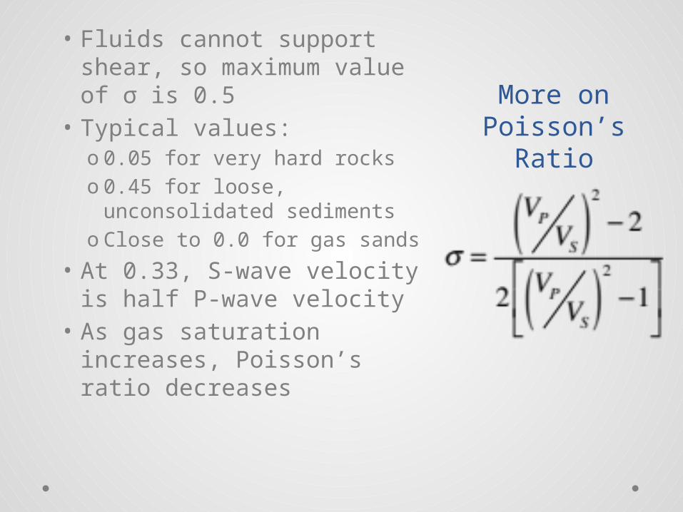
More on Poisson’s Ratio

• Fluids cannot support shear, so maximum value of σ is 0.5

• Typical values:o 0.05 for very hard rockso 0.45 for loose,

unconsolidated sedimentso Close to 0.0 for gas sands

• At 0.33, S-wave velocity is half P-wave velocity

• As gas saturation increases, Poisson’s ratio decreases

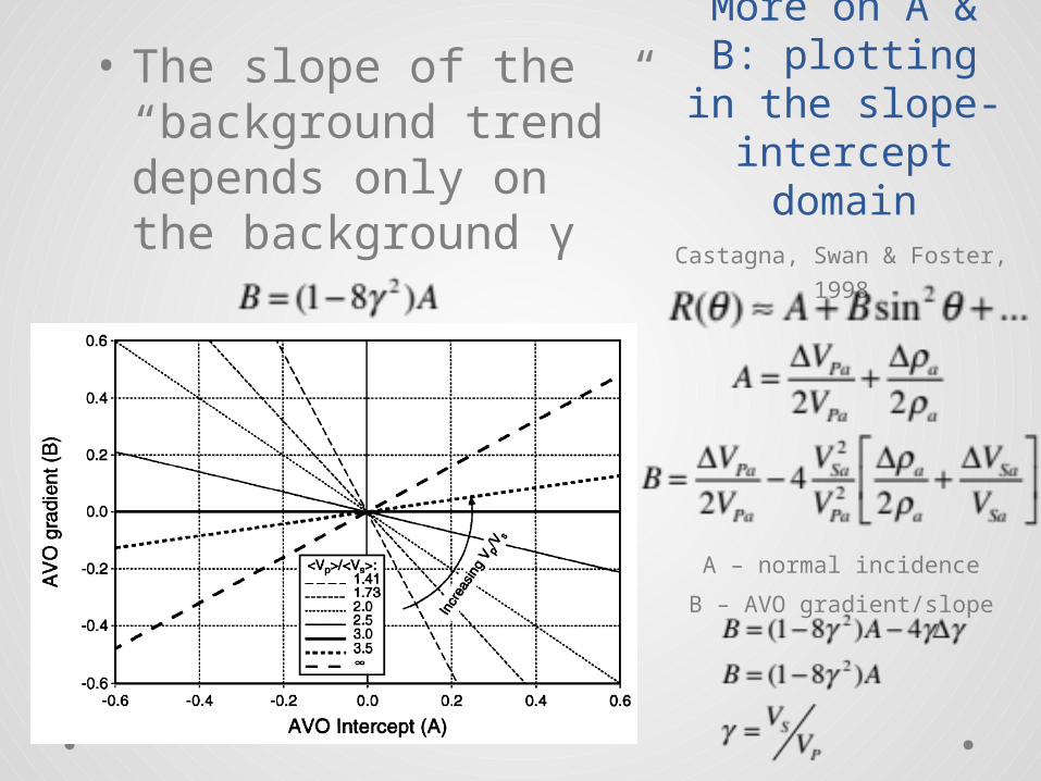
More on A & B: plotting in the slope-intercept

domain

• The slope of the “background trend” depends only on the background γ

Castagna, Swan & Foster,

1998

A – normal incidence

B – AVO gradient/slope

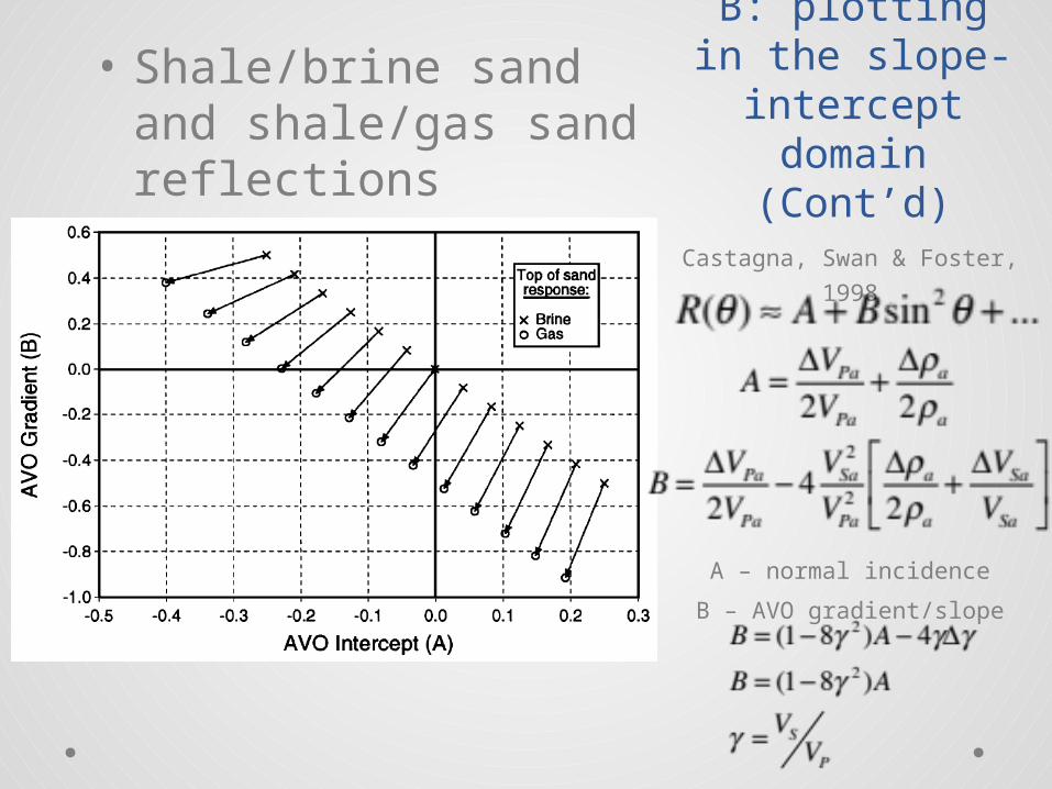
More on A & B: plotting in the slope-intercept

domain (Cont’d)

• Shale/brine sand and shale/gas sand reflections

Castagna, Swan & Foster,

1998

A – normal incidence

B – AVO gradient/slope

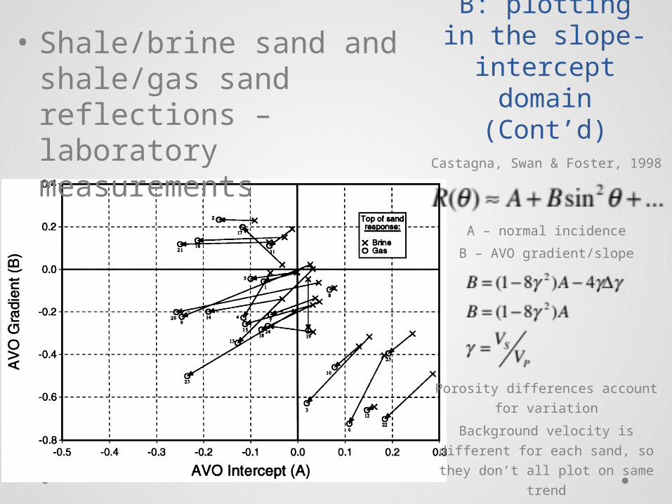
More on A & B: plotting in the slope-intercept

domain (Cont’d)

• Shale/brine sand and shale/gas sand reflections – laboratory measurements

Castagna, Swan & Foster, 1998

A – normal incidence

B – AVO gradient/slope

Porosity differences account for

variation

Background velocity is different

for each sand, so they don’t all

plot on same trend

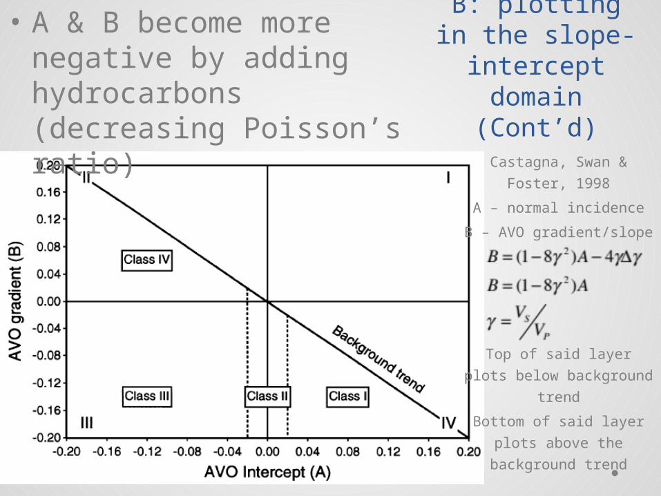
More on A & B: plotting in the slope-intercept

domain (Cont’d)

• A & B become more negative by adding hydrocarbons (decreasing Poisson’s ratio)

Castagna, Swan & Foster,

1998

A – normal incidence

B – AVO gradient/slope

Top of said layer plots

below background trend

Bottom of said layer plots

above the background

trend

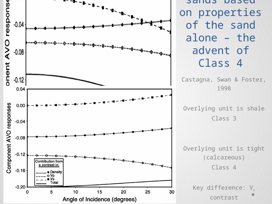
Can’t classify sands based on properties of

the sand alone – the advent of

Class 4Castagna, Swan & Foster,

1998

Overlying unit is shale

Class 3

Overlying unit is tight

(calcareous)

Class 4

Key difference: Vs contrast

Case HistoryGulf of Mexico Bright Spot

Nsoga Mahob, Castagna & Young, 1999

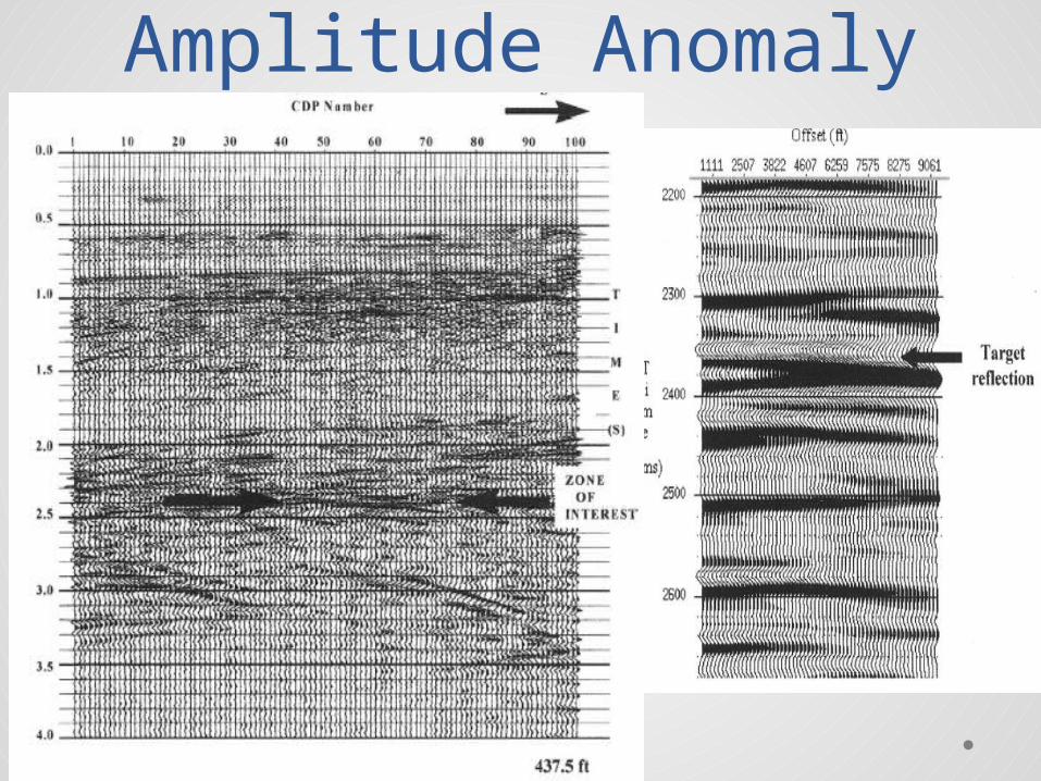
Amplitude Anomaly

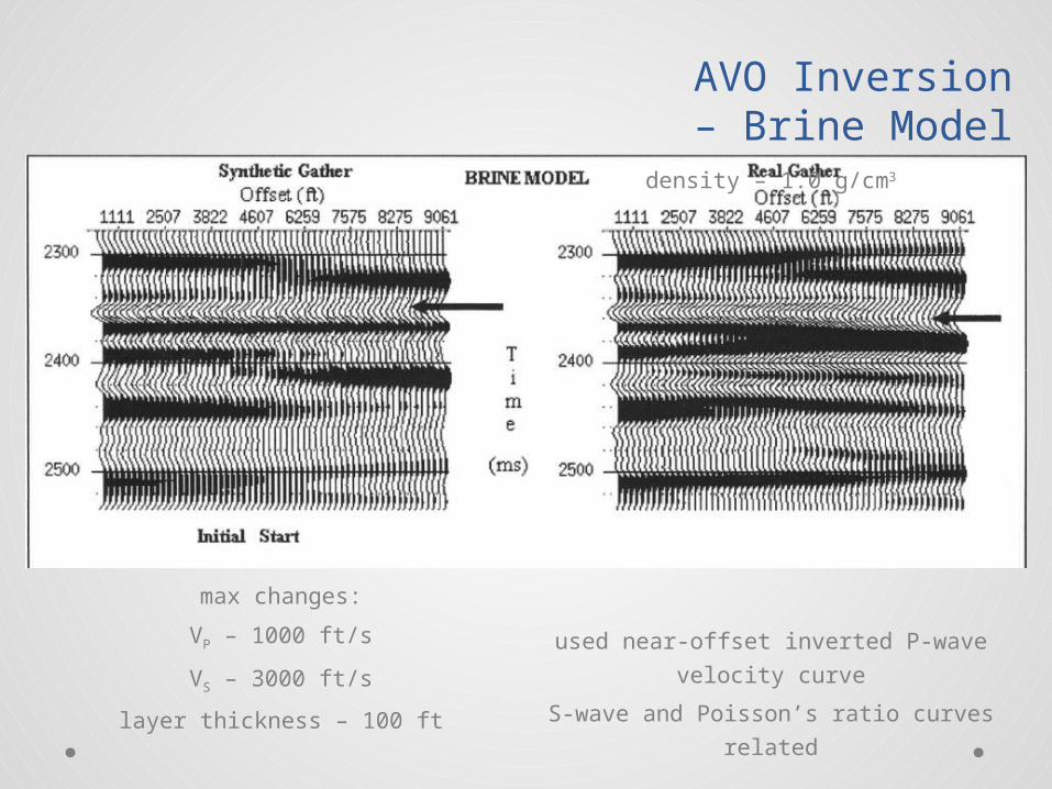
AVO Inversion – Brine Model

max changes:

VP – 1000 ft/s

VS – 3000 ft/s

layer thickness – 100 ft

density – 1.0 g/cm3

used near-offset inverted P-wave velocity

curve

S-wave and Poisson’s ratio curves related

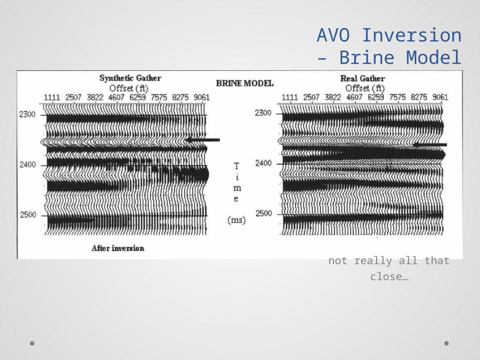
AVO Inversion – Brine Model

not really all that close…

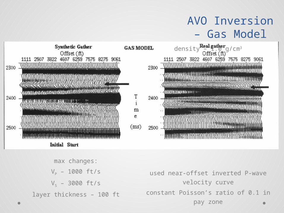
AVO Inversion – Gas Model

max changes:

VP – 1000 ft/s

VS – 3000 ft/s

layer thickness – 100 ft

density – 1.0 g/cm3

used near-offset inverted P-wave velocity

curve

constant Poisson’s ratio of 0.1 in pay

zone

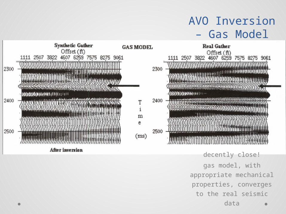
AVO Inversion – Gas Model

decently close!

gas model, with

appropriate mechanical

properties, converges to

the real seismic data

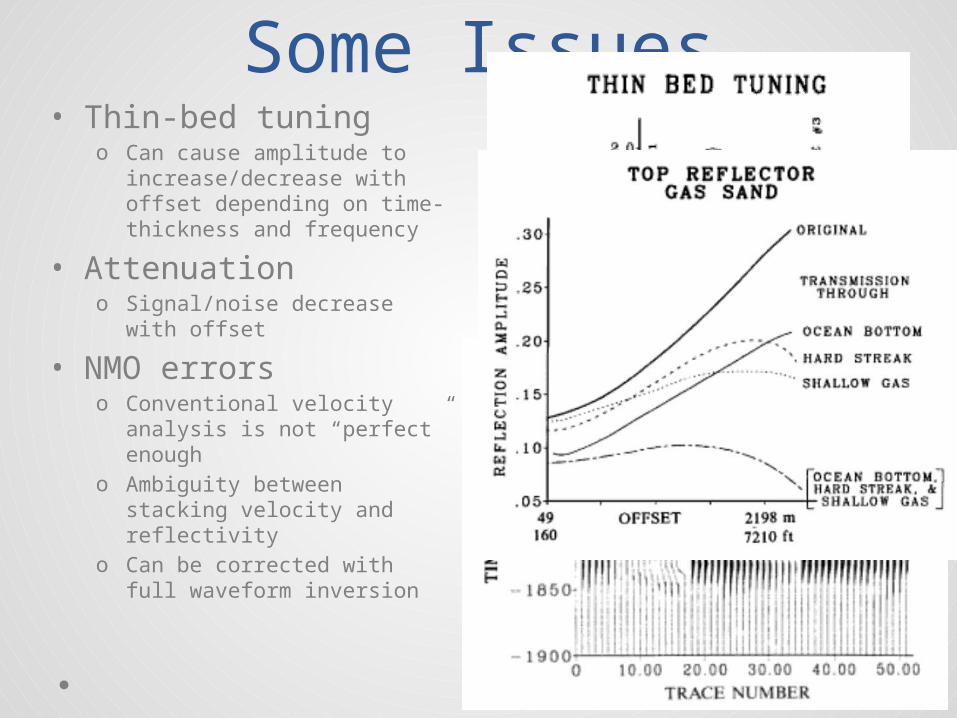
Some Issues• Thin-bed tuning

o Can cause amplitude to increase/decrease with offset depending on time-thickness and frequency

• Attenuationo Signal/noise decrease with

offset

• NMO errorso Conventional velocity analysis

is not “perfect” enougho Ambiguity between stacking

velocity and reflectivityo Can be corrected with full

waveform inversion

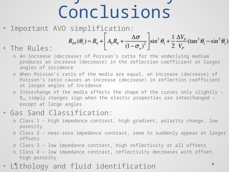
Key Takeaway Conclusions

• Important AVO simplification:

• The Rules:o An increase (decrease) of Poisson’s ratio for the underlying medium produces an

increase (decrease) in the reflection coefficient at larger angles of incidenceo When Poisson’s ratio of the media are equal, an increase (decrease) of Poisson’s

ratio causes an increase (decrease) in reflection coefficient at larger angles of incidence

o Interchange of the media affects the shape of the curves only slightly – RPP simply changes sign when the elastic properties are interchanged – except at large angles

• Gas Sand Classification:o Class 1 – high impedance contrast, high gradient, polarity change, low porosityo Class 2 – near-zero impedance contrast, seem to suddenly appear at larger

offsetso Class 3 – low impedance contrast, high reflectivity at all offsetso Class 4 – low impedance contrast, reflectivity decreases with offset, high

porosity

• Lithology and fluid identification

Key Takeaway Conclusions

References• Aki & Richards, 1980• Hilterman, 1983• Shuey, 1985• Smith and Gidlow, 1987• Hilterman, 1989• Koefoed, 1955• Ostrander, 1984• Rutherford & Williams, 1989• Castagna & Swan, 1997• Foster & Keys, 1999• Foster, Keys & Lane, 2010• Castagna, Swan & Foster, 1998• Nsoga Mahob, Castagna & Young, 1999• Fatti, Smith, Vail, Strauss & Levitt, 1994