ammonia-oxidizing bacterial community … bacterial community composition in estuarine and oceanic...

Ammonia-oxidizing bacterial community compositionin estuarine and oceanic environments assessed usinga functional gene microarray

Bess B. Ward,1* Damien Eveillard,2

Julie D. Kirshtein,3 Joshua D. Nelson,1

Mary A. Voytek3 and George A. Jackson2

1Department of Geosciences, Guyot Hall, PrincetonUniversity, Princeton, NJ, USA.2Department of Oceanography, Texas A and MUniversity, College Station, TX, USA.3USGS, Reston, VA, USA.

Summary

The relationship between environmental factors andfunctional gene diversity of ammonia-oxidizing bac-teria (AOB) was investigated across a transect fromthe freshwater portions of the Chesapeake Bay andChoptank River out into the Sargasso Sea. Oligo-nucleotide probes (70-bp) designed to represent thediversity of ammonia monooxygenase (amoA) genesfrom Chesapeake Bay clone libraries and cultivatedAOB were used to construct a glass slide microarray.Hybridization patterns among the probes in 14samples along the transect showed clear variations inamoA community composition. Probes representinguncultivated members of the Nitrosospira-like AOBdominated the probe signal, especially in the moremarine samples. Of the cultivated species, only Nitro-sospira briensis was detected at appreciable levels.Discrimination analysis of hybridization signalsdetected two guilds. Guild 1 was dominated by themarine Nitrosospira-like probe signal, and Guild 2�slargest contribution was from upper bay (freshwater)sediment probes. Principal components analysisshowed that Guild 1 was positively correlated withsalinity, temperature and chlorophyll a concentration,while Guild 2 was positively correlated with concen-trations of oxygen, dissolved organic carbon, andparticulate nitrogen and carbon, suggesting that dif-ferent amoA sequences represent organisms thatoccupy different ecological niches within theestuarine/marine environment. The trend from most

diversity of AOB in the upper estuary towards domi-nance of a single type in the polyhaline region of theBay is consistent with the declining importance ofAOB with increasing salinity, and with the idea thatAO-Archaea are the more important ammonia oxidiz-ers in the ocean.

Introduction

Nitrification is an essential link in the nitrogen cyclebetween organic matter decomposition (ammonification)and denitrification and subsequent removal of fixed Nfrom the system. The first step in the process is performedby ammonia-oxidizing bacteria (AOB) and archaea(AOA). Ammonia-oxidizing archaea are apparently thedominant group in the ocean (Wuchter et al., 2006) butthe relative abundance of AOB and AOA in estuaries hasnot been investigated. The AOB are phylogenetically con-strained to a few closely related groups in the gamma andbeta classes of the Proteobacteria. Although negativeresults are rarely reported, attempts to detect the gam-maproteobacterial AOB by polymerase chain reaction(PCR) are often not successful, implying that they are notvery abundant in seawater, despite their apparent special-ization on that environment.

At the 16S rRNA level, the betaproteobacterial AOB fallinto approximately 10 clusters (Purkhold et al., 2000). Thetwo largest clusters contain no closely related cultivatedmembers and are commonly detected in seawater. One ofthese is the uncultivated Nitrosospira cluster, whichappears to be the most important AOB in many marineenvironments; its members dominate clone libraries fromthe Mediterranean Sea (Phillips et al., 1999), polar seas(Bano and Hollibaugh, 2000; Hollibaugh et al., 2002) andMonterey Bay, CA (O’Mullan and Ward, 2005). Thesecond uncultivated marine cluster is more closely relatedto Nitrosomonas marina and Nitrosomonas oligotrophastrains and its members have been detected in the sameenvironments, generally as a smaller component of thoseclone libraries. The Nitrosomonas-like cluster is morelikely to be associated with particles (Phillips et al., 1999)and with higher ammonium concentrations (Kowalchukand Stephen, 2001) and dominates in some estuaries(Bollman and Laanbroek, 2002).

Received 12 October, 2006; accepted 9 May, 2007. *Forcorrespondence. E-mail [email protected]; Tel. (+1) 609 258 5150;Fax (+1) 609 258 0796.

Environmental Microbiology (2007) 9(10), 2522–2538 doi:10.1111/j.1462-2920.2007.01371.x

© 2007 The AuthorsJournal compilation © 2007 Society for Applied Microbiology and Blackwell Publishing Ltd

mailto:[email protected]

Investigations of AOB diversity have focused on boththe 16S rRNA gene and the signature functional gene,amoA (ammonia monooxygenase A) (Kowalchuk et al.,2000; Nicolaisen and Ramsing, 2002; Webster et al.,2002; Francis et al., 2003; O’Mullan and Ward, 2005;Freitag et al., 2006). O’Mullan and Ward (2005) detectedmuch greater sequence diversity at the amoA gene levelthan for 16S rRNA genes from similar sized clone librariesobtained from Monterey Bay. Two main groups corre-sponding to the two uncultivated 16S rRNA clusters wereidentified. The same two groups were found in YthanEstuary (Freitag et al., 2006) and in Chesapeake Baysediments (Francis et al., 2003), where several sub-groups were also detected.

The synthesis of previously published sequences fromcultures and environmental clone libraries enabledPurkhold and colleagues (2000) to associate the mainsequence clusters with gross environmental characteris-tics (e.g. seawater vs. soil), but this was a low resolutionanalysis, not based on quantitative analyses. Francis andcolleagues (2003) compared the level of amoA sequencediversity in clone libraries from Chesapeake Bay sedi-ments to the pairwise differences in environmental param-eters (e.g. salinity, oxygen, temperature, nitrate andammonium concentrations) between stations. Differencein salinity was the dominant variable and accounted for62% of the variation in pairwise sequence dissimilaritybetween stations. Ammonia concentration, the next mostimportant variable, explained only an additional 2.7%.Although AOA have not been investigated in estuaries, weexpect that their relative importance and abundance willincrease with salinity, opposite the trend for AOB.

Just as most investigations of diversity in the environ-ment have used the 16S rRNA gene to identify speciesand phylotypes, assessment of natural samples usingDNA microarrays has also exploited the 16S rRNAdatabase. Peplies and colleagues (Peplies et al., 2004)represented 18 16S rRNA phylotypes using short oligo-nucleotides on a DNA microarray, but were able to detectonly three groups by hybridizing with total RNA extractedfrom North Sea microbial communities. Functional groupshave also been targeted using 16S rRNA genes. Loy andcolleagues (Loy et al., 2004) used a hierarchical set of16S rRNA oligonucleotide probes to identify the majorsulfate reducing groups in acidic fen environments.Methanotrophs are analogous to the AOB in many ways,and they have been investigated in soils using short oli-gonucleotide DNA microarrays based on the particulatemethane monooxygenase gene (Bodrossy et al., 2003;2006; Stralis-Pavese et al., 2004). We previously demon-strated the approach with arrays containing multiple dif-ferent functional genes (nirS, nirK, nifH and amoA)(Taroncher-Oldenburg et al., 2003) and developed criteriafor probe design and data analysis.

The greater sequence divergence found in functionalgenes than in 16S rRNA genes from the same organisms(Purkhold et al., 2000) and the diversity patterns observedfor amoA in the Chesapeake system drove our focus onfunctional genes for array development. Here we usedDNA microarrays to investigate ecological signals in AOBamoA diversity in Chesapeake Bay (Fig. 1). By applyingthis approach in a system already characterized using theconventional clone library approach, we can compare theecological conclusions obtained from each, as well asevaluate the resolution and resources required for bothapproaches. In order to relate the amoA phylotype com-position to the environmental variables, we used a broadlyapplicable computational methodology for analysis of thediversity of microbial function in biogeochemical cyclesusing genetic data. This approach should also allow us tomake new conjectures about the mechanisms that controlthe distribution of the functional gene and of the functionalguilds that this diversity represents.

Results

Probe design

The phylogenetic relationships among the 24 probe70-mer oligonucleotides are represented in the tree(Fig. 2). The probe region corresponds to 449–518 bp inthe Nitrosospira briensis (NBU76553) sequence. Theprobes had an average melting temperature of81.3 � 2.7°C (Breslauer et al., 1986) and an average GCratio of 51 � 6 (Table S1, Supplementary material). The24 oligos include several clusters of sequences that arevery similar to each other (e.g. CT200d4 and CT200s1) aswell as single probes that are quite distant from all others(e.g. CBsed37 and CBsed12) (Fig. 2; Table S2, Supple-mentary material). Assuming that sequences within 85%identity of a probe will hybridize to that probe (Taroncher-Oldenburg et al., 2003), this probe set should capture theentire range of sequence diversity represented in theChesapeake Bay clone libraries. A gammaproteobacterialammonia oxidizer sequence from culture (Nitrosococcusoceani) was included in the probe set as a negativecontrol.

Array characterization

Probe resolution and specificity. Several experimentswere performed in which two targets were competitivelyhybridized in a label inverse design as previouslydescribed (Taroncher-Oldenburg et al., 2003). In everycase, the expected perfect match probe yielded the stron-gest hybridization signal, which in some cases wasmatched by the signal from probes with nearly identicalsequences. Related probes also hybridized significantly

amoA functional gene microarray 2523

© 2007 The AuthorsJournal compilation © 2007 Society for Applied Microbiology and Blackwell Publishing Ltd, Environmental Microbiology, 9, 2522–2538

(as defined by the results of signal filtering; see Experi-mental procedures and Fig. S1, Supplementary material).At the relatively high concentrations of target hybridized inthese experiments, some probes that were slightly lowerin identity than 85–87% (the identity level predicted toallow hybridization) did in fact produce significant signal(see Discussion).

The pattern of hybridization from various groups ofcompetitively hybridized probes was completely repro-ducible (2–4 replicate experiments for each probemixture) and indicated an identify cut-off of 80–85% forindependent probe resolution. Several ‘cluster probes’were thus identified, as groups of probes that cross react,i.e. that each hybridize with the same set of targetsequences. This analysis was consistent with the phylo-genetic analysis (Fig. 2) and reduced the effectivenumber of probes to those that are distinguishable byhybridization, i.e. have relatively low sequence identity.The total number of unique probes was thus reduced to14, including single probes Noceani, Nmestuarii, Nseuro,

Nmureae, Nmcryo, Nmmarina, CBsed1, CBsed12 andCBsed37, plus Cluster probes 1–5: Cluster probe 1 (i.e.the set of probes CBsed8, CBsed13, CBsed63); Clusterprobe 2 (CBsed10, CBsed26, CBsed61); Cluster probe 3(CT200s1, CB200d4, CB300s1, CB300s2); Cluster probe4 (Nsbriensis, Nstenuis, Nsmultiform); Cluster probe 5(Nmhalo, Nmoligo). The Nsbriensis probe sequence is infact more distant from the other members of its clusterthan the usual cut-off (78% vs. 80–85%); neither of theother two cultivated sequences in this cluster contributedsignificantly to the hybridization signal in environmentalsamples (see below), so it is convenient to group themwith Nsbriensis.

Probe capacity. Equal amounts of some targets yieldeddifferent fluorescence intensities even when hybridized totheir perfect match probes. Therefore, most of the probeswere tested independently to ascertain the scale of thisphenomenon, by comparing the fluorescence intensity ofthe perfect match hybridization (using the internal ratio

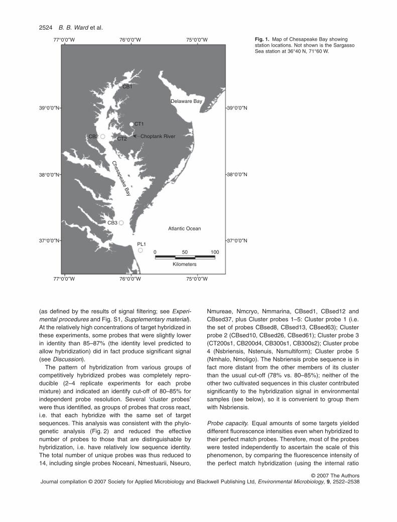
Fig. 1. Map of Chesapeake Bay showingstation locations. Not shown is the SargassoSea station at 36°40 N, 71°60 W.

76°0′0″W77°0′0″W 75°0′0″W

76°0′0″W77°0′0″W 75°0′0″W

39°0′0″N

38°0′0″N

37°0′0″N

39°0′0″N

38°0′0″N

37°0′0″NPL1

Atlantic Ocean

0 50 100

Kilometers

CB3

CB2 CT2

CT1

Choptank River

CB1

Delaware Bay

Chesapeake B

ay

2524 B. B. Ward et al.


method, summing the individual components of theCluster probes to treat each Cluster as one signal) withthat of the CBsed12 perfect match. Three of the probeswere not different from CBsed12, but four probes hadsignificantly less fluorescence and two significantly

greater (Fig. 3). Cluster probe 1 in particular had a fluo-rescence capacity 25-fold greater than that of CBsed12,i.e. 1 ng of one of the targets that hybridized with the fourprobes in Cluster probe 1 yielded 25 times greaterfluorescence intensity than did 1 ng of target CBsed12

Fig. 2. Distance tree (Clustal V, Higgins et al., 1991) based on the alignment of 24 70-mer oligonucleotide sequences on the amoA array. Thenumbered brackets indicate the groups of probes that comprise the five cluster probes.

Fig. 3. Differential fluorescence capacity of 100% perfect match target/probe combinations normalized to CBsed12 as 100% signal. Error barsrepresent standard deviation of results from multiple separate arrays.



hybridized with probe CBsed12. This dramatic differencehas serious implications for quantification of unknownmixtures (see below).

Results of array application to environmental samples

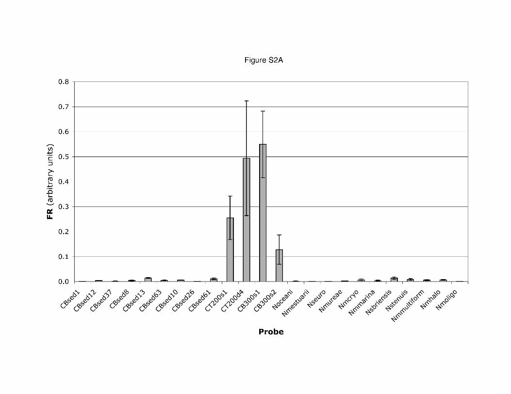
Hybridization data were determined for 14 water samplesusing the internal standard ratio method. Two examples,illustrating quite different hybridization patterns, areshown in Fig. S2 (Supplementary material). The coeffi-cient of variation (CV) for significant fluorescence ratio(FR) values averaged 30% across all slides. The largestCVs were associated with very low (insignificant) signals,which were observed frequently for features representingcultivated AOB sequences. Because the FR scale is notcalibrated and represents the average Cy3/Cy5 ratio foreach probe, the absolute FR scales cannot be compareddirectly between arrays. To assess the robustness of theindividual experiments, we analysed biological replicatesfor eight of the samples after completion of the originalanalyses. Duplicate filters that had remained frozen at-80°C since collection were extracted, labelled andhybridized using the same protocols as the original.Probes that yielded a hybridization signal � 5% of thetotal signal on each array were identified as present, anda similarity analysis using presence/absence data (Neiand Li, 1979) was performed. For the eight sets of dupli-cates, the similarity index [F = 2nxy(nx + ny)] ranged from50% to 100% and averaged 72% (SD 16%). The maindifference between replicates was that the first set ofexperiments detected more significant signals than thelater ones; in only one sample did the later experimentdetect one signal that was not present in the first set. Thiswas attributed to degradation of the arrays – the replicateexperiments were performed 2.5 years after the initialexperiments.

Relative FR values were used to compare hybridizationpatterns among different samples (Fig. 4A). The sameamount of total target (100 ng) was hybridized with eacharray, so the proportion of signal attributed to each probeis the appropriate comparison. The largest signals wereobserved for amoA probes derived from a group of closelyrelated clones: CB300s2, CB300s1, CT200d4 andCT200s1. This group, identified as Cluster probe 3 above,constituted 4.6–93.7% of the total signal in the 14samples. Its highest contributions (91.7%, 93.5% and93.7%) occurred at CT200D, PL100D and CB200D, alldeep water samples from the river, plume and bayrespectively. Its smallest contributions (4.6%, 28.2% and34.5%) occurred at CB100D, PL100M and SS100S, deepwater from the upper bay and mid and surface watersamples from the plume and Sargasso Sea respectively.Cluster probe 3 represented on the order of 50% of thetotal signal in all other samples.

Probes CBsed8, CBsed13 and CBsed63 (identified asCluster probe 1 above) were the next most importantgroup in magnitude of the hybridization signal, accountingfor almost half the total signal at CB200S and close to40% at CB300D.

The 11 individual probe sequences representing culti-vated strains were consistently among the lowest signals,frequently being in the background (Fig. 4A). The indi-vidual probe representing N. briensis (Nsbriensis, identi-fied as part of Cluster probe 4 above) produced thehighest signal among the cultivated strains. Cluster probe4 represented up to 28.9% of the total signal (sampleCB100D), but was usually less than 5% and often lessthan 1% of the total. The only other cultivated sequencerepresented significantly in the hybridization signal wasNitrosomonas cryotolerans (Nmcryo), which reached8.2% of the total signal in SS100M. It is clear from thecapacity tests, however, that the fluorescence signalscannot be interpreted quantitatively in terms of targetabundance in the sample (see Discussion).

Analysis of probe resolution

Relative FR results for all individual probes were sub-jected to discrimination to identify probes that tended tobehave similarly in the hybridizations with environmentalsamples. This initial analysis identified groups of probesthat did not behave independently because they hybrid-ized to the same targets – the Cluster probes identifiedabove. The phylogenetic analysis of sequence compari-sons, the simple mixture experiments and the probebehaviour in hybridization experiments with environmen-tal samples were all consistent with each other, andestablished a distance criterion slightly larger than15 � 3% criterion established with the earlier arrays(Taroncher-Oldenburg et al., 2003) for resolution of dis-tinct genotypes.

In the experiments with environmental samples, thetendency of the probes to cross react cannot be distin-guished from the potential co-occurrence of differenttargets (correlation in the signal intensity because thedifferent targets have similar distributions in the samples).The fact that the hybridization results from environmentalsamples were consistent with the phylogenetic analysisand the simple mixtures (i.e. all probes within each Clustershowed similar hybridization patterns, essentially actingas a single probe), however, indicates that the compo-nents of the Cluster probes detected the same targets,rather than correlated occurrences of unrelated targets.For example, the four probes (CT200d4, CT200s1,CB300s1 and CB200s2), which consistently yielded thehighest signal in most samples, were 82.9% – 95.7%identical to each other (Table S2, Supplementary mate-rial) and were identified as Cluster probe 3 above. Targets



A

B

Fig. 4. Composite bar plot showing relative FR for all probes (A) and for the 14 independent probes (B) in all samples. The total FR signalswere summed and the FR value for each probe is represented by its fraction of the total signal. The first station on the x-axis is the onlyChoptank River station, CT200, from a location with intermediate salinity. The other stations are arranged beginning with the freshwater upperstation in the Bay (CB100) in order of increasing salinity towards the open ocean station, SS100.



that hybridize with one of the four should in fact hybridizewith all of them (Fig. S1, Supplementary material), and itis clear from the bar plot that these four probes did indeedbehave similarly across the sample set (Fig. 4A). In con-trast, the Nmestuarii probe was 88.6% identical to bothCBsed13 and CBsed63, but only 82.9% identical toCBsed8. Although the three sediment clones exhibitedstrong hybridization signals, Nmestuarii never reached1% of the total signal strength, so it was not considered amember of Cluster probe 1.

When the relative FR values for individual probes withineach Cluster probe were summed, treating each Clusterprobe as one signal, the patterns of the 14 independentprobes (nine single probes and five Cluster probes)(Fig. 4B) emphasize the dominance of Cluster probes 1, 2and 3 in the overall distribution.

Analyses of hybridization patterns inenvironmental context

Due to the large variability of the data and the variability inprobe capacity, we did not use fluorescence intensity

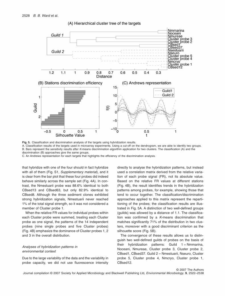
directly to analyse the hybridization patterns, but insteadused a correlation matrix derived from the relative varia-tion of each probe signal (FR), not its absolute value.Based on the relative FR values at different stations(Fig. 4B), the result identifies trends in the hybridizationpatterns among probes, for example, showing those thattend to occur together. The classification/discriminationapproaches applied to this matrix represent the reparti-tioning of the probes; the classification results are illus-trated in Fig. 5A. A distinction of two well-defined groups(guilds) was allowed by a distance of 1.1. The classifica-tion was confirmed by a K-means discrimination thatmatches significantly 71% of the distribution in two clus-ters, moreover with a good discriminant criterion as thesilhouette score (Fig. 5B).

The convergence of these results allows us to distin-guish two well-defined guilds of probes on the basis oftheir hybridization patterns: Guild 1 = Nmmarina,Noceani, Nmureae, Cluster probe 3, Cluster probe 2,CBsed1, CBsed37. Guild 2 = Nmestuarii, Nseuro, Clusterprobe 5, Cluster probe 4, Nmcryo, Cluster probe 1,CBsed12.

Fig. 5. Classification and discrimination analysis of the targets using hybridization results.A. Classification results of the targets used in microarray experiments. Using a cut-off on the dendrogram, we are able to identify two groups.B. Bars represent the sensitivity results after K-means discrimination algorithm application for two clusters. The classification (A) and thediscrimination (B) approaches give the same groups.C. An Andrews representation for each targets that highlights the efficiency of the discrimination analysis.



The Andrews representation (Fig. 5C) summarizesthese multivariate data and the related guilds. The repre-sentation indicates similar frequency for both guild curves,which means that both guilds exhibit the same qualitativevariation in the function of the stations. However, theamplitudes of the guild signals are different which impliesthat the probes exhibit different hybridization intensities asa function of station (i.e. environmental conditions). Weinterpret these results to imply that the hybridization pat-terns reflect variation in the distribution of the functionalgene amoA, which is related to the ecophysiology ofammonia-oxidizing microorganisms. Thus, relative FRpatterns reflect the variation in biological function relatedto organisms that possess amoA.

The guilds defined on the basis of relative FR in anenvironmental context constitute functional groups, whichsuggests some ecological significance of the hybridizationpatterns. Guild 1 contains mostly marine sequences (e.g.Nmmarina, Nmureae), and its signal is dominated byCluster probe 3, which contains sequences derived fromthe water column at stations CB200 and CB300. Guild 2includes the obviously freshwater AOB sequences (e.g.Nseuro and Cluster probe 4) and Cluster probe 1 (com-posed of sequences from CB100 sediments) is a maincomponent of its signal. The signal from the cultivatedstrains was so low that to base the guild characteristics onthem is not warranted. The ecological and physiologicalcharacteristics associated with organisms from which thesequences in Cluster probes 1, 2 and 3 were derivedcannot be known a priori, but phylogenetic affiliations andsubsequent analysis suggests that Cluster probe 3represents the main marine planktonic Nitrosospira-likegroup and Cluster probe 1 represents an importantNitrosomonas-like group from freshwater sediments. Thisobservation suggests some relationship between thehybridization results and the physical characteristics ofthe environment at the various stations.

Projection of the functional guilds into physicalparameter space

These two guilds are composed of targets that tend toco-occur in the samples, and may represent two amoAcommunities with different ecophysiological characteris-tics and different geographical distributions, likely relatedto environmental conditions. The corresponding physicaland chemical parameters for each sample were includedin a correlation based principal components analysis(PCA) with the hybridization signals for the two guildsrepresented by the 14 independent probes (Fig. 6). Thefirst and second components represent 74% and 10.8%,respectively, of the global variability in the data set. Guild1 was positively correlated with salinity, temperature andchlorophyll concentration and negatively with most of the

other variables. Guild 2 was positively correlated withoxygen, particulate nitrogen, particulate carbon and dis-solved organic carbon. In the same feature space, thecentroid of both guilds indicates an antagonistic relation-ship to urea, nitrite, dissolved organic nitrogen, silicate,dissolved organic phosphate and dissolved amino acids,which implies at least a non-linear effect of these param-eters on the global amoA community.

Community composition as a function of station

One major goal of the microarray experiments is to allowcomparison of microbial community composition amongstations. Thus, a classification/discrimination approachsimilar to that described above was applied to the stationsin order to classify or group them according to their hybrid-ization patterns (Fig. 7A). A distinction of two clusters wasallowed for 1.1 distance cut-off and a posteriori confirmedby a K-means approach for two clusters (cf. correspond-ing silhouette score for each station in Fig. 7B) and anAndrews representation (Fig. 7C). Thus, two main groupsof stations were distinguished:

Station group 1: CB100S, CB200S, PL100S, CB300D,CB300S. Station group 2: SS100M, PL100M, PL100D,CB200D, CB100D, CB100M, SS100S, CB300M,CT200D.

Fig. 6. Projection of the variables in the first component featurespace in the principal components analysis. The first and thesecond component represent 74% and 10.8% of the globalvariability respectively. The bold variables correspond to the twoguilds identified from the microarray hybridization patterns. Symbolsrepresent salinity (S), temperature °C (T) and concentrations ofoxygen (O2), particulate nitrogen (PN), dissolved organic carbon(DOC), particulate carbon (PC), ammonium (NH4), orthophosphate(oPhos), nitrate (NO3), total dissolved nitrogen (TDN), ratio ofparticulate carbon/particulate nitrogen (PCPN), total dissolvedphosphate (TCP), dissolved organic phosphate (DOP), dissolvedfree amino acids (DFAA), silicate (Si), dissolved organic nitrogen(DON), nitrite (NO2), urea (Urea) and chlorophyll a (Chl).



A classification of these stations according to physicaland chemical parameters only was attempted. The dis-crimination efficiency for stations was less relevant androbust, however, than the guild discrimination. Moreover,using the available data, the physical and biological dis-tributions are not significantly identical (55% identical), i.e.classifying the stations according to physical/chemicalpatterns results in different groups than when classifyingthem by hybridization pattern in 45% of the 10 000 itera-tions of the discrimination calculation.

Discussion

Interpretation of environmental microarray data

The microarray approach depends first on the develop-ment of an adequate sequence database, in order torepresent on the array the full range of sequence diversitylikely to be encountered in the environment (Francis et al.,2003; Stralis-Pavese et al., 2004), although comparisonsamong large numbers of samples on the basis of exhaus-

tive clone libraries is prohibitive in time and expense. Dueto their high throughput capabilities, microarrays havegreat potential for ‘fingerprinting’ microbial communities atboth the DNA and RNA level for presence/absence anddiversity information. There are two main issues, however,that preclude more quantitative interpretation of the arraydata at present.

Probe specificity. The ability of the individual probes toresolve closely related sequences is limited and variable(Marcelino et al., 2006), but for 70-mers and PCR prod-ucts in various hybridization formats is about 15%sequence identity (Kane et al., 2000; Taroncher-Oldenburg et al., 2003; Steward et al., 2004). The two-colour competitive hybridization and the internal standardratio hybridization methods showed comparable resolu-tion in terms of target binding specificity. The heterologousprobes most likely to hybridize at increased target con-centration were robustly predictable on the basis of thephylogenetic tree shown in Fig. 1 – e.g. Nmestuarii is on

Fig. 7. Classification analysis of stations grouped by hybridization pattern.A. Classification result of the stations based on hybridization results. Using a cut-off on the dendrogram, we are able to identify two groups.B. Bars represent the sensitivity results after K-means discrimination algorithm application for two clusters. The classification anddiscrimination approaches give the same groups.C. An Andrews representation for each station that highlights the efficiency of the discrimination analysis.



the outer edge of the cluster containing CBsed8,CBsed13 and CBsed63, which all cross react stronglywith each other. At the target concentrations used forenvironmental samples, it is unlikely that any individualtarget reached levels (~25 ng) at which significant crosshybridization was observed in the specificity tests. Thus,cross reaction among probes that differ by � 15% isunlikely in environmental experiments.

The degree of cross hybridization depends on thebinding free energy of the probe/target hybrid molecule aswell as the degree of sequence identity. Mismatchedtarget/probe molecules generally hybridize at target con-centrations less than 5 ng if the mismatched hybrid mol-ecule has a calculated binding free energy � 56% of thebinding free energy of the perfect match target/probehybrid (Taroncher-Oldenburg et al., 2003), althoughexceptions occur. For example, CB300s1 and CB200d4are 84.3% identical and have binding free energy for thehybrid molecule of 45% of the CT200d4 perfect match.Nevertheless, CB300s1 hybridized consistently in simplemixtures (e.g. Fig. S1, Supplementary material) and infield samples as if it were indistinguishable from the othermembers of Cluster probe 3. Because the simple mixtureresults confirm that CB300s1 belongs in this cluster, wediscount the possibility that the field data representhybridization with an independent sequence that simplycovaries with the other members of Cluster probe 3.

Nmestuarii, on the other hand, is 88.6% identical toCBsed8 and has a binding free energy equivalent to49.9% of the CBsed8 perfect match. Although the Nmes-tuarii probe yielded significant signal in the simple mixturetest such that it behaved like a member of Cluster probe1, Nmestuarii never hybridized at a significant level in fieldsamples. Apparently the targets from the natural samplesthat hybridized with the probes that comprised Clusterprobe 1 were distinct from Nmestuarii.

Despite these constraints, the degree of resolutionoffered by the array hybridizations is still relatively highand is sufficient to be ecologically informative. Ammonia-oxidizing bacteria differ at the 16S rRNA gene level byless than 10% over the whole gene (Purkhold et al.,2003), and the amount of variation in the most commonlystudied 490 bp fragment of the amoA gene is on the orderof 25% (Francis et al., 2003). By selecting a highly vari-able 70-mer region from within the amoA fragment, thearray probe sequences differ by as much as 70%, vastlyincreasing the power to distinguish among types. Theminimum probe resolution for the 14 independent probesused here was about 15%, which corresponds roughly tothe species cut off of 2–3% at the 16S rRNA level.Purkhold and colleagues (2000) compared the 16S rRNAand amoA similarities from cultured AOB strains, andfound that a 3% 16S rRNA distance equates to a 15%amoA distance. Similar patterns were observed in corre-

lated shifts of paired environmental samples using analy-ses of AOB-specific 16S rRNA similarity compared withamoA similarity (O’Mullan and Ward, 2005). Thus, thearray resolves amoA community composition at an eco-logically relevant level.

Probe capacity. Differential fluorescence intensity amongperfect match probe/target combinations has not beenwidely considered as a factor in the interpretation of arrayhybridization data in environmental studies. Using shortoligonucleotide probes on a tiling array, and hybridizing torRNA targets from microbial eukaryotes, it was concludedthat hybridization intensity cannot be predicted from ther-modynamic calculations based on probe sequence andmismatch characteristics (Pozhitkov et al., 2006), andsuggested this may be due to the inability of thermody-namic calculations to explain the behaviour of the surface-bound probe molecule interacting with the soluble target.While it is not practical to evaluate each individual probeon arrays containing hundreds or thousands of features,for the small probe set used here, it was practical to testmost probes separately or in non-cross reacting mixtures(Fig. 3). If the extreme case of Cluster 1, for which onlyone experiment is available, is excluded, the range ofrelative fluorescence capacity for different perfect matchprobes is > 10-fold (0.14–1.8 for CBsed1 and CBsed37respectively) relative to CBsed12. Full length (~1500 bp)16S rDNA probes hybridized with 18–21-mer oligonucle-otide probes exhibited capacity differences of at leastsevenfold for perfect match probe/target hybrids and up tonearly 200-fold for probes with small but similar levels ofmismatch (Sanguin et al., 2006). Pozhitkov and col-leagues (2006) reported intensity variations amongperfect match probes of 70-fold that could not beexplained by thermodynamic or sequence characteristics.Some of the variability in capacity may be explained bydifference in melting temperature; for the probes testedhere, the fluorescence capacity generally decreased asmelting temperature increased. Sanguin and colleagues(2006) reported the same tendency, but also noted unex-plained examples of complete failure of hybridization forcertain locations in the amplicon, even for probes target-ing perfect match sequences. Steric hindrance of longPCR products or loss of target to competitive rehybridiza-tion with the complementary strand of the PCR productmay explain part of capacity variability. However, theseissues were minimized in our protocol because the targetitself was a Klenow-labelled product, i.e. a mixture offragments < 450 bp in length, and the mixture should havebeen random and similar among target preparations.

The net effect of both of these issues is to introduceunknown variation into the relationship between targetabundance and hybridization fluorescence intensity. Bothresolution and capacity can be quantified and corrected



for in known mixtures, but not for unknown mixtures, e.g.environmental samples. Because of the thermodynamicunpredictability of hybridization, we cannot assume thatall targets that hybridize with a certain probe (perfectmatch targets plus mismatch targets with up to ~15%identity differences) will exhibit the same capacity, andthus we cannot simply apply the capacity correction thatwas determined for the perfect match hybridization tounknown mixtures. Therefore, the ecological analysespresented here were not based on absolute fluorescenceintensity. amoA occurs in multiple copies in most AOB (upto three copies in cultivated strains; Norton et al., 2002),which introduces further variability in the relationshipbetween hybridization intensity and AOB abundance.Even given these limitations for quantification, strikingpatterns emerged in the distribution of positivehybridization.

Ammonia-oxidizing bacteria community composition

The range of amoA diversity represented on the arrayfocused on sequences represented in clone libraries fromthe water column and sediments of the Chesapeakesystem, but included sequences representing most, butnot all, of the cultivated species/strains. The most strikingresult of the hybridization patterns is that the signalstrength for the cultivated strains was much lower than formost of the environmental sequences. The target popu-lations were produced by PCR amplification usingbetaproteobacteria-specific amoA primers. Therefore,Noceani should not have been represented in the targetmixture and no signal was ever detected with the Noceaniprobe. All of the other cultivated strain probes, however,represent species that can be easily amplified with theseprimers. Nsbriensis was the only probe from a cultivatedstrain that hybridized to any extent and it was most impor-tant in the deep sample from the most freshwater station(Fig. 4A). This probably represents an influence from thesurrounding terrestrial environment and indicates theorganisms with amoA sequences very similar to N. brien-sis may be important in that environment. The capacity ofCluster 4, which included Nsbriensis, was only 27% ofCBsed12, so its contribution is underestimated in Fig. 4B,but even if it were possible to correct for capacity, Cluster4 would still be a minor component of the other samples.

The strongest hybridization was observed with probesrepresenting Cluster probe 3, a group within the unculti-vated marine Nitrosospira-like sequences in the overallamoA phylogeny. The reproducible and widespreadstrong detection of this group is consistent with thegroup’s previously implied importance in the marine envi-ronment on the basis of clone libraries. The relative con-tribution of Cluster probe 3 was often more than 50%, ofthe total signal. The lowest value was observed in the

deep water sample from the upper Chesapeake Bay,where Nsbriensis was an important signal. This upper baysample was one of the least marine in character, and thedeep water composition may reflect a community of fresh-water sediments unlike that in the upper water column ofthe larger Bay environment. With a fluorescence capacityof 60% relative to CBsed12, Cluster 3 would be under-represented in Fig. 4B, making its contribution even moreoverwhelming in many of the samples.

The high fluorescence capacity of Cluster 1 implies thatits contribution to the target composition is overrepre-sented in Fig. 4B. The single probe CBsed12 exceeded30% of the total signal in the Sargasso Sea surfacesample. None of these sequences are associated withcultivated strains, but all represent members of theNitrosospira-like and Nitrosomonas-like clades, respec-tively, that are frequently reported as major components of16S rRNA and amoA clone libraries from marine sites(Bano and Hollibaugh, 2000; Freitag and Prosser, 2004;O’Mullan and Ward, 2005). Cluster probe 3 was identifiedas a component of Guild 1, while both Cluster probe 1 andCBsed12 were part of Guild 2, suggesting that the organ-isms represented by these sequences may representecologically distinct niches.

Ecological significance of guilds

The amoA array as described here was used to detectDNA directly. It thus provides an indication of the relativeabundance and diversity of different amoA phylotypes, asreflected in pooled PCR products, at the level of geneticcapability for ammonia oxidation. Visual inspection of thehybridization patterns (Fig. 4B) reveals obvious groups ofstations: CT200D, CB200D, PL100D and SS100M wereall dominated by Guild 1, especially Cluster probe 3.CB100S, CB100D, CB200S, CB300S, CB300M,CB300D, PL100S, PL100M and SS100S all showed animportant contribution from Guild 2, mostly due to Clusterprobe 1 (Nitrosomonas-like sequences) and CBsed12.Clear biogeographic patterns emerged in the identificationof the two guilds and their relationship to environmentalvariables (Figs 5 and 6).

The classification of stations on the basis of phylotypepatterns (Fig. 7) is, however, significantly different fromthe classification of stations on the basis of physical andchemical variables. That is, some stations with similarenvironmental characteristics differ in amoA communitycomposition. Thus, it is not possible to identify completelythe environmental variables that determine the biogeo-graphical patterns evident in the hybridization data.

The next step in the application of microarray technol-ogy to understanding biogeochemical processes in theenvironment is to assess gene expression by hybridizingwith mRNA or cDNA derived from environmental samples.



RNA/cDNA might reflect short time scale changes but dueto the slow growth rate of AOB, DNA may be a betterreflection of AOB response on the time scale of environ-mental variability in the bay. That is, highly abundant typesmust be successful in the environment as integrated overthe timescale of the last few bacterial lifetimes. Methan-otrophs are analogous to AOB in many ways, and similarmethodology has recently been used to investigate thecommunity composition of methanotrophs under variouslandfill and vegetation conditions (Stralis-Pavese et al.,2004). This study used a very different microarrayapproach (Bodrossy et al., 2003), in which short oligos(18–24-mers) and competitive two-colour methodologywere employed. Stralis-Pavese and colleagues (2004)were able to identify the dominant methanotrophs at theDNA level and to identify different groups associated withdifferent experimental conditions. Using RNA targets(Bodrossy et al., 2006), the same major groups wereidentified, but RNA was detected for some groups notdetected at the DNA level – groups that must haveresponded particularly well to current conditions.

Ecology of AOB in estuarine environments

Salinity appears to be a major environmental selectionfactor for estuarine microbial communities, both for thetotal community (Bouvier and del Giorgio, 2002; delGiorgio and Bouvier, 2002) and for AOB assemblages inparticular (Bianchi et al., 1999; de Bie et al., 2001; Bern-hard et al., 2005). Microbial community composition(Bouvier and del Giorgio, 2002) and cellular activity (delGiorgio and Bouvier, 2002) both varied dramatically in thegradient from freshwater in the upper Choptank River tothe moderately saline (14 psu) region where the Chop-tank joins Chesapeake Bay. Betaproteobacteria were thedominant bacterial clade in the freshwater environmentand were replaced by alphaproteobacteria at the highersalinity stations. The greatest change occurred between 4and 8 psu in the salinity gradient. Cottrell and Kirchman(Cottrell and Kirchman, 2004) documented the samecommunity composition changes in the Delaware estuary.

Large shifts in the composition of 16S rRNA and amoAclone libraries representing AOB communities have beenreported for the Schelde estuary in the Netherlands (deBie et al., 2001; Bollman and Laanbroek, 2002), WaquoitBay in the US (Bernhard et al., 2005), and ChesapeakeBay as an initial step in our study of amoA functionaldiversity in this system (Francis et al., 2003). amoA clonelibraries (Francis et al., 2003) from the same CB and CTstations investigated here showed the greatest composi-tional differences between the upper bay (CB100) andupper river (CT100) stations compared with all the rest.On the basis of visual inspection of the hybridization pat-terns (Fig. 4B), the three freshwater samples (station

CB100) were quite different from most other samples,likely representing the freshwater end member of the AOBcommunity. The fact that CB200S (but not the otherCB200 samples) was very similar to CB100S probablyreflects the fact that surface water at CB200 originates inthe freshwater region of CB100, while the deeper samplesrepresent the deep water brought in from the mouth of thebay by the usual estuarine circulation. CT100 was notsampled for the present study, but CB100 was differentfrom many of the other stations in its lower contribution byGuild 1 (Cluster probe 3) and the greater importance ofmembers of Guild 2. At CB200 and CB300, the freshwatersediment Guild 2 was well represented in the surfacesamples, which was also important in the deep samplefrom CB300. CB200D and CB200D were both dominatedby Guild 1, consistent with the seawater wedge of theestuary extending further north in the deep water than atthe surface. Thus, the microarray results and clone librarydata are consistent in both their descriptions of the com-munity and the ecological implications of variations incommunity composition, validating the microarrayapproach for high throughput investigations of communitycomposition and diversity.

Salinity variations are not important in the ocean, atleast nowhere near the scale of variability found inestuaries. Nevertheless, both major clades, Nitrosospira-and Nitrosomonas-like, are found in seawater, showingsmall-scale spatial and temporal variability (O’Mullan andWard, 2005). It now appears that the AOA dominate theammonia oxidizing community of the open ocean(Wuchter et al., 2006). The trend from high diversity to lowin the AOB along the estuarine gradient is consistent withthe idea that AOB are not very important in the ocean.Only a few types are capable of living in full strengthseawater, and even those are not abundant. A similarstudy of AOA along the estuarine gradient might beexpected to yield the opposite pattern.

Experimental procedures

Study site

The Chesapeake Bay drains a watershed of 166 000 km2 andfills a dendritic river valley system consisting of a mainchannel and seven main rivers, including the Choptank River,a subestuary that contributes about 1% of the total freshwaterto the bay. Six stations (Fig. 1) were chosen to span a rangeof environmental conditions; their characteristics have beendescribed previously by Francis and colleagues (2003), whodescribed the diversity of amoA clone libraries from thissystem. Characteristics of the depths sampled in April 2002are provided in Table 1.

Sample collection and DNA extraction

The water column (two or three depths) was sampled in April2001 and April 2002 using a pump in the river and Niskin



bottles on a CTD rosette in the bay, plume and Sargasso Sea.Samples collected in April 2001 were used to construct theclone library and samples collected in April 2002 were used inthe array hybridization experiments. Water samples werecollected from surface, mid depth and deep water, defined bythe relative depth at each station: surface was generally 1 m,deep was 1 m off the bottom (except in the plume and theSargasso Sea) and mid was in between, often chosen tosample a stratification feature such as the bottom of thethermocline or a particle maximum feature. Surface sedi-ments were collected at the North Bay site (CB100) in April2001 using a box core. A few grams of surface sediment weresubcored using a cut-off plastic syringe, then scraped into asmall tube and immediately frozen in liquid nitrogen. Sampleswere stored at -80°C until DNA extraction.

Particulate material from the water samples was collectedby peristaltic pump filtration onto Sterivex GP 0.2 mm filtercapsules (Millipore, Billerica, MA), which were drained,capped and frozen in liquid nitrogen immediately uponcollection. DNA was extracted from the capsules using thePureGene DNA kit with slight modification of manufacturer’sprotocol for extraction of Gram negative bacteria (Gentra,Minneapolis, MN): lysis buffer (0.9 ml) was added to the filterand incubated with gentle rotation for 10 min at 80°C. Incu-bation times for all subsequent steps were the maximumrecommended. Sediment DNA was extracted according tomanufacturers instructions using the Ultraclean soil DNA kit(MoBio Laboratories, Carlsbad, CA).

Polymerase chain reaction, cloning, RFLP screeningand sequencing

A fragment of the amoA gene was amplified from environ-mental samples and pure culture extracts using the betapro-teobacterial amoA primers and PCR conditions of Rotthauweand colleagues (Rotthauwe et al., 1997). Amplicons werepurified by Wizard PCR prep (Promega, Madison, WI) andcloned into pCR2.1 vector using the Topo TA Cloning kit(Invitrogen, Carlsbad, CA). Transformants were screened forinserts by PCR using the amoA primers. At least 48 positive

amoA amplicons from each sample were digested withSau3A and HinfI for 3–6 h at 37°C to assess diversity of thecloned sequences. Digests were electrophoresed on a 3%Methaphor agarose gel (FMC BioProducts, Rockland, ME,USA) at 60 V, stained and photographed. Several represen-tatives of each RFLP pattern type were then sequenced inboth directions using amoA primers and Big Dye 3.1, accord-ing to manufacturers instructions (Applied Biosystems,Foster City, CA). Sequencing was performed on the ABI310genetic analyzer.

Microarray oligonucleotide probe design

Rather than including every known sequence as a probe onthe array, we chose a subset designed to represent the wholerange of diversity with minimal cross reactivity among probes.Sequences from the April 2001 data set (surface and deepwater samples from CB200, surface and deep water samplesfrom CB300, and CB100 sediment) were locally aligned witheach other and with other environmental and culture-basedamoA sequences available in GenBank (NCBI). Phylogenetictrees were built using PAUP v 4.0 both for the total fragment(approximately 400 bp) and for several possible 70 bpstretches of sequence to find areas of the gene with thehighest sequence dissimilarity that still represented the phy-logenetic relationships visualized in the whole fragmentphylogeny. Based on this comparison, 24 oligos werechosen, 13 from our environmental amoA sequences and 11additional culture-based sequences (Table S1, Supplemen-tary material). Nitrosomonas eutropha and Nitrosomonaseuropaea sequences are identical over the probe region, sothe probe called Nseuro represents them both. Three culti-vated sequences (Nitrosococcus mobilis, Nitrosomonas com-munis and Nitrosomonas nitrosa) have been detected rarelyif at all in our clone libraries and were not available for testingso they were not included on the array. The original clonelibrary survey was performed using betaproteobacteria-specific amoA primers and the same primers were used toproduce target for the hybridization experiments (see nextsection). The 70-mer oligo probes (Operon Technologies)

Table 1. Station locations and characteristics (data from April 2002).

Station Depth (m) T (°C) Salinity Nitrate (mM) Chlorophyll a (mg l-1) Sediment type

CT200D 7 ND ND 0.03 4.79 MudCB100S 1.9 9.9 0.1 59.1 1.27CB100M 4 9.8 0.1 ND NDCB100D 7.8 9.8 0.1 58.1 1.49 MudCB200S 2 9.9 15.1 4.5 8.53CB200D 19 9.0 21.1 0.4 8.81 MudCB300S 1.9 11.4 24.5 0.14 3.93CB300M 7.5 11.4 25.8 ND NDCB300D 9.2 11.7 25.9 0.64 4.39 Sand/mudPL100S 1 12.5 29.2 0.04 2.57PL100M 6.5 11.8 27.8 ND NDPL100D 12.5 11.6 32.8 0.68 2.12 NASS100S 1 20.4 36.4 0.15 0.22SS100M 100 19.5 ND 0.10 0.23

The temperature and salinity data were provided by W. Boicourt and the nutrient data were provided by P.M. Glibert, both of Horn Point Laboratory,University of Maryland Center for Environmental Sciences.T, temperature; ND, not determined; NA, not applicable.



were adjusted to a concentration of 0.05 mg ml-1 in 50%DMSO and were spotted on CMT-GAPS amino silane-coatedglass slides (Corning, Corning, NY). After printing, the slideswere baked at 80°C for 3 h and stored in the dark at roomtemperature under slight vacuum.

Hybridization experimental design

Two different protocols were used: (i) the standard two-colourcompetitive approach was used for the initial array testingand (ii) a new internal standard ratio method was used for theanalysis of environmental samples and for capacity tests. Thestandard two-colour competitive hybridization method wasused previously to establish hybridization criteria for func-tional gene oligonucleotide arrays (Taroncher-Oldenburget al., 2003). It was used here to characterize the behaviourof the amoA array in simple defined mixture experiments inorder to verify the criteria established previously in a differentgene system. The competitive hybridization approach wasnot appropriate for the actual analysis of field samples,however, because it is difficult to define a true ‘control’ sampleor a ‘normal’ sample against which all others should be com-pared, as is the case for gene expression in diseased tissueversus healthy tissue, for example. One of the major advan-tages of the competitive approach, however, is the use ofFRs, rather than simple hybridization intensity, to quantify thehybridization signal for each feature and to avoid artefactsassociated with variations in hybridization patterns across theslide. Therefore, in the internal standard ratio method, wespotted a reference oligo (5′-GATCCCCGGGAATTGCCATG-3′) in several replicate features in each block so that anaverage FR could be computed for each amoA feature(amoA-specific fluorescence/reference fluorescence), allow-ing us to correct for across slide variability in hybridizationintensity.

Hybridization experiments with known mixtures – proberesolution and cross reactivity

Several experiments with known mixtures of targets wereused to investigate the resolution of the array using the two-colour competitive hybridization approach. Target was pre-pared by the incorporation of amino-allyl-dUTP (dUaa) intothe PCR product during the amoA-specific PCR amplificationstep. The PCR protocol was the same as described for gene-specific amoA PCR above, except that dTTP was omittedfrom the dNTP mixture and was replaced with a combinationof dTTP and dUaa-tagged dUTP (in a ratio of 1:2 at the samefinal concentration as the individual dNTP additions). Severalduplicate dUaa-PCR products were pooled and cleanedusing the Qiaquick spin column protocol (Qiagen, Valencia,CA, USA), and dried under vacuum. dUaa-labelled PCRproducts were dissolved in 4.5 ml of 100 mM Na2CO3 buffer(pH 9.5) and allowed to incubate at room temperature in thedark for 15 min. Then 4.5 ml of Cy3 or Cy5 dissolved in DMSO(1000-pmol ml-1) were added and the incubation continued for1 h in the dark, followed by the addition of 4.5 ml of 4 Mhydroxylamine and an additional 15 min in the dark. Thelabelled target was once more cleaned using a Qiaquick spincolumn, and adjusted to the appropriate concentration, by

drying under vacuum and resuspending in water, and storedfrozen in the dark. Equal amounts of the two competitivetarget PCR products were heated to 95°C for 5 min, thencooled on ice and added to hybridization solution (Clontech,Franklin, NJ; prewarmed to 65°C). Prehybridization andhybridization at 65°C and the subsequent washes were per-formed as previously described (Taroncher-Oldenburg et al.,2003). Experiments were performed in duplicate, one slidewith the two targets labelled Cy3 and Cy5 and the secondslide in the label inverse combination. The dried slides werestored at room temperature in the dark and scanned using aGenePix 4000 A scanner (Axon Instruments, Foster City, CA)and the GenePix Pro software provided with the scanner. Thefluorescence data were transferred to Excel spreadsheets formanipulation and analysis.

Hybridization experiments with known mixtures – signalintensity

The fluorescence capacity of independent probes, i.e. thesignal intensity produced by hybridization of a standardamount of target, was tested in experiments with singletargets or mixtures of non-cross-reacting probes (establishedabove).

Hybridization targets were produced from cloned amoAgene fragments using the standard amoA gene-specific PCRamplification protocol described above. Incorporation of labelwas accomplished using linear amplification with the Klenowenzyme, which is randomly primed, minimizing sequence-specific differential labelling. Products from parallel reactionswere pooled and cleaned with Qiaquick PCR clean-upcolumns and then tagged with amino-allyl-dUTP by randompriming using Klenow fragment and random octomers sup-plied in the BioPrime labelling kit (Invitrogen). The standarddNTP mixture was replaced with a mixture of 1.2 mM dACGplus a 1:2 mixture of 1.2 mM dTTP and 1.2 mM dUaa. Par-allel reactions were pooled and again cleaned with Qiaquickcolumns, and the eluted dUaa-labelled DNA was dried undervacuum and stored as a dry pellet at -20°C.

dUaa-labelled fragments were coupled to Cy3 asdescribed above. The fluorescently labelled target was thencleaned again with Qiaquick columns and dried to a pelletunder vacuum. Immediately prior to hybridization, the targetwas dissolved in water using a volume calculated to providea convenient addition to the hybridization mixture. The con-centration of target was computed by measuring the DNAconcentration (PicoGreen assay, Molecular Probes) and Cy3concentration on 1 ml of the Qiaquick eluate (diluted to 500 ml)prior to the last drying step using a Perkin Elmer LS 55Luminescence Spectrometer. Hybridization solution, pre-warmed to 65°C, contained 100 ng of the Cy3-labelled targetmixture plus 2 ml (200 pmol) Cy5-labelled reverse comple-ment of the 20-mer reference in a total volume of 80 ml.Prehybridization, hybridization and post-hybridizationwashes were done as described previously (Taroncher-Oldenburg et al., 2003).

Hybridization experiments with field samples

Ammonia-oxidizing bacteria are generally a minor compo-nent of the total microbial biomass, and thus it was not



possible to avoid the use of PCR to amplify the target genesequence from natural water samples in order to detect thosesequences on the amoA array. Polymerase chain reactionbias cannot be avoided, but we make the simplest assump-tion that the bias necessitated by our use of PCR to amplifyamoA targets resulted in consistent bias across all oursamples, and is the same bias introduced by use of the sameprimers to build the clone library from which the probes werederived (see probe design section). To maximize consistency,the simplest PCR protocol (i.e. without direct label incorpo-ration) was employed in target preparations from environ-mental samples, and multiple replicate PCR products werepooled for the production of hybridization target. Target DNAfrom environmental samples was prepared using the Klenowlabelling protocol and analysed using the hybridization proto-cols used in the capacity tests above.

Quantification of hybridization signals

Hybridization signals in the competitive two-colour experi-ments were filtered using the data filtering and processingcriteria to ensure evenness and reproducibility and to normal-ize for dye intensity and labelling efficiency as described byTaroncher-Oldenburg and colleagues (2003). Only signalsthat were consistent with these criteria and with significantfluorescence in at least five of the eight replicate features foreach probe on both of the label-inverse slides were consid-ered positive. The results are expressed in terms of relativefluorescence units (RFU) to represent the labelling efficiencynormalized data expressed as the log2 of the Cy5/Cy3 ratio(Taroncher-Oldenburg et al., 2003).

The hybridization experiments using the internal standardmethod employed a normalization procedure to correct fordifferences in hybridization strength across the array. Thearray contained two blocks, which contained identical pat-terns of features arranged in 16 subblocks. Each feature wasrepresented in four replicates in each block (eight total repli-cates for the entire array). The array included features con-taining the reference 20-mer and features containing severalgene-specific 70-mer amoA oligos in each subblock. Theinitial steps in data filtering were similar to that used forquality control in the two-colour competitive method: fluores-cence data were screened to identify features with abovebackground fluorescence. A significant signal was defined asone that was greater than the average signal of all emptyfeatures on the slide by at least 2 standard deviations. Theratio of Cy3 to Cy5 fluorescence was then computed for everyamoA feature in each subblock using the Cy3 fluorescencefor the amoA feature and the Cy5 fluorescence from theclosest reference features within each subblock. The fourreplicates for each block were then averaged to obtain anupper and a lower block amoA/reference FR. The averageamoA/reference FRs for the lower block were multiplied bythe ratio (upper block reference Cy5 lower-1 block referenceCy5) to normalize the signal between blocks. The resultingvalue represents the final FR for each probe. Only if theaverage FR was � 2 ¥ the standard deviation for replicatefeatures among blocks was the FR considered significantlygreater than zero. The FR values for all features with signifi-cant signal were summed and the signal for each probe ispresented as a fraction of the total (relative fluorescence

ratio; relative FR). The relative FR data can be comparedamong slides despite variations in absolute signal strengthand they were used in the computation analysis below toinvestigate clustering among probe signals and relationshipsto environmental variables.

Determination of ecological relationships

There were two goals of the analysis of microarray data: thegrouping of probes with similar functionality and the analysisof the relationship between environmental properties andoccurrence of probe groups. The probes chosen on the basisof sequence identity (described above) were evaluated aposteriori using the hybridization data from field samples. Theprobe grouping started with the calculation of a matrixdescribing the pairwise correlation between probes based onthe microarray fluorescence data matrix. We calculated pair-wise correlation distances between the targets rather thanEuclidean-like distances because large variability of the RFRallows the use only of a semi-quantitative approach such asthe correlation distance. For this comparison based on cor-relation coefficients, summing and averaging the componentsignals in the clusters probes produce mathematicallyequivalent results (whereas this would not be true if theabsolute values of individual probe signals were used for thecomparisons). The resulting correlations were visualized as ahierarchical cluster tree using unweighted average distance(UPGMA) (Legendre and Legendre, 1998 for data analysisoverview). We used this classification to find the clusters ofprobes that were similar enough to be considered as effec-tively one probe for a given similarity level. I.e., this analysistested whether the unknown mixtures (field samples)behaved as predicted on the basis of probe sequencesimilarity.

Two different discrimination methods were used to analysethe probe relationships. The first was the standard K-meansalgorithm (Hartigan, 1975) applied on the hybridizationresults. We estimated the discriminant efficiency using a sil-houette score (Kaufman and Rousseeuw, 1990). The silhou-ette value for each observation is a measure of how similar aprobe is relative to the other probes from the same clustercompared with its similarity to the probes from other clusters.The probes from the same cluster must possess similar sil-houette scores for the cluster to provide a relevantdiscrimination.

The second test of discrimination was an Andrews repre-sentation (Andrews, 1972), in which each probe is repre-sented by one curve. Each curve is a sum of sines andcosines of varying frequencies (i.e. similar to a Fourier trans-form for each target hybridization result) with the amplitude ofeach term determined by the value of the correlation distancewith the appropriate other target. Similar probes have similarcurves. If the probes within a cluster do not have similarcurves, the classification is suspect.

To compare the microarray results to the environmentaldata, we performed a PCA on the physical parameters aftercalculating the matrix describing correlations betweensamples (Jackson, 1991). The resulting vectors describeeigenvectors (characteristic patterns of variation) as a func-tion of station. The patterns of any environmental variable orprobe can be described as a linear combination of these



patterns. The amoA hybridization results were included in thePCA by computing the representation of each guild in eachsample and including guild representation along with thephysical variables. The amoA Guilds were then projected intothis physical feature space. This identifies the stations thatare similar in terms of amoA community composition.

Data files

All MIAME-compliant data are posted on the project website:http://snow.tamu.edu/arrayms_data/index.htm.

Acknowledgements

This research was supported by grants from the US NationalScience Foundation to B.B.W. and G.A.J. The authors thankthe members of their lab groups for help with field work andin critically reviewing previous drafts of the manuscript.

References

Andrews, D. (1972) Plots of high dimensional data. Bio-metrics 28: 125–136.

Bano, N., and Hollibaugh, J.T. (2000) Diversity and distribu-tion of DNA sequences with affinity to ammonia-oxidizingbacteria of the beta subdivision of the class Proteobacteriain the Arctic Ocean. Appl Environ Microbiol 66: 1960–1969.

Bernhard, A.E., Donn, T., Giblin, A.E., and Stahl, D.A. (2005)Loss of diversity of ammonia-oxidizing bacteria correlateswith increasing salinity in an estuary. Environ Microbiol 7:1289–1297.

Bianchi, M., and Feliatra, and Dominique, L. (1999) Regula-tion of nitrification in the land-ocean contact area of theRhone River plume (NW Mediterranean). Aquat MicrobEcol 18: 301–312.

Bodrossy, L., Stralis-Pavese, N., Murrell, J.C., Radajewski,S., Weilharter, A., and Sessitsch, A. (2003) Developmentand validation of a diagnostic microbial microarray formethanotrophs. Environ Microbiol 5: 566–582.

Bodrossy, L., Stralis-Pavese, N., Donrad-Koszler, M., Weil-harter, A., Reichenauer, T.G., Schofer, D., and Sessitsch,A. (2006) mRNA-based parallel-detection of active metha-notroph populations by use of a diagnostic microarray.Appl Environ Microbiol 72: 1672–1676.

Bollman, A., and Laanbroek, H.J. (2002) Influence of oxygenpartial pressure and salinity on the community compositionof ammonia-oxidizing bacteria in the Schelde estuary.Aquat Microb Ecol 28: 239–247.

Bouvier, T., and del Giorgio, P. (2002) Compositionalchanges in free-living bacterial communities along a salin-ity gradient in two temperate estuaries. Limnol Oceanogr47: 453–470.

Breslauer, K.G., Frank, R., Blocker, H., and Markey, L.A.(1986) Predicting DNA duplex stability from the basesequence. Proc Natl Acad Sci USA 83: 3746–3750.

Cottrell, M., and Kirchman, D.L. (2004) Single-cell analysis ofbacterial growth, cell size, and community structure in theDelaware estuary. Aquat Microb Ecol 34: 139–149.

de Bie, M.J.M., Speksnijder, A.G.C.L., Kowalchuk, G.A.,Schuurman, T., Zwart, G., Stephen, J.R., et al. (2001)

Shifts in the dominant populations of ammonia-oxidizingbeta-subclass Proteobacteria along the eutrophic Scheldeestuary. Aquat Microb Ecol 23: 225–236.

del Giorgio, P.A., and Bouvier, T.C. (2002) Linking the physi-ologic and phylogenetic successions in free-living bacterialcommunities along an estuarine salinity gradient. LimnolOceanogr 47: 471–486.

Francis, C.A., O’Mullan, G.D., and Ward, B.B. (2003) Diver-sity of ammonia monooxygenase (amoA) genes acrossenvironmental gradients in Chesapeake Bay sediments.Geobiology 1: 129–140.

Freitag, T.E., and Prosser, J.I. (2004) Differences betweenbetaproteobacterial ammonia-oxidizing communities inmarine sediments and those in overlying water. ApplEnviron Microbiol 70: 3789–3793.

Freitag, T.E., Chang, L., and Prosser, J.I. (2006) Changes inthe community structure and activity of betaproteobacterialammonia-oxidizing sediment bacteria along a freshwater-marine gradient. Environ Microbiol 8: 684–696.

Hartigan, J. (1975) Clustering Algorithms. New York, USA:John Wiley & Sons.

Higgins, D., Bleasby, A., and Fuchs, R. (1991) CLUSTAL V:improved software for multiple sequence alignment.CABIOS 8: 189–191.

Hollibaugh, J.T., Bano, N., and Ducklow, H.W. (2002) Wide-spread distribution in polar oceans of a 16S rRNA genesequence with affinity to Nitrosospira-like ammonia-oxidizing bacteria. Appl Environ Microbiol 68: 1478–1484.

Jackson, J.E. (1991) A User’s Guide to PrincipalComponents. New York, USA: John Wiley & Sons.

Kane, M.D., Jatkoe, T.A., Stumpf, C.R., Lu, J., Thomas, J.D.,and Madore, S.J. (2000) Assessment of the sensitivity andspecificity of oligonucleotide (50 mer) microarrays. NucleicAcids Res 28: 4552–4557.

Kaufman, L., and Rousseeuw, P. (1990) Finding Groups inData: An Introduction to Cluster Analysis. New York, USA:John Wiley & Sons.

Kowalchuk, G.A., and Stephen, J.R. (2001) Ammonia-oxidizing bacteria: a model for molecular microbial ecology.Annu Rev Microbiol 55: 485–529.

Kowalchuk, G.A., Stienstra, A.W., Heilig, G.H.J., Stephen,J.R., and Woldendorp, J.W. (2000) Changes in the com-munity structure of ammonia-oxidizing bacteria during sec-ondary succession of calcareous grasslands. EnvironMicrobiol 2: 99–110.

Legendre, P., and Legendre, L. (1998) Numerical Ecology.Amsterdam, the Netherlands: Elsevier.

Loy, A., Kusel, K., Lehner, A., Drake, H.L., and Wagner, M.(2004) Microarray and functional gene analyses of sulfate-reducing prokaryotes in low-sulfate, acidic fens revealcooccurrence of recognized genera and novel lineages.Appl Environ Microbiol 70: 6998–7009.

Marcelino, L.A., Backman, V., Donaldson, A., Steadman, C.,Thompson, R.J., Preheim, S.P., et al. (2006) Accuratelyquantifying low-abundant targets amid similar sequencesby revealing hidden correlations in oligonucleotidemicroarray data. Proc Natl Acad Sci USA 103: 13692–13634.

Nei, M., and Li, W.-H. (1979) Mathematical model for study-ing genetic variation in terms of restriction endonucleases.Proc Natl Acad Sci USA 76: 5269–5473.



http://snow.tamu.edu/arrayms_data/index.htm

Nicolaisen, M.H., and Ramsing, N.B. (2002) Denaturinggradient gel electrophoresis (DGGE) approaches to studythe diversity of ammonia-oxidizing bacteria. J MicrobiolMethods 50: 189–203.

Norton, J., Alzerreca, J., Suwa, Y., and Klotz, M. (2002)Diversity of ammonia monooxygenase operon inautotrophic ammonia-oxidizing bacteria. Arch Microbiol177: 139–149.

O’Mullan, G.D., and Ward, B.B. (2005) Relationship of tem-poral and spatial variabilities of ammonia-oxidizing bacteriato nitrification rates in Monterey Bay, CA. Appl EnvironMicrobiol 71: 697–705.

Peplies, J., Lau, S.C.K., Pernthaler, J., Amann, R., andGlockner, F.O. (2004) Application and validation of DNAmicroarrays for the 16S rRNA-based analysis of marinebacterioplankton. Environ Microbiol 6: 638–645.

Phillips, C.G., Smith, Z., Embley, T.M., and Prosser, J.I.(1999) Phylogenetic differences between particle-associated and planktonic ammonia-oxidizing bacteria ofthe beta subdivision of the class Proteobacteria in thenorthwestern Mediterranean Sea. Appl Environ Microbiol65: 779–786.

Pozhitkov, A., Noble, P.A., Domazet-Loso, T., Nolte, A.W.,Sonnenberg, R., Stehler, P., et al. (2006) Tests of rRNAhybridization to microarrays suggest that hybridization char-acteristics of oligonucleotide probes for species discrimina-tion cannot be predicted. Nucleic Acids Res 34: e66.

Purkhold, U., Pommerening-Roser, A., Juretschko, S.,Schmid, M.C., Koops, H.-P., and Wagner, M. (2000) Phy-logeny of all recognized species of ammonia oxidizersbased on comparative 16S and amoA sequence analysis:implications for molecular diversity surveys. Appl EnvironMicrobiol 66: 5368–5382.

Purkhold, U., Wagner, M., Timmermann, B., Pommerening-Roser, A., and Koops, H.-P. (2003) 16S rRNA and amoA-based phylogeny of 12 novel betaproteobacterialammonia-oxidizing isolates: extension of the dataset andproposal of a new lineage within the nitrosomonads. Int JSyst Evol Microbiol 53: 1485–1494.

Rotthauwe, J.-H., Witzel, K.-P., and Liesack, W. (1997) Theammonia monooxygenase structural gene amoA as a func-tional marker: molecular fine-scale analysis of naturalammonia-oxidizing populations. Appl Environ Microbiol 63:4704–4712.

Sanguin, H., Herrera, A., Oer-Desfeux, C., Deschesne, A.,Simonet, M., Navarro, E., et al. (2006) Development andvalidation of a prototype 16S rRNA-based taxonomicmicroarray for Alphaproteobacteria. Environ Microbiol 8:289–307.

Steward, G.F., Jenkins, B.D., Ward, B.B., and Zehr, J.P.(2004) Development and testing of a DNA macroarray toasess nitrogenase (nifH) gene diversity. Appl EnvironMicrobiol 70: 1455–1465.

Stralis-Pavese, N., Sessitsch, A., Weilharter, A.,Reichenauer, T., Riesing, J., Csontos, J., et al. (2004) Opti-mization of diagnostic microarray for application in analys-ing landfill methanotroph communities under different plantcovers. Environ Microbiol 6: 347–363.

Taroncher-Oldenburg, G., Griner, E., Francis, C.A., andWard, B.B. (2003) Oligonucleotide microarray for the study

of functional gene diversity of the nitrogen cycle in theenvironment. Appl Environ Microbiol 69: 1159–1171.

Webster, G., Embley, T., and Prosser, J. (2002) Grasslandmanagement regimes reduce small-scale heterogeneityand species diversity of proteobacterial ammonia oxidizerpopulations. Appl Environ Microbiol 68: 20–30.

Wuchter, C., Abbas, B., Coolen, M.J.L., Herfort, L., vanBleijswijk, J., Timmers, P., et al. (2006) Archaeal nitrificationin the ocean. Proc Natl Acad Sci USA 103: 12317–12322.

Supplementary material

The following supplementary material is available for thisarticle online:Fig. S1. The results of an example of a competitive two-colour hybridization with two inversely labelled targets areshown in Fig. S1. CT200s1 and CBsed8 PCR products werethe two competitively hybridized targets (~25 ng each). In thepairwise experiment, one microarray (slide 1) was hybridizedwith each pair of targets added in equal concentrations (e.g.CT200s1-Cy3 and CBsed8-Cy5) and a second identicalmicroarray (slide 2) was hybridized with the same targets atthe same concentration in the opposite label combination(CT200s1-Cy5 and CBsed8-Cy3). The results are shown forall probes that yielded a significant hybridization signal,plotted as each probe’s RFU on slide 1 versus its RFU onside 2 (Fig. S1). The only probes that exhibited significantRFU values on both label inverse slides were those that hadhigh sequence identity (Table S1). All the ratios, normalizedto account for labelling efficiency and between-slide differ-ences in intensity, fall very close to the 1:1 line, indicating thateach probe hybridized equally well to both members of thepaired sets of targets.Fig. S2. Examples of hybridization signals from two arrays.Bar height is the average fluorescence ratio (Cy3/Cy5) of theeight replicate features for each probe on the array. Error barsdenote standard deviations of these replicates. At CT200D(Fig. S2A), the four individual probes comprising Clusterprobe 3, representing environmental sequences, dominatedthe hybridization, with very little signal present for probesderived either from other environmental sequences or culti-vated strains. At CB100D (Fig. S2B), the four probes thatdominated at CT200D were not important; a strong signalwas present for probes derived both from other environmen-tal sequences as well as cultivated strains.Table S1. Probe names and sequences for the 70-mer oli-gonucleotide probes representing amoA gene fragments onthe array. Melting temperature was calculated by the nearestneighbour method (Breslauer et al., 1986). Surface and deeprefer to water column samples; accession numbers are pro-vided as the source for sequences of cultivated strains.Table S2. Per cent identity and for oligonucleotide probes onthe amoA array. Grey boxes indicate pairwise sequence iden-tifies > 85%, such that hybridization between these pairs ispredicted under standard conditions. Outlined boxes indicateidentities slightly less than 85%, for pairs in which hybridiza-tion was consistently observed.

This material is available as part of the online article fromhttp://www.blackwell-synergy.com



http://www.blackwell-synergy.com

1

Supplementary Materials

Table S1. Probe names and sequences for the 70-mer oligonucleotide probes representing amoA gene fragments on the array. Melting

temperature was calculated by the nearest neighbor method (Breslauer et al., 1986). Surface and deep refer to water column samples;

accession numbers are provided as the source for sequences of cultivated strains.

Probe name DNA sequence 5' - 3" Source %GC Tm

CBsed1 GTTACTGACACGTAACTGGTTGGTTACAGCATTGTTGGGTGGTGGCTTCTTTGGATTATTCTTCTACCCA CB100 sediment 44.3 87.1 CBsed12 GTTGCTGACCCGCAGCTGGTTGATCACGGCCTTGGTAGGGGGTGGTGCATTCGGGCTGCTGTTCTATCCG CB100 sediment 61.4 85.1 CBsed37m ATATCTAACCCGTAGTTGGCTCGTGACAGCGTTAATTGGTGGTGGATTCTTTGGGTTATTCTTCTATCCA CB100 sediment 42.9 77.5 CBsed8 GTTACTGACAGGTAACTGGTTGGTTACGGCATTGCTAGGTGGTGGGTTTTGGGGTCTGTTCTTTTACCCT CB100 sediment 48.6 79.9 CBsed13 GTTACTGACAGGTAACTGGTTGGTTACGGCATTGCTAGGTGGTGGTTTCTGGGGCTTGTTCTTTTATCCT CB100 sediment 47.1 79.3 CBsed63 GTTACTGACAGGTAACTGGTTGATTACGGCATTACTAGGTGGTGGATTCTGGGGTCTGTTCTTTTACCCT CB100 sediment 45.7 78.7 CBsed10 ACTGTTGACGGGTAACTGGCTGGTTACAGCATTGTTAGGAGGTGGTTTCTGGGGCTTGTTTTTCTATCCA CB100 sediment 47.1 79.3 CBsed26 ATTGTTGACGGGTAACTGGCTGATAACAGCACTGTTAGGTGGTGGATTCTGGGGACTATTTTTCTACCCA CB100 sediment 45.7 78.7 CBsed61 ACTGTTGACGGGTAACTGGCTGGTTACAGCATTGTTAGGTGGTGGTTTCTGGGGATTGTTTTTTTACCCA CB100 sediment 45.7 78.8 CT200s1 GTTGTTAACCCGTAACTGGATGATCACAGCACTGTTCGGTGGCGGAGCCTTTGGGTTACTGTTCTATCCG CT200 surface 51.4 81.1 CT200d4 GTTGTTAACCCGTACCTGGATGATTACAGCACTGTTCGGTGGCGGAGCCTTTGGGTTGCTGTTCTATCCG CT200 deep 52.9 81.6 CB300s1 GTTGTTGACCCGTAACTGGATGATTACAGCATTATTCGGTGGCGGAGCATTTGGACTATTGTTCTACCCG CB300 surface 47.1 79.3 CB300s2 ATTGTTGACCCGTAACTGGATGATCACGGCACTGATCGGTGGCGGAGCCTTTGGGCTACTGTTCTATCCG CB300 surface 54.3 82.2 Noceani TGCGATTTCCAAGAGCTACGGCTTGACGGCGGTAGTGGGTGGATTAATGTACGGTTTGTTGATGTATCCC AF509001 50.0 80.5 Nmestuari GTTACTGACTGGTAACTGGTTGATTACAGCGTTACTGGGTGGTGGATTCTGGGGCTTGTTCTTTTATCCG AF272400 47.1 79.3 Nseuro GTATCTGACACGTAACTGGTTGGTGACTGCATTGGTTGGAGGTGGATTCTTTGGCCTGATGTTTTACCCG NEZ97861 48.6 79.9 Nmureae ATTATTGACGGGTAACTGGCTGGTAACCGCACTGTTAGGCGGTGGATTCTGGGGTTTATTTTTCTATCTG AF272403 45.7 78.7 Nmcryo GTTGCTGACACGCAGCTGGTTGGTTACTGCATTGGTTGGTGGTGGTTTCTTTGGGTTGTTTTTCTACCCA AF272403 48.6 79.9 Nmmarina GCTGTTGACGGGTAACTGGTTGATCACGGCCCTGCTGGGTGGTGGATTCTGGGGCTCGTTCTTTTACCCT AF272405 57.1 83.4 Nsbriensis GCTGCTCACCCGCAACTGGATGATCACAGCCCTGGTTGGCGGAGGCGCATTCGGACTCCTGTTCTACCCG NEZ97859 62.9 85.7 Nstenuis GCTGCTCACGCGCAACTGGATGATCACCGCCCTGGTAGGCGGGGGCGCCTTCGGGTTATTGTTCTACCCT NBU76553 62.9 85.7 Nmmultiform GCTTCTGACGCGCAACTGGATGATCACGGCACTGGTTGGCGGCGGCGCCTTTGGTTTGTTGTTCTATCCT NMAMOABGN 57.1 83.4 Nmhalo GTACCTGACCCGTAACTGGCTGATCACAGCACTGGTAGGCGGCGGCTTCTTTGGCTTGCTGTTCTACCCT AF272398 57.1 83.4 Nmoligo GTTGCTGACCGGTAACTGGCTGATCACAGCCCTGTTAGGCGGCGGATTCTTTGGCTTATTCTTCTACCCA AF272408 52.9 81.6 average 51.0 81.3 st.dev. 6.0 2.7

2

Table S2. Percent identity and for oligonucleotide probes on the amoA array. Gray boxes indicate pairwise sequence identifies >85%,

such that hybridization between these pairs is predicted under standard conditions. Outlined boxes indicate identities slightly less than

85%, for pairs in which hybridization was consistently observed

1 2 3 4 5 6 7 8 9 10 11 12 13 14 15 16 Probe 84.3 78.6 65.7 65.7 71.4 61.4 74.3 60.0 68.6 70.0 82.9 85.7 67.1 67.1 68.6 1 CB300s1 65.7 58.6 60.0 75.7 60.0 72.9 61.4 58.6 62.9 87.1 92.9 61.4 60.0 71.4 2 CB300s2 77.1 75.7 60.0 81.4 77.1 71.4 78.6 77.1 70.0 70.0 82.9 80.0 72.9 3 CBsed1 74.3 61.4 92.9 74.3 55.7 78.6 94.3 57.1 52.9 71.4 82.9 65.7 4 CBsed8 58.6 81.4 81.4 64.3 94.3 72.9 68.6 65.7 72.9 74.3 68.6 5 CBsed10 62.9 58.6 54.3 55.7 62.9 71.4 70.0 74.3 60.0 71.4 6 CBsed12 71.4 62.9 81.4 91.4 62.9 60.0 75.7 88.6 70.0 7 CBsed13 62.9 84.3 77.1 68.6 72.9 65.7 70.0 68.6 8 CBsed26 62.9 58.6 60.0 61.4 71.4 65.7 62.9 9 CBsed37 77.1 67.1 64.3 74.3 74.3 67.1 10 CBsed61 60.0 57.4 71.4 88.6 68.6 11 CBsed63 95.7 67.1 64.3 74.3 12 CT200d4 62.9 62.9 75.7 13 CT200s1 68.6 70.0 14 Nmcryo 65.7 15 Nmestuari

3

Table S2 cont. 17 18 19 20 21 22 23 24 Probe 60.0 65.7 75.7 60.0 34.3 71.4 68.6 65.7 1 CB300s1 65.7 74.3 72.9 65.7 32.9 72.9 65.7 71.4 2 CB300s2 67.1 65.7 80.0 72.9 32.9 58.6 74.3 64.3 3 CBsed1 75.7 58.6 67.1 71.4 32.9 50.0 72.9 54.3 4 CBsed8 74.3 64.3 75.7 81.4 31.4 50.0 67.1 61.4 5 CBsed10 55.7 72.9 64.3 51.4 41.4 80.0 68.6 74.3 6 CBsed12 78.6 62.9 72.9 77.1 34.3 45.7 74.3 58.8 7 CBsed13 77.1 60.0 82.9 85.7 30.0 58.6 62.9 65.7 8 CBsed26 51.4 57.1 67.1 62.9 41.4 48.6 67.1 52.9 9 CBsed37 75.7 61.4 74.3 77.1 31.4 51.4 67.1 61.4 10 CBsed61 78.6 61.4 71.4 68.6 35.7 50.0 72.9 57.1 11 CBsed63 60.0 70.0 72.9 64.3 35.7 67.1 64.3 67.1 12 CT200d4 62.9 72.9 77.1 67.1 34.3 71.4 62.9 72.9 13 CT200s1 61.4 70.0 68.6 62.9 37.1 64.1 78.6 68.6 14 Nmcryo 78.6 58.6 72.9 68.6 40.0 48.6 70.0 54.3 15 Nmestuari 65.7 80.0 84.3 64.3 35.7 72.9 77.1 75.7 16 Nmhalo 67.1 75.7 65.7 32.9 57.1 62.9 65.7 17 Nmmarina 68.6 62.9 40.0 78.6 68.6 85.7 18 Nmmultiform 74.3 31.4 65.7 65.7 74.3 19 Nmoligo 30.0 44.3 58.6 60.0 20 Nmurea 34.3 34.3 35.7 21 Noceani 64.3 84.3 22 Nsbriensis 60.0 23 Nseuro 24 Nstenu

ammonia-oxidizing bacterial community … bacterial community composition in estuarine and oceanic...

Documents