amld { deep learning in pytorch 3. multi-layer … · a bit of history, the perceptron fran˘cois...
TRANSCRIPT

AMLD – Deep Learning in PyTorch
3. Multi-layer perceptrons, back-propagation, autograd
Francois Fleuret
http://fleuret.org/amld/
February 10, 2018
ÉCOLE POLYTECHNIQUEFÉDÉRALE DE LAUSANNE

A bit of history, the perceptron
Francois Fleuret AMLD – Deep Learning in PyTorch / 3. Multi-layer perceptrons, back-propagation, autograd 2 / 59

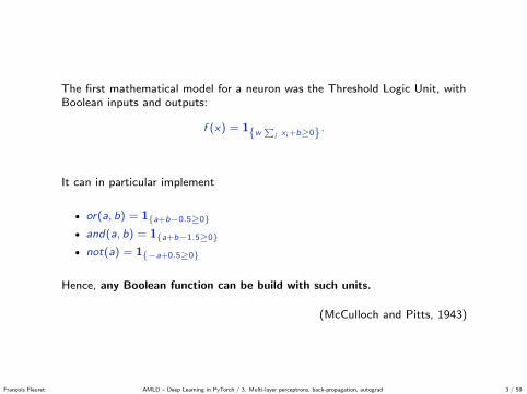
The first mathematical model for a neuron was the Threshold Logic Unit, withBoolean inputs and outputs:
f (x) = 1{w ∑i xi+b≥0}.
It can in particular implement
• or(a, b) = 1{a+b−0.5≥0}• and(a, b) = 1{a+b−1.5≥0}• not(a) = 1{−a+0.5≥0}
Hence, any Boolean function can be build with such units.
(McCulloch and Pitts, 1943)
Francois Fleuret AMLD – Deep Learning in PyTorch / 3. Multi-layer perceptrons, back-propagation, autograd 3 / 59

The perceptron is very similar
f (x) =
1 if∑i
wi xi + b ≥ 0
0 otherwise
but the inputs are real values and the weights can be different.
This model was originally motivated by biology, with wi being the synapticweights, and xi and f firing rates.
It is a (very) crude biological model.
(Rosenblatt, 1957)
Francois Fleuret AMLD – Deep Learning in PyTorch / 3. Multi-layer perceptrons, back-propagation, autograd 4 / 59

We can represent this as
x ·
w
+
b
σ y
Francois Fleuret AMLD – Deep Learning in PyTorch / 3. Multi-layer perceptrons, back-propagation, autograd 5 / 59

Given a training set
(xn, yn) ∈ RD × {−1, 1}, n = 1, . . . ,N,
a very simple scheme to train such a linear operator for classification is theperceptron algorithm:
1. Start with w0 = 0,
2. while ∃nk s.t. ynk(wk · xnk
)≤ 0, update wk+1 = wk + ynk xnk .
The bias b can be introduced as one of the ws by adding a constant componentto x equal to 1.
(Rosenblatt, 1957)
Francois Fleuret AMLD – Deep Learning in PyTorch / 3. Multi-layer perceptrons, back-propagation, autograd 6 / 59

def train_perceptron(x, y, nb_epochs_max):
w = Tensor(x.size (1)).zero_()
for e in range(nb_epochs_max):
nb_changes = 0
for i in range(x.size (0)):
if x[i].dot(w) * y[i] <= 0:
w = w + y[i] * x[i]
nb_changes = nb_changes + 1
if nb_changes == 0: break;
return w
Francois Fleuret AMLD – Deep Learning in PyTorch / 3. Multi-layer perceptrons, back-propagation, autograd 7 / 59

Francois Fleuret AMLD – Deep Learning in PyTorch / 3. Multi-layer perceptrons, back-propagation, autograd 8 / 59

Francois Fleuret AMLD – Deep Learning in PyTorch / 3. Multi-layer perceptrons, back-propagation, autograd 8 / 59

Francois Fleuret AMLD – Deep Learning in PyTorch / 3. Multi-layer perceptrons, back-propagation, autograd 8 / 59

Francois Fleuret AMLD – Deep Learning in PyTorch / 3. Multi-layer perceptrons, back-propagation, autograd 8 / 59

Francois Fleuret AMLD – Deep Learning in PyTorch / 3. Multi-layer perceptrons, back-propagation, autograd 8 / 59

Francois Fleuret AMLD – Deep Learning in PyTorch / 3. Multi-layer perceptrons, back-propagation, autograd 8 / 59

Francois Fleuret AMLD – Deep Learning in PyTorch / 3. Multi-layer perceptrons, back-propagation, autograd 8 / 59

Francois Fleuret AMLD – Deep Learning in PyTorch / 3. Multi-layer perceptrons, back-propagation, autograd 8 / 59

This crude algorithm works often surprisingly well. With MNIST’s “0”s asnegative class, and “1”s as positive one.
epoch 0 nb_changes 64 train_error 0.23%% test_error 0.19%%
epoch 1 nb_changes 24 train_error 0.07%% test_error 0.00%%
epoch 2 nb_changes 10 train_error 0.06%% test_error 0.05%%
epoch 3 nb_changes 6 train_error 0.03%% test_error 0.14%%
epoch 4 nb_changes 5 train_error 0.03%% test_error 0.09%%
epoch 5 nb_changes 4 train_error 0.02%% test_error 0.14%%
epoch 6 nb_changes 3 train_error 0.01%% test_error 0.14%%
epoch 7 nb_changes 2 train_error 0.00%% test_error 0.14%%
epoch 8 nb_changes 0 train_error 0.00%% test_error 0.14%%
Francois Fleuret AMLD – Deep Learning in PyTorch / 3. Multi-layer perceptrons, back-propagation, autograd 9 / 59

Limitation of linear classifiers
Francois Fleuret AMLD – Deep Learning in PyTorch / 3. Multi-layer perceptrons, back-propagation, autograd 10 / 59

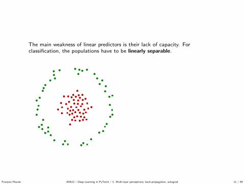
The main weakness of linear predictors is their lack of capacity. Forclassification, the populations have to be linearly separable.
“xor”
Francois Fleuret AMLD – Deep Learning in PyTorch / 3. Multi-layer perceptrons, back-propagation, autograd 11 / 59
The main weakness of linear predictors is their lack of capacity. Forclassification, the populations have to be linearly separable.
“xor”
Francois Fleuret AMLD – Deep Learning in PyTorch / 3. Multi-layer perceptrons, back-propagation, autograd 11 / 59

The main weakness of linear predictors is their lack of capacity. Forclassification, the populations have to be linearly separable.
“xor”
Francois Fleuret AMLD – Deep Learning in PyTorch / 3. Multi-layer perceptrons, back-propagation, autograd 11 / 59

The xor example can be solved by pre-processing the data to make the twopopulations linearly separable:
Φ : (xu , xv ) 7→ (xu , xv , xuxv ).
So we can model the xor with
f (x) = σ(w Φ(x) + b).
Francois Fleuret AMLD – Deep Learning in PyTorch / 3. Multi-layer perceptrons, back-propagation, autograd 12 / 59

We can apply the same to a more realistic binary classification problem:MNIST’s “8” vs. the other classes with a perceptron.
The original 28× 28 features are supplemented with the products of pairs offeatures taken at random.
0
1
2
3
4
5
6
7
103 104
Erro
r (%
)
Nb. of features
Train errorTest error
Francois Fleuret AMLD – Deep Learning in PyTorch / 3. Multi-layer perceptrons, back-propagation, autograd 13 / 59

Beside increasing capacity to reduce the bias, “feature design” may also be away of reducing capacity without hurting the bias, or with improving it.
In particular, good features should be invariant to perturbations of the signalknown to keep the value to predict unchanged.
Francois Fleuret AMLD – Deep Learning in PyTorch / 3. Multi-layer perceptrons, back-propagation, autograd 14 / 59

A classical example is the “Histogram of Oriented Gradient” descriptors (HOG),initially designed for person detection.
Roughly: divide the image in 8× 8 blocks, compute in each the distribution ofedge orientations over 9 bins.
Dalal and Triggs (2005) combined them with a linear predictor, and Dollar et al.(2009) extended them with other modalities into the “channel features”.
Francois Fleuret AMLD – Deep Learning in PyTorch / 3. Multi-layer perceptrons, back-propagation, autograd 15 / 59

Training a model composed of manually engineered features and a parametricmodel is now referred to as “shallow learning”.
The signal goes through a single processing trained from data.
A core notion of “Deep Learning” is precisely to avoid this dichotomy and torely on [“deep”] sequences of processing with limited hand-designed structures.
Francois Fleuret AMLD – Deep Learning in PyTorch / 3. Multi-layer perceptrons, back-propagation, autograd 16 / 59

Multi-Layer Perceptron
Francois Fleuret AMLD – Deep Learning in PyTorch / 3. Multi-layer perceptrons, back-propagation, autograd 17 / 59

We can combine several “layers”. With x(0) = x ,
∀l = 1, . . . , L, x(l) = σ(w (l)x(l−1) + b(l)
)and f (x ;w , b) = x(L).
x ×
w (1)
+
b(1)
σ . . . ×
w (L)
+
b(L)
σ y
Such a model is a Multi-Layer Perceptron (MLP).
B If σ is affine, this is an affine mapping.
Francois Fleuret AMLD – Deep Learning in PyTorch / 3. Multi-layer perceptrons, back-propagation, autograd 18 / 59

The two classical activation functions are the hyperbolic tangent
x 7→2
1 + e−2x− 1
−1
1
and the rectified linear unit (ReLU)
x 7→ max(0, x)
0
Francois Fleuret AMLD – Deep Learning in PyTorch / 3. Multi-layer perceptrons, back-propagation, autograd 19 / 59

The two classical activation functions are the hyperbolic tangent
x 7→2
1 + e−2x− 1
−1
1
and the rectified linear unit (ReLU)
x 7→ max(0, x)
0
Francois Fleuret AMLD – Deep Learning in PyTorch / 3. Multi-layer perceptrons, back-propagation, autograd 19 / 59

Under mild assumption on σ, we can approximate any continuous function
f : [0, 1]D → R
with a one hidden layer perceptron if it has enough units. This is the universalapproximation theorem.
B This says nothing about the number of units and the resulting mapping“complexity”.
Francois Fleuret AMLD – Deep Learning in PyTorch / 3. Multi-layer perceptrons, back-propagation, autograd 20 / 59

Training and gradient descent
Francois Fleuret AMLD – Deep Learning in PyTorch / 3. Multi-layer perceptrons, back-propagation, autograd 21 / 59

We saw that training consists of finding the model parameters minimizing anempirical risk or loss, for instance the mean-squared error (MSE)
L(w , b) =1
N
∑n
l (f (xn;w , b)− yn)2 .
Other losses are more fitting for classification, certain regression problems, ordensity estimation. We will come back to this.
In what we saw, we minimized the MSE with an analytic solution and theempirical error rate with the perceptron.
The general optimization method when dealing with an arbitrary loss and modelis the gradient descent.
Francois Fleuret AMLD – Deep Learning in PyTorch / 3. Multi-layer perceptrons, back-propagation, autograd 22 / 59

Given a functional
f : RD → Rx 7→ f (x1, . . . , xD),
its gradient is the mapping
∇f : RD → RD
x 7→(∂f
∂x1(x), . . . ,
∂f
∂xD(x)
).
Francois Fleuret AMLD – Deep Learning in PyTorch / 3. Multi-layer perceptrons, back-propagation, autograd 23 / 59

To minimize a functionalL : RD → R
the gradient descent uses local linear information to iteratively move toward a(local) minimum.
For w0 ∈ RD , consider an approximation of L around w0
Lw0 (w) = L(w0) +∇L(w0)T (w − w0) +1
2η‖w − w0‖2.
Note that the chosen quadratic term does not depend on L.
We have
∇Lw0 (w) = ∇L(w0) +1
η(w − w0),
which leads toargmin
wLw0 (w) = w0 − η∇L(w0).
Francois Fleuret AMLD – Deep Learning in PyTorch / 3. Multi-layer perceptrons, back-propagation, autograd 24 / 59

The resulting iterative rule takes the form of:
wt+1 = wt − η∇L(wt).
Which corresponds intuitively to “following the steepest descent”.
This finds a local minimum, and the choices of w0 and η are important.
Francois Fleuret AMLD – Deep Learning in PyTorch / 3. Multi-layer perceptrons, back-propagation, autograd 25 / 59

η = 0.125
w0
LL
Francois Fleuret AMLD – Deep Learning in PyTorch / 3. Multi-layer perceptrons, back-propagation, autograd 26 / 59

η = 0.125
w1
LL
Francois Fleuret AMLD – Deep Learning in PyTorch / 3. Multi-layer perceptrons, back-propagation, autograd 26 / 59

η = 0.125
w2
LL
Francois Fleuret AMLD – Deep Learning in PyTorch / 3. Multi-layer perceptrons, back-propagation, autograd 26 / 59

η = 0.125
w3
LL
Francois Fleuret AMLD – Deep Learning in PyTorch / 3. Multi-layer perceptrons, back-propagation, autograd 26 / 59

η = 0.125
w4
LL
Francois Fleuret AMLD – Deep Learning in PyTorch / 3. Multi-layer perceptrons, back-propagation, autograd 26 / 59

η = 0.125
w5
LL
Francois Fleuret AMLD – Deep Learning in PyTorch / 3. Multi-layer perceptrons, back-propagation, autograd 26 / 59

η = 0.125
w6
LL
Francois Fleuret AMLD – Deep Learning in PyTorch / 3. Multi-layer perceptrons, back-propagation, autograd 26 / 59

η = 0.125
w7
LL
Francois Fleuret AMLD – Deep Learning in PyTorch / 3. Multi-layer perceptrons, back-propagation, autograd 26 / 59

η = 0.125
w8
LL
Francois Fleuret AMLD – Deep Learning in PyTorch / 3. Multi-layer perceptrons, back-propagation, autograd 26 / 59

η = 0.125
w9
LL
Francois Fleuret AMLD – Deep Learning in PyTorch / 3. Multi-layer perceptrons, back-propagation, autograd 26 / 59

η = 0.125
w10
LL
Francois Fleuret AMLD – Deep Learning in PyTorch / 3. Multi-layer perceptrons, back-propagation, autograd 26 / 59

η = 0.125
w11
LL
Francois Fleuret AMLD – Deep Learning in PyTorch / 3. Multi-layer perceptrons, back-propagation, autograd 26 / 59

η = 0.125
w0
LL
Francois Fleuret AMLD – Deep Learning in PyTorch / 3. Multi-layer perceptrons, back-propagation, autograd 27 / 59

η = 0.125
w1
LL
Francois Fleuret AMLD – Deep Learning in PyTorch / 3. Multi-layer perceptrons, back-propagation, autograd 27 / 59

η = 0.125
w2
LL
Francois Fleuret AMLD – Deep Learning in PyTorch / 3. Multi-layer perceptrons, back-propagation, autograd 27 / 59

η = 0.125
w3
LL
Francois Fleuret AMLD – Deep Learning in PyTorch / 3. Multi-layer perceptrons, back-propagation, autograd 27 / 59

η = 0.125
w4
LL
Francois Fleuret AMLD – Deep Learning in PyTorch / 3. Multi-layer perceptrons, back-propagation, autograd 27 / 59

η = 0.125
w5
LL
Francois Fleuret AMLD – Deep Learning in PyTorch / 3. Multi-layer perceptrons, back-propagation, autograd 27 / 59

η = 0.125
w6
LL
Francois Fleuret AMLD – Deep Learning in PyTorch / 3. Multi-layer perceptrons, back-propagation, autograd 27 / 59

η = 0.125
w7
LL
Francois Fleuret AMLD – Deep Learning in PyTorch / 3. Multi-layer perceptrons, back-propagation, autograd 27 / 59

η = 0.125
w8
LL
Francois Fleuret AMLD – Deep Learning in PyTorch / 3. Multi-layer perceptrons, back-propagation, autograd 27 / 59

η = 0.125
w9
LL
Francois Fleuret AMLD – Deep Learning in PyTorch / 3. Multi-layer perceptrons, back-propagation, autograd 27 / 59

η = 0.125
w10
LL
Francois Fleuret AMLD – Deep Learning in PyTorch / 3. Multi-layer perceptrons, back-propagation, autograd 27 / 59

η = 0.125
w11
LL
Francois Fleuret AMLD – Deep Learning in PyTorch / 3. Multi-layer perceptrons, back-propagation, autograd 27 / 59

η = 0.5
w0
LL
Francois Fleuret AMLD – Deep Learning in PyTorch / 3. Multi-layer perceptrons, back-propagation, autograd 28 / 59

η = 0.5
w1
LL
Francois Fleuret AMLD – Deep Learning in PyTorch / 3. Multi-layer perceptrons, back-propagation, autograd 28 / 59

η = 0.5
w2
LL
Francois Fleuret AMLD – Deep Learning in PyTorch / 3. Multi-layer perceptrons, back-propagation, autograd 28 / 59

η = 0.5
w3
LL
Francois Fleuret AMLD – Deep Learning in PyTorch / 3. Multi-layer perceptrons, back-propagation, autograd 28 / 59

η = 0.5
w4
LL
Francois Fleuret AMLD – Deep Learning in PyTorch / 3. Multi-layer perceptrons, back-propagation, autograd 28 / 59

η = 0.5
w5
LL
Francois Fleuret AMLD – Deep Learning in PyTorch / 3. Multi-layer perceptrons, back-propagation, autograd 28 / 59

η = 0.5
w6
LL
Francois Fleuret AMLD – Deep Learning in PyTorch / 3. Multi-layer perceptrons, back-propagation, autograd 28 / 59

η = 0.5
w7
LL
Francois Fleuret AMLD – Deep Learning in PyTorch / 3. Multi-layer perceptrons, back-propagation, autograd 28 / 59

η = 0.5
w8
LL
Francois Fleuret AMLD – Deep Learning in PyTorch / 3. Multi-layer perceptrons, back-propagation, autograd 28 / 59

η = 0.5
w9
LL
Francois Fleuret AMLD – Deep Learning in PyTorch / 3. Multi-layer perceptrons, back-propagation, autograd 28 / 59

η = 0.5
w10
LL
Francois Fleuret AMLD – Deep Learning in PyTorch / 3. Multi-layer perceptrons, back-propagation, autograd 28 / 59

η = 0.5
w11
LL
Francois Fleuret AMLD – Deep Learning in PyTorch / 3. Multi-layer perceptrons, back-propagation, autograd 28 / 59

0 0.2
0.4 0.6
0.8 1 0
0.2 0.4
0.6 0.8
1
0.6
0.8
1
1.2
1.4
Francois Fleuret AMLD – Deep Learning in PyTorch / 3. Multi-layer perceptrons, back-propagation, autograd 29 / 59

0
0.2
0.4
0.6
0.8
1
0 0.2 0.4 0.6 0.8 1
Francois Fleuret AMLD – Deep Learning in PyTorch / 3. Multi-layer perceptrons, back-propagation, autograd 29 / 59

0
0.2
0.4
0.6
0.8
1
0 0.2 0.4 0.6 0.8 1
Francois Fleuret AMLD – Deep Learning in PyTorch / 3. Multi-layer perceptrons, back-propagation, autograd 29 / 59

0
0.2
0.4
0.6
0.8
1
0 0.2 0.4 0.6 0.8 1
Francois Fleuret AMLD – Deep Learning in PyTorch / 3. Multi-layer perceptrons, back-propagation, autograd 29 / 59

from torch import nn
from torch.autograd import Variable
from torchvision import datasets
nb_samples , positive_class = 1000, 5
data = datasets.MNIST(’./data/mnist/’, train = True , download = True)
x = data.train_data.narrow(0, 0, nb_samples).view(-1, 28 * 28).float ()
y = (data.train_labels.narrow(0, 0, nb_samples) == positive_class).float()
x.sub_(x.mean()).div_(x.std()) # Normalize the data
x, y = Variable(x), Variable(y) # Some dark magic
model = nn.Sequential(nn.Linear (784, 200), nn.ReLU(), nn.Linear (200, 1))
for k in range (1000):
yhat = model(x).view(-1) # Makes the vector 1d
loss = (yhat - y).pow(2).mean()
if k%100 == 0:
nb_errors = ((yhat.data > 0.5).float() != y.data).sum()
print(k, loss.data[0], nb_errors)
model.zero_grad ()
loss.backward () # Automagically compute the gradient
for p in model.parameters (): p.data.sub_(1e-2 * p.grad.data)
Francois Fleuret AMLD – Deep Learning in PyTorch / 3. Multi-layer perceptrons, back-propagation, autograd 30 / 59

0 0.19517871737480164 92
100 0.0376046821475029 38
200 0.025428157299757004 19
300 0.019106458872556686 13
400 0.015085148625075817 8
500 0.012246628291904926 4
600 0.01010703295469284 2
700 0.008458797819912434 2
800 0.007151678670197725 1
900 0.006096927914768457 0
Note that these are the training loss and error.
Francois Fleuret AMLD – Deep Learning in PyTorch / 3. Multi-layer perceptrons, back-propagation, autograd 31 / 59

Back-propagation
Francois Fleuret AMLD – Deep Learning in PyTorch / 3. Multi-layer perceptrons, back-propagation, autograd 32 / 59

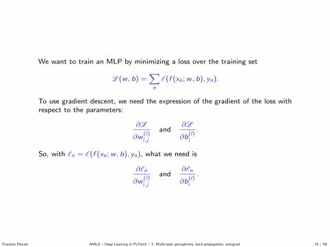
We want to train an MLP by minimizing a loss over the training set
L(w , b) =∑n
l(f (xn;w , b), yn).
To use gradient descent, we need the expression of the gradient of the loss withrespect to the parameters:
∂L
∂w(l)i,j
and∂L
∂b(l)i
.
So, with ln = l(f (xn;w , b), yn), what we need is
∂ln
∂w(l)i,j
and∂ln
∂b(l)i
.
Francois Fleuret AMLD – Deep Learning in PyTorch / 3. Multi-layer perceptrons, back-propagation, autograd 33 / 59

The core principle of the back-propagation algorithm is the “chain rule” fromdifferential calculus:
(g ◦ f )′ = (g ′ ◦ f )f ′
which generalizes to longer compositions and higher dimensions
JfN◦fN−1◦···◦f1 (x) =N∏
n=1
Jfn (fn−1 ◦ · · · ◦ f1(x)),
where Jf (x) is the Jacobian of f at x , that is the matrix of the linearapproximation of f in the neighborhood of x .
The linear approximation of a composition of mappings is the product of theirindividual linear approximations.
What follows is exactly this principle applied to a MLP.
Francois Fleuret AMLD – Deep Learning in PyTorch / 3. Multi-layer perceptrons, back-propagation, autograd 34 / 59

x(l−1) ×
w (l)
+
b(l)
s(l) σ x(l)
[∂l
∂x(l)
][∂l
∂s(l)
]� σ′·T×
[∂l
∂x(l−1)
]
[∂l
∂b(l)
][[∂l
∂w (l)
]]
× ·T
Francois Fleuret AMLD – Deep Learning in PyTorch / 3. Multi-layer perceptrons, back-propagation, autograd 35 / 59

x(l−1) ×
w (l)
+
b(l)
s(l) σ x(l)
[∂l
∂x(l)
][∂l
∂s(l)
]� σ′·T×
[∂l
∂x(l−1)
]
[∂l
∂b(l)
][[∂l
∂w (l)
]]
× ·T
Francois Fleuret AMLD – Deep Learning in PyTorch / 3. Multi-layer perceptrons, back-propagation, autograd 35 / 59

x(l−1) ×
w (l)
+
b(l)
s(l) σ x(l)
[∂l
∂x(l)
]
[∂l
∂s(l)
]� σ′·T×
[∂l
∂x(l−1)
]
[∂l
∂b(l)
][[∂l
∂w (l)
]]
× ·T
Francois Fleuret AMLD – Deep Learning in PyTorch / 3. Multi-layer perceptrons, back-propagation, autograd 35 / 59

x(l−1) ×
w (l)
+
b(l)
s(l) σ x(l)
[∂l
∂x(l)
][∂l
∂s(l)
]� σ′
·T×[
∂l
∂x(l−1)
]
[∂l
∂b(l)
][[∂l
∂w (l)
]]
× ·T
∂l
∂s(l)i
=∂l
∂x(l)i
σ′(s
(l)i
)
Francois Fleuret AMLD – Deep Learning in PyTorch / 3. Multi-layer perceptrons, back-propagation, autograd 35 / 59

x(l−1) ×
w (l)
+
b(l)
s(l) σ x(l)
[∂l
∂x(l)
][∂l
∂s(l)
]� σ′·T×
[∂l
∂x(l−1)
]
[∂l
∂b(l)
][[∂l
∂w (l)
]]
× ·T
∂l
∂x(l−1)j
=∑i
w(l)i,j
∂l
∂s(l)i
Francois Fleuret AMLD – Deep Learning in PyTorch / 3. Multi-layer perceptrons, back-propagation, autograd 35 / 59

x(l−1) ×
w (l)
+
b(l)
s(l) σ x(l)
[∂l
∂x(l)
][∂l
∂s(l)
]� σ′·T×
[∂l
∂x(l−1)
]
[∂l
∂b(l)
]
[[∂l
∂w (l)
]]
× ·T
∂l
∂b(l)i
=∂l
∂s(l)i
Francois Fleuret AMLD – Deep Learning in PyTorch / 3. Multi-layer perceptrons, back-propagation, autograd 35 / 59

x(l−1) ×
w (l)
+
b(l)
s(l) σ x(l)
[∂l
∂x(l)
][∂l
∂s(l)
]� σ′·T×
[∂l
∂x(l−1)
]
[∂l
∂b(l)
][[∂l
∂w (l)
]]
× ·T
∂l
∂w(l)i,j
=∂l
∂s(l)i
x(l−1)j
Francois Fleuret AMLD – Deep Learning in PyTorch / 3. Multi-layer perceptrons, back-propagation, autograd 35 / 59

x(l−1) ×
w (l)
+
b(l)
s(l) σ x(l)
[∂l
∂x(l)
][∂l
∂s(l)
]� σ′·T×
[∂l
∂x(l−1)
]
[∂l
∂b(l)
][[∂l
∂w (l)
]]
× ·T
Francois Fleuret AMLD – Deep Learning in PyTorch / 3. Multi-layer perceptrons, back-propagation, autograd 35 / 59

Forward pass
∀n, x(0)n = xn, ∀l = 1, . . . , L,
{s
(l)n = w (l)x
(l−1)n + b(l)
x(l)n = σ
(s
(l)n
)
Backward pass
[∂ln
∂x(L)n
]= ∇1ln
(x
(L)n
)if l < L,
[∂ln
∂x(l)n
]=(w l+1
)T [ ∂ln
∂s l+1
] [∂ln
∂s(l)
]=
[∂ln
∂x(l)n
]� σ′
(s(l))
[[∂ln
∂w (l)
]]=
[∂ln
∂s(l)
](x
(l−1)n
)T [∂ln
∂b(l)
]=
[∂ln
∂s(l)
].
Gradient step
w (l) ← w (l) − η∑n
[[∂ln
∂w (l)
]]b(l) ← b(l) − η
∑n
[∂ln
∂b(l)
]
Francois Fleuret AMLD – Deep Learning in PyTorch / 3. Multi-layer perceptrons, back-propagation, autograd 36 / 59

Forward pass
∀n, x(0)n = xn, ∀l = 1, . . . , L,
{s
(l)n = w (l)x
(l−1)n + b(l)
x(l)n = σ
(s
(l)n
)Backward pass
[∂ln
∂x(L)n
]= ∇1ln
(x
(L)n
)if l < L,
[∂ln
∂x(l)n
]=(w l+1
)T [ ∂ln
∂s l+1
] [∂ln
∂s(l)
]=
[∂ln
∂x(l)n
]� σ′
(s(l))
[[∂ln
∂w (l)
]]=
[∂ln
∂s(l)
](x
(l−1)n
)T [∂ln
∂b(l)
]=
[∂ln
∂s(l)
].
Gradient step
w (l) ← w (l) − η∑n
[[∂ln
∂w (l)
]]b(l) ← b(l) − η
∑n
[∂ln
∂b(l)
]
Francois Fleuret AMLD – Deep Learning in PyTorch / 3. Multi-layer perceptrons, back-propagation, autograd 36 / 59

In spite of its hairy formalization, the backward pass is conceptually trivial:Apply the chain rule again and again.
As for the forward pass, it can be expressed in tensorial form. Heavycomputation is concentrated in linear operations, and all the non-linearities gointo component-wise operations.
Regarding computation, the rule of thumb is that the backward pass is twicemore expensive than the forward one.
Francois Fleuret AMLD – Deep Learning in PyTorch / 3. Multi-layer perceptrons, back-propagation, autograd 37 / 59

DAG networks
Francois Fleuret AMLD – Deep Learning in PyTorch / 3. Multi-layer perceptrons, back-propagation, autograd 38 / 59

Everything we have seen for an MLP
x ×
w (1)
+
b(1)
σ ×
w (2)
+
b(2)
σ f (x)
can be generalized to an arbitrary “Directed Acyclic Graph” (DAG) of operators
x
φ(1)
φ(2)
f (x)φ(3)
w (1)
w (2)
Francois Fleuret AMLD – Deep Learning in PyTorch / 3. Multi-layer perceptrons, back-propagation, autograd 39 / 59

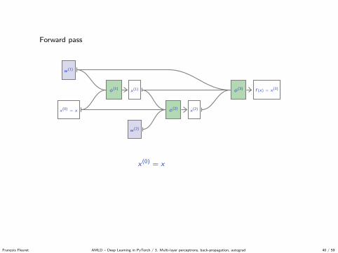
Forward pass
x(0) = x
x(1)φ(1)
x(2)φ(2)
f (x) = x(3)φ(3)
w (1)
w (2)
x(0) = x
x(1) = φ(1)(x(0);w (1))
x(2) = φ(2)(x(0), x(1);w (2))
f (x) = x(3) = φ(3)(x(1), x(2);w (1))
Francois Fleuret AMLD – Deep Learning in PyTorch / 3. Multi-layer perceptrons, back-propagation, autograd 40 / 59
Forward pass
x(0) = x
x(1)φ(1)
x(2)φ(2)
f (x) = x(3)φ(3)
w (1)
w (2)
x(0) = x
x(1) = φ(1)(x(0);w (1))
x(2) = φ(2)(x(0), x(1);w (2))
f (x) = x(3) = φ(3)(x(1), x(2);w (1))
Francois Fleuret AMLD – Deep Learning in PyTorch / 3. Multi-layer perceptrons, back-propagation, autograd 40 / 59

Forward pass
x(0) = x
x(1)φ(1)
x(2)φ(2)
f (x) = x(3)φ(3)
w (1)
w (2)
x(0) = x
x(1) = φ(1)(x(0);w (1))
x(2) = φ(2)(x(0), x(1);w (2))
f (x) = x(3) = φ(3)(x(1), x(2);w (1))
Francois Fleuret AMLD – Deep Learning in PyTorch / 3. Multi-layer perceptrons, back-propagation, autograd 40 / 59

Forward pass
x(0) = x
x(1)φ(1)
x(2)φ(2)
f (x) = x(3)φ(3)
w (1)
w (2)
x(0) = x
x(1) = φ(1)(x(0);w (1))
x(2) = φ(2)(x(0), x(1);w (2))
f (x) = x(3) = φ(3)(x(1), x(2);w (1))
Francois Fleuret AMLD – Deep Learning in PyTorch / 3. Multi-layer perceptrons, back-propagation, autograd 40 / 59

Forward pass
x(0) = x
x(1)φ(1)
x(2)φ(2)
f (x) = x(3)φ(3)
w (1)
w (2)
x(0) = x
x(1) = φ(1)(x(0);w (1))
x(2) = φ(2)(x(0), x(1);w (2))
f (x) = x(3) = φ(3)(x(1), x(2);w (1))
Francois Fleuret AMLD – Deep Learning in PyTorch / 3. Multi-layer perceptrons, back-propagation, autograd 40 / 59

Backward pass, derivatives w.r.t activations
x(0) = x
x(1)φ(1)
x(2)φ(2)
f (x) = x(3)φ(3)
w (1)
w (2)
[∂l
∂x(2)
]=
[∂x(3)
∂x(2)
][∂l
∂x(3)
]= Jφ(3)|x (2)
[∂l
∂x(3)
][∂l
∂x(1)
]=
[∂x(2)
∂x(1)
][∂l
∂x(2)
]+
[∂x(3)
∂x(1)
] [∂l
∂x(3)
]= Jφ(2)|x (1)
[∂l
∂x(2)
]+ Jφ(3)|x (1)
[∂l
∂x(3)
][∂l
∂x(0)
]=
[∂x(1)
∂x(0)
][∂l
∂x(1)
]+
[∂x(2)
∂x(0)
] [∂l
∂x(2)
]= Jφ(1)|x (0)
[∂l
∂x(1)
]+ Jφ(2)|x (0)
[∂l
∂x(2)
]
Francois Fleuret AMLD – Deep Learning in PyTorch / 3. Multi-layer perceptrons, back-propagation, autograd 41 / 59

Backward pass, derivatives w.r.t activations
x(0) = x
x(1)φ(1)
x(2)φ(2)
f (x) = x(3)φ(3)
w (1)
w (2)
[∂l
∂x(2)
]=
[∂x(3)
∂x(2)
][∂l
∂x(3)
]= Jφ(3)|x (2)
[∂l
∂x(3)
]
[∂l
∂x(1)
]=
[∂x(2)
∂x(1)
][∂l
∂x(2)
]+
[∂x(3)
∂x(1)
] [∂l
∂x(3)
]= Jφ(2)|x (1)
[∂l
∂x(2)
]+ Jφ(3)|x (1)
[∂l
∂x(3)
][∂l
∂x(0)
]=
[∂x(1)
∂x(0)
][∂l
∂x(1)
]+
[∂x(2)
∂x(0)
] [∂l
∂x(2)
]= Jφ(1)|x (0)
[∂l
∂x(1)
]+ Jφ(2)|x (0)
[∂l
∂x(2)
]
Francois Fleuret AMLD – Deep Learning in PyTorch / 3. Multi-layer perceptrons, back-propagation, autograd 41 / 59

Backward pass, derivatives w.r.t activations
x(0) = x
x(1)φ(1)
x(2)φ(2)
f (x) = x(3)φ(3)
w (1)
w (2)
[∂l
∂x(2)
]=
[∂x(3)
∂x(2)
][∂l
∂x(3)
]= Jφ(3)|x (2)
[∂l
∂x(3)
][∂l
∂x(1)
]=
[∂x(2)
∂x(1)
][∂l
∂x(2)
]+
[∂x(3)
∂x(1)
] [∂l
∂x(3)
]= Jφ(2)|x (1)
[∂l
∂x(2)
]+ Jφ(3)|x (1)
[∂l
∂x(3)
]
[∂l
∂x(0)
]=
[∂x(1)
∂x(0)
][∂l
∂x(1)
]+
[∂x(2)
∂x(0)
] [∂l
∂x(2)
]= Jφ(1)|x (0)
[∂l
∂x(1)
]+ Jφ(2)|x (0)
[∂l
∂x(2)
]
Francois Fleuret AMLD – Deep Learning in PyTorch / 3. Multi-layer perceptrons, back-propagation, autograd 41 / 59

Backward pass, derivatives w.r.t activations
x(0) = x
x(1)φ(1)
x(2)φ(2)
f (x) = x(3)φ(3)
w (1)
w (2)
[∂l
∂x(2)
]=
[∂x(3)
∂x(2)
][∂l
∂x(3)
]= Jφ(3)|x (2)
[∂l
∂x(3)
][∂l
∂x(1)
]=
[∂x(2)
∂x(1)
][∂l
∂x(2)
]+
[∂x(3)
∂x(1)
] [∂l
∂x(3)
]= Jφ(2)|x (1)
[∂l
∂x(2)
]+ Jφ(3)|x (1)
[∂l
∂x(3)
][∂l
∂x(0)
]=
[∂x(1)
∂x(0)
][∂l
∂x(1)
]+
[∂x(2)
∂x(0)
] [∂l
∂x(2)
]= Jφ(1)|x (0)
[∂l
∂x(1)
]+ Jφ(2)|x (0)
[∂l
∂x(2)
]
Francois Fleuret AMLD – Deep Learning in PyTorch / 3. Multi-layer perceptrons, back-propagation, autograd 41 / 59

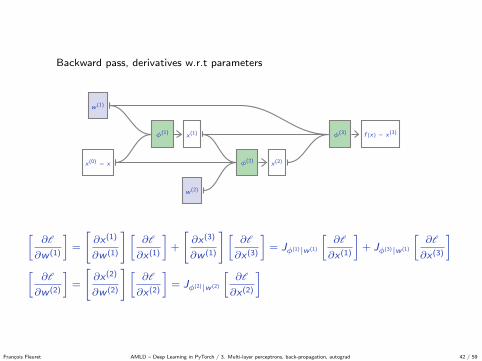
Backward pass, derivatives w.r.t parameters
x(0) = x
x(1)φ(1)
x(2)φ(2)
f (x) = x(3)φ(3)
w (1)
w (2)
[∂l
∂w (1)
]=
[∂x(1)
∂w (1)
] [∂l
∂x(1)
]+
[∂x(3)
∂w (1)
][∂l
∂x(3)
]= Jφ(1)|w (1)
[∂l
∂x(1)
]+ Jφ(3)|w (1)
[∂l
∂x(3)
][∂l
∂w (2)
]=
[∂x(2)
∂w (2)
] [∂l
∂x(2)
]= Jφ(2)|w (2)
[∂l
∂x(2)
]
Francois Fleuret AMLD – Deep Learning in PyTorch / 3. Multi-layer perceptrons, back-propagation, autograd 42 / 59

Backward pass, derivatives w.r.t parameters
x(0) = x
x(1)φ(1)
x(2)φ(2)
f (x) = x(3)φ(3)
w (1)
w (2)
[∂l
∂w (1)
]=
[∂x(1)
∂w (1)
] [∂l
∂x(1)
]+
[∂x(3)
∂w (1)
][∂l
∂x(3)
]= Jφ(1)|w (1)
[∂l
∂x(1)
]+ Jφ(3)|w (1)
[∂l
∂x(3)
]
[∂l
∂w (2)
]=
[∂x(2)
∂w (2)
] [∂l
∂x(2)
]= Jφ(2)|w (2)
[∂l
∂x(2)
]
Francois Fleuret AMLD – Deep Learning in PyTorch / 3. Multi-layer perceptrons, back-propagation, autograd 42 / 59
Backward pass, derivatives w.r.t parameters
x(0) = x
x(1)φ(1)
x(2)φ(2)
f (x) = x(3)φ(3)
w (1)
w (2)
[∂l
∂w (1)
]=
[∂x(1)
∂w (1)
] [∂l
∂x(1)
]+
[∂x(3)
∂w (1)
][∂l
∂x(3)
]= Jφ(1)|w (1)
[∂l
∂x(1)
]+ Jφ(3)|w (1)
[∂l
∂x(3)
][∂l
∂w (2)
]=
[∂x(2)
∂w (2)
] [∂l
∂x(2)
]= Jφ(2)|w (2)
[∂l
∂x(2)
]
Francois Fleuret AMLD – Deep Learning in PyTorch / 3. Multi-layer perceptrons, back-propagation, autograd 42 / 59

So if we have a library of “tensor operators”, and implementations of
(x1, . . . , xd ,w) 7→ φ(x1, . . . , xd ;w)
∀c, (x1, . . . , xd ,w) 7→ Jφ|xc (x1, . . . , xd ;w)
(x1, . . . , xd ,w) 7→ Jφ|w (x1, . . . , xd ;w),
we can build an arbitrary directed acyclic graph with these operators at thenodes, compute the response of the resulting mapping, and compute itsgradient with back-prop.
Francois Fleuret AMLD – Deep Learning in PyTorch / 3. Multi-layer perceptrons, back-propagation, autograd 43 / 59

Writing from scratch a large neural network is complex and error-prone.
Multiple frameworks provide libraries of tensor operators and mechanisms tocombine them into DAGs and automatically differentiate them.
Language(s) License Main backer
PyTorch Python BSD Facebook
Caffe2 C++, Python Apache Facebook
TensorFlow Python, C++ Apache Google
MXNet Python, C++, R, Scala Apache Amazon
CNTK Python, C++ MIT Microsoft
Torch Lua BSD Facebook
Theano Python BSD U. of Montreal
Caffe C++ BSD 2 clauses U. of CA, Berkeley
One approach is to define the nodes and edges of such a DAG statically (Torch,TensorFlow, Caffe, Theano, etc.)
Francois Fleuret AMLD – Deep Learning in PyTorch / 3. Multi-layer perceptrons, back-propagation, autograd 44 / 59
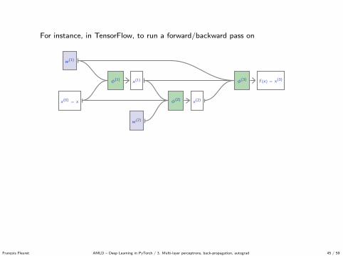
For instance, in TensorFlow, to run a forward/backward pass on
x(0) = x
x(1)φ(1)
x(2)φ(2)
f (x) = x(3)φ(3)
w (1)
w (2)
with
φ(1)(x(0);w (1)
)= w (1)x(0)
φ(2)(x(0), x(1);w (2)
)= x(0) + w (2)x(1)
φ(3)(x(1), x(2);w (1)
)= w (1)
(x(1) + x(2)
)
we can do
w1 = tf.Variable(tf.random_normal ([5, 5]))
w2 = tf.Variable(tf.random_normal ([5, 5]))
x = tf.Variable(tf.random_normal ([5, 1]))
x0 = x
x1 = tf.matmul(w1 , x0)
x2 = x0 + tf.matmul(w2, x1)
x3 = tf.matmul(w1 , x1 + x2)
q = tf.norm(x3)
gw1 , gw2 = tf.gradients(q, [w1, w2])
with tf.Session () as sess:
sess.run(tf.global_variables_initializer ())
_grads = sess.run(grads)
Francois Fleuret AMLD – Deep Learning in PyTorch / 3. Multi-layer perceptrons, back-propagation, autograd 45 / 59

Autograd
Francois Fleuret AMLD – Deep Learning in PyTorch / 3. Multi-layer perceptrons, back-propagation, autograd 46 / 59

The forward pass is “just” a computation as usual. The graph structure isneeded for the backward pass only.
The specification of the graph looks a lot like the forward pass, and theoperations of the forward pass fully define those of the backward.
PyTorch provides Variable s, which can be used as Tensor s, with theadvantage that during any computation, the graph of operations tocompute the gradient wrt any quantity is automatically constructed.
This “autograd” mechanism has two main benefits:
• Simpler syntax: one just need to write the forward pass as a standardcomputation,
• greater flexibility: Since the graph is not static, the forward pass can bedynamically modulated.
Francois Fleuret AMLD – Deep Learning in PyTorch / 3. Multi-layer perceptrons, back-propagation, autograd 47 / 59

To use autograd, use torch.autograd.Variable s instead of torch.Tensor s.
Most of the Tensor operations [have corresponding operations that] acceptVariable .
A Variable is a wrapper around a Tensor , with the following fields
• data is the Tensor containing the data itself,
• grad is a Variable of same dimension to sum the gradient,
• requires grad is a Boolean stating if we need the gradient w.r.t this
Variable (default is False ).
A Parameter is a Variable with requires grad to True by default, andknown to be a parameter by various utility functions.
Francois Fleuret AMLD – Deep Learning in PyTorch / 3. Multi-layer perceptrons, back-propagation, autograd 48 / 59

B A Variable can only embed a Tensor , so functions returning a scalar(e.g. a loss) now return a 1d Variable with a single value.
Francois Fleuret AMLD – Deep Learning in PyTorch / 3. Multi-layer perceptrons, back-propagation, autograd 49 / 59

torch.autograd.grad(outputs, inputs) computes and returns the sum of
gradients of outputs wrt the specified inputs. This is always a tuple .
An alternative is to use torch.autograd.backward(variables) or
Variable.backward() , which accumulates the gradients in the grad fields of
the leaf Variable s.
Francois Fleuret AMLD – Deep Learning in PyTorch / 3. Multi-layer perceptrons, back-propagation, autograd 50 / 59

Consider a simple example (x1, x2, x3) = (1, 2, 2), and
l = ‖x‖ =√
x21 + x2
2 + x23 .
We have l = 3 and∂l
∂xi=
xi
‖x‖.
>>> from torch import Tensor
>>> from torch.autograd import Variable
>>> x = Variable(Tensor ([1, 2, 2]), requires_grad = True)
>>> l = x.norm()
>>> l
Variable containing:
3
[torch.FloatTensor of size 1]
>>> l.backward ()
>>> x.grad
Variable containing:
0.3333
0.6667
0.6667
[torch.FloatTensor of size 3]
Francois Fleuret AMLD – Deep Learning in PyTorch / 3. Multi-layer perceptrons, back-propagation, autograd 51 / 59

For instance, in PyTorch, to run a forward/backward pass on
x(0) = x
x(1)φ(1)
x(2)φ(2)
f (x) = x(3)φ(3)
w (1)
w (2)
with
φ(1)(x(0);w (1)
)= w (1)x(0)
φ(2)(x(0), x(1);w (2)
)= x(0) + w (2)x(1)
φ(3)(x(1), x(2);w (1)
)= w (1)
(x(1) + x(2)
)
we can do
w1 = Parameter(Tensor(5, 5).normal_ ())
w2 = Parameter(Tensor(5, 5).normal_ ())
x = Variable(Tensor (5).normal_ ())
x0 = x
x1 = w1.mv(x0)
x2 = x0 + w2.mv(x1)
x3 = w1.mv(x1 + x2)
q = x3.norm()
q.backward ()
Francois Fleuret AMLD – Deep Learning in PyTorch / 3. Multi-layer perceptrons, back-propagation, autograd 52 / 59

We can look precisely at the graph built during a computation.
x = Parameter(Tensor ([1, 2, 2]))
q = x.norm()
q [1]
NormBackward0
AccumulateGrad
x [3]
This graph was generated with
https://fleuret.org/git/agtree2dot
and Graphviz.
Francois Fleuret AMLD – Deep Learning in PyTorch / 3. Multi-layer perceptrons, back-propagation, autograd 53 / 59

w1 = Parameter(Tensor (20, 10))
b1 = Parameter(Tensor (20))
w2 = Parameter(Tensor(5, 20))
b2 = Parameter(Tensor (5))
x = Variable(Tensor (10).normal_ ())
h = torch.tanh(w1.mv(x) + b1)
y = torch.tanh(w2.mv(h) + b2)
target = Variable(Tensor (5).normal_ ())
loss = (y - target).pow(2).sum()
loss [1]
SumBackward0
PowBackward0
SubBackward1
TanhBackward0
AddBackward1
0 1
MvBackward
0 1AccumulateGrad
AccumulateGrad TanhBackward0
w2 [5, 20]AddBackward1
0 1
MvBackward AccumulateGrad
AccumulateGrad
w1 [20, 10]
b1 [20]
b2 [5]
Francois Fleuret AMLD – Deep Learning in PyTorch / 3. Multi-layer perceptrons, back-propagation, autograd 54 / 59

w = Parameter(Tensor(3, 10, 10))
def blah(k, x):
for i in range(k):
x = torch.tanh(w[i].mv(x))
return x
u = blah(1, Variable(Tensor (10)))
v = blah(3, Variable(Tensor (10)))
q = u.dot(v)
Variable [1]
DotBackward
0 1
TanhBackward0 TanhBackward0
MvBackward
IndexBackward
AccumulateGrad
Parameter [3, 10, 10]
MvBackward
0 1
IndexBackward
TanhBackward0
MvBackward
0 1
IndexBackward
TanhBackward0
MvBackward
IndexBackward
Francois Fleuret AMLD – Deep Learning in PyTorch / 3. Multi-layer perceptrons, back-propagation, autograd 55 / 59

B Variable.backward() accumulates the gradients in the different
Variable s, so one may have to zero them before.
This accumulating behavior is desirable in particular to compute the gradient ofa loss summed over several “mini-batches,” or the gradient of a sum of losses.
BAlthough they are related, the autograd graph is not the network’sstructure, but the graph of operations to compute the gradient. It canbe data-dependent and miss or replicate sub-parts of the network.
Francois Fleuret AMLD – Deep Learning in PyTorch / 3. Multi-layer perceptrons, back-propagation, autograd 56 / 59

Weight sharing
Francois Fleuret AMLD – Deep Learning in PyTorch / 3. Multi-layer perceptrons, back-propagation, autograd 57 / 59

In our generalized DAG formulation, we have in particular implicitly allowed thesame parameters to modulate different parts of the processing.
For instance w (1) in our example parametrizes both φ(1) and φ(3).
x(0) = x
x(1)φ(1)
x(2)φ(2)
f (x) = x(3)φ(3)
w (1)
w (2)
This is called weight sharing.
Francois Fleuret AMLD – Deep Learning in PyTorch / 3. Multi-layer perceptrons, back-propagation, autograd 58 / 59

Weight sharing allows in particular to build siamese networks where a fullsub-network is replicated several times.
x(0) = x
ψu × + σ u(1) × + σ u(2)
ψv × + σ v (1) × + σ v (2)
φ x(1)w (1) b(1) w (2) b(2)
Francois Fleuret AMLD – Deep Learning in PyTorch / 3. Multi-layer perceptrons, back-propagation, autograd 59 / 59

The end
References
N. Dalal and B. Triggs. Histograms of oriented gradients for human detection. InConference on Computer Vision and Pattern Recognition (CVPR), pages 886–893, 2005.
P. Dollar, Z. Tu, P. Perona, and S. Belongie. Integral channel features. In British MachineVision Conference, pages 91.1–91.11, 2009.
W. S. McCulloch and W. Pitts. A logical calculus of the ideas immanent in nervous activity.The bulletin of mathematical biophysics, 5(4):115–133, 1943.
F. Rosenblatt. The perceptron–A perceiving and recognizing automaton. Technical Report85-460-1, Cornell Aeronautical Laboratory, 1957.