ames research center shear tests of sla-561v heat ... technical memorandum 110402 ames research...

NASA Technical Memorandum 110402

Ames Research Center ShearTests of SLA-561V Heat ShieldMaterial for Mars-Pathfinder

Huy Tran, Michael Tauber, William Henline,Duoc Tran, Alan Cartledge, Frank Hui, andNorm Zimmerman

September 1996

National Aeronautics and

Space Administration

https://ntrs.nasa.gov/search.jsp?R=19960049758 2018-07-13T02:16:11+00:00Z

NASATechnicalMemorandum110402

Ames Research Center ShearTests of SLA-561V Heat ShieldMaterial for Mars-Pathfinder

Huy Tran, Ames Research Center, Moffett Field, California

Michael Tauber, Duoc Tran, and Norm Zimmerman, Thermosciences Institute,Moffett Field, California

William Henline, Alan Cartledge, and Frank Hui, Ames Research Center,Moffett Field, California

September 1996

National Aeronautics andSpace Administration

Ames Research CenterMoffett Field, California 94035-1000

TABLE OF CONTENTS

Page

S_ry ...................................................................................................................................................................

Introduction ...............................................................................................................................................................

Background on Mars-Pathfinder ........................................................................................................................Agreements Between Ames Research Center and Jet Propulsion Laboratory ..................................................

Objectives of Current Test Series .............................................................................................................................

Test Conditions .........................................................................................................................................................

Analytical Predictions of the Entry Environment ..............................................................................................Derived Conditions for Arc-Jet Tests ................................................................................................................

Model Assembly, Instrumentation, and Facility Description ...................................................................................Material Description ..........................................................................................................................................Test Model Design ............................................................................................................................................Test Facility Description ....................................................................................................................................Calibration Procedure ........................................................................................................................................

Results .......................................................................................................................................................................Ablation Models ................................................................................................................................................

Repaired Models ................................................................................................................................................In-depth Temperature Response ........................................................................................................................

Concluding Remarks ................................................................................................................................................

Appendix A ...............................................................................................................................................................

4779

10

11

111

List of Tables

Page

I

2

3

4

A-1

Calculated conditions for a "steep" (severe) entry ................................................................................

Shear and heating test conditions for shear models ..............................................................................

Test conditions ......................................................................................................................................

Ablation test model performance ..........................................................................................................

Thermocouple data and model cross reference .....................................................................................

2

3

5

6

13

List of Figures

Page

7

8

9

10

11

A.1

A.2

A.3

A_4

A.5

A.6

A.7

A.8

A.9

A-10

A-11

A-12

A-13

A-14

A-15

Non-ablating shear stress distribution over Mars-Pathfinder forebody ................................................

Comparisons of flight and test peak shear stresses ...............................................................................

Pathfinder heating rate distribution .......................................................................................................

2" x 9" arc-heated Turbulent Duct Facility test section ........................................................................

(a) Average recession vs. integrated shear load, (b) total mass loss vs. integrated shear load .............

(a) Average recession vs. integrated heat load, (b) total mass loss vs. integrated heat load .................

Surface inflation measurements around repairs on model SLAP08R ...................................................

Surface inflation measurements around repairs on model SLAP09R ...................................................

Surface recession measurements around repairs on model SLAP11R .................................................

(a),(b) In-depth temperature response to 31 sec exposure, from model SLAP05TC-3 .......................

(a),(b) In-depth temperature response to 48 sec exposure, from model SLAP07TC-3 .......................

Schematic of models SLAP01, SLAP02, SLAP03, and SLAP04 .........................................................

Schematic of model SLAP05 ................................................................................................................







Pre- and post-test photos of model SLAP01-1 (a) Ablation model SLAP01-1,

(b) SLAP01-1 after 76 sec @ x = 170 N/m 2, Cl= 21.6 W/cm 2 .......................................................

Pre- and post-test photos of model SLAP02-2. (a) Ablation model SLAP02-2,

(b) SLAP02-2 after 39 sec @ x = 240 N/m 2, Cl = 40 W/cm 2 ..........................................................


(b) SLAP03-3 after 37 sec @ x = 390 N/m 2, Cl= 51 W/cm 2 ..........................................................


(b) SLAP04-3 after 41 sec @ x = 390 N/m 2, Cl = 51 W/cm 2 ..........................................................

Pre- and post-test photos of model SLAP05TC-3. (a) Instrumented model SLAP05TC-3,

(b) SLAP05TC-3 after 31 sec @ x = 390 N/m 2, Cl= 51 W/cm 2 .....................................................


(b) SLAP06TC-2 after 38 sec @ "c = 240 N/m 2, /1 = 40 W/cm 2 .....................................................


2

3

3

4

7

8

8

8

9

9

10

14

15

16

17

18

19

20

21

22

23

24

24

26

27

vii

A-16

A-17

A-18

A-19

A-20

Ao21

A-22

A-23

A-24

A-25

A-26

A-27

A-28

A-29

A-30

(b) SLAP07TC-3 after 48 sec @ x = 390 N/m 2, Cl = 51 W/cm 2 .....................................................

Pre- and post-test photos of model SLAP08R-3. (a) Repair plug and gap model SLAP08R-3,

(b) SLAP08R-3 after 38 sec @ x = 390 N/m 2, _I = 51 W/cm 2 .......................................................

Pre- and post-test photos of model SLAP09R-3. (a) Repair plug and gap model SLAP09R-3,

(b) SLAP09R-3 after 40 sec @ x = 390 N/m 2, Cl = 51 W/cm 2 .......................................................

Pre- and post-test photos of model SLAPIOR-3. (a) Gap model SLAP10R-3,

(b) SLAP10R-3 after 38 sec @ "c= 390 N/m 2, Cl = 51 W/cm 2 .......................................................

Pre- and post-test photos of model SLAP11R-3. (a) Repair plug model SLAP11R-3,

(b) SLAP11R-3 after 36 sec @ "c = 390 N/m 2, Cl = 51 W/cm 2 .......................................................

Recession contour plots of model SLAP01-1 .......................................................................................

Recession contour plots

Recesslon contour plots




Recesslon contour plots




Recessxon contour plots

of model

of model

of model

of model

of model

of model

of model

of model

of model

of model

SLAP02-2 .......................................................................................

SLAP03-3 .......................................................................................

SLAP04-3 .......................................................................................

SLAP05TC-3 ..................................................................................

SLAP06TC-2 ..................................................................................

SLAP07TC-3 ..................................................................................

SLAP08R-3 ....................................................................................

SLAP09R-3 ....................................................................................

SLAP10R-3 .....................................................................................

SLAP11R-3 ....................................................................................

28

29

30

31

32

33

34

35

36

37

38

39

40

41

42

43

viii

Ames Research Center Shear Tests of SLA-561V Heat Shield Material for

Mars -Pathfinder

HUY TRAN, MICHAEL TAUBER, *t WILLIAM HENLINE, DUOC TRAN,* ALAN CARTLEDGE, FRANK HUI, ANDNORM ZIMMERMAN*

Ames Research Center

Summary

This report describes the results of arc-jet testing at AmesResearch Center on behalf of Jet Propulsion Laboratory

(JPL) for the development of the Mars-Pathfinder heatshield. The current test series evaluated the performance

of the ablating SLA-561V heat shield material under shearconditions. In addition, the effectiveness of several meth-

ods of repairing damage to the heat shield were evaluated.A total of 26 tests were performed in March 1994 in the

2" x 9" arc-heated Turbulent Duct Facility, including runs

to calibrate the facility to obtain the desired shear stressconditions. A total of eleven models were tested. Three

different conditions of shear and heating were used. The

non-ablating surface shear stresses and the corresponding,

approximate, non-ablating surface heating rates were asfollows: Condition I, 170 N/m 2 and 22 W/cm2; Condi-

tion II, 240 N/m 2 and 40 W/cm 2; Condition III, 390 N/m 2

and 51 W/cm 2. The peak shear stress encountered in flight

is represented approximately by Condition I; however, the

heating rate was much less than the peak flight value. The

peak heating rate that was available in the facility (atCondition III) was about 30 percent less than the maxi-

mum value encountered during flight. Seven standardablation models were tested, of which three models were

instrumented with thermocouples to obtain in-depth tem-

perature profiles and temperature contours. An additionalfour models contained a variety of repair plugs, gaps, andseams. These models were used to evaluated different

repair materials and techniques, and the effect of gaps andconstruction seams. Mass loss and surface recession mea-surements were made on all models. The models were

visually inspected and photographed before and after eachtest. The SLA-561V performed well; even at test Condi-

tion III, the char remained intact. Most of the resins used

for repairs and gap fillers performed poorly. However,

repair plugs made of SLA-561V performed well. Approx-imately 70 percent of the thermocouples yielded gooddata.

Introduction

Background on Mars-Pathf'mder

The Mars-Pathfinder project will develop and verify tech-

nology for future scientific probe missions to Mars. This

technology development includes demonstrating direct

ballistic entry into the Martian atmosphere from an inter-

planetary trajectory, aerodynamic deceleration, and soft-

landing in a preferred attitude.

Agreements Between Ames Research Center and Jet

Propulsion Laboratory

The Jet Propulsion Laboratory (JPL) has requested sup-

port from Ames Research Center (ARC) in the analysis,

design and testing of the vehicle's heat shield material.The heat shield subsystem protects the lander from the

heat of atmospheric entry and decelerates the vehicle to

speeds at which the parachute can be deployed safely. A

variety of tests and analyses have been performed at ARC

to develop the entry heat shield subsystem. These testshave included the following: screening tests of candidate

ablation materials; testing of the SLA-561V ablator to

much higher heat fluxes than experienced by Viking; and

defining the pressure limit of SLA-561V to be 0.25 atm.

In addition, the impact of cold-soak exposure on theablator was evaluated. Many of the procedures used in thecurrent test series are similar to those of the previously

performed tests.

Objectives of Current Test Series

• Assess the thermo-mechanical integrity of SLA-561V

under high shear conditions, at heating rates that approach

the flight heating rates as closely as possible.

• Assess the effects of repair procedures and gap filler

materials on heat shield integrity.

*Thermosciences Institute, Moffett Field, California.

t Project Lead.

Test Conditions

During entry, the heat shield must withstand a combina-

tion of thermal and mechanical loads. Previous tests per-

formed in the ARC 60 MW Interactive Heating Facility

(see "Ames Research Center arc-jet Facility Tests ofCandidate Heat Shield Materials for MESUR-Pathfinder,"

Feb. 1994) indicated that the recession rate of SLA-561V

varies directly with the applied stagnation pressure andheating rate. However, due to the test model configura-

tion, the shear stresses produced on corners of the 60 MW

test models were several times the levels expected during

flight, making it difficult to realistically assess the materi-

al's performance in its intended environment. The current

test series was designed to evaluate the material's perfor-

mance under more representative shear conditions by

using a fiat panel model in a parallel flow type of facility.

Analytical Predictions of the Entry Environment

The peak shear stresses on the aeroshell during entry areshown in figure 1; the steepest trajectory under considera-

tion at the present time (-16.2 deg) was assumed. The

abscissa, S, is the arc length along the surface from the

stagnation point.

The shear stresses were calculated using the GIANTS

code, which solves the Navier-Stokes equations over the

forebody, neglecting the effects of ablation. Ablation willreduce the surface shear stress below the values shown in

figure 1. The assumptions used in the calculations, and the

results pertinent to this test series, are shown in table 1.

The trajectory parameters were arrived at jointly by ARC

and JPL in February 1994.

Derived Conditions for Arc-Jet Tests

The test program examined the behavior of SLA-561V

heat shield material at the peak shear stress predicted for

200

160(q

_eo

2:

40

! _W_ve ram/_. -le2"I v_=(_o nv=i Oemily. o.442 _ 3

0 0.2 0.4 0.6 0.8 1.0 1,2 1.4 1.6

S (m)

Figure 1. Non-ab/ating shear stress distribution over Mars-

Pathfinder forebody.

the trajectory described above. Three shear levels werechosen for this test series, as summarized in table 2. Con-

dition I represents a value about 10 percent higher than

the maximum shear stress predicted for the flight caseshown in figure 1. Test Condition II represents an inter-mediate level between Conditions I and HI. Test Condi-

tion HI reproduces the shear condition encountered during

previous tests in arc 60 MW l/IF. The IHF tests producedheating rates and stagnation pressures appropriate for the

vehicle's stagnation point (approximately 100 W/cm 2 and

0.22 atm). However, the stagnation point models

produced unrealistically high shear stresses on the model

corners, and correspondingly high rates of erosion. TestCondition HI of the current series was chosen to check the

ablator's performance for consistency with the previoustest results. In addition, Condition HI comes closest to

reproducing the peak flight heating rate at the bodylocation where the maximum shear stress occurs.

Table 1. Calculated conditions for a "steep" (severe) entry

Trajectory simulation input parameters

Ballistic coefficient (rn/CdA) 55 kg/m 2

Entry velocity (at 125 km altitude) 7.65 km/s

Entry angle (at 125 km altitude) -16.2 °

Simulation Results (non-ablating surface) V = 6521 m/s, r = 0.442 g/m 3

Peak shear stress 158 N/m 2

Heating rate at peak shear location 75 W/cm 2

Table2.Shearandheatingtestconditionsforshearmodels

Conditionno. Description Shearstress, Heatingrate,N/m2 W/cm2

II

IT[

Maximumpredictedshearstressforflightwith./3=55kg/m2,y= -16.2 °

Intermediate shear level

Shear stress of 60 MW IHF test series at stagnation pressure

of 0.221 atm.

170 22

240 40

390 51

400

The shear stresses shown in table 2 were the most signifi-

cant test parameter; the heating rates are the product of the 350

corresponding arc-jet settings. The shear and heating rate 3oovalues shown represent peak test conditions, and do not _ 250

include the variations associated with starting and shutting _ 200down the test facility. While it is impossible to match both

150the peak shear and heating rate in the facility to the flightlevels, the total heat load was approximately matched by _ 100

varying the test duration. The exposure times were soselected to match the total (non-ablating) heat load at the o

body location of maximum shear stress. Figure 2 com-

pares the non-ablating shear stresses used during this test

program with those predicted for the Mars-Pathfinder tra-jectory, and those of the earlier 60 MW IHF tests. Fig-ure 3 shows the non-ablating surface heating rates for the

same flight trajectory.

Model Assembly, Instrumentation, and

Facility Description

Pathfinder 60 MW IHF. CondiUon I Condition II Condition I11

Vajectory Pstsg = 0.22 atm. 2"x9" TDF 2"x9" TDF 2"x9" TDF

Figure 2. Comparisons of flight and test peak shearstresses.

140

120

100

%Material Description _ so

SLA-561V is a low density ablator produced by the _ eoMichoud Division of Lockheed-Martin. The material con-

sists of ground cork, phenolic micro-balloons, reinforcing 4o

glass fibers, eccospheres, and elastomeric silicone, in a

phenolic honeycomb support structure. The honeycomb 2oused for SLA-561V is Hexcel Corporation's F35, with a

cell size of 0.86 cm. 0

Test Model Design

The 20.3 cm x 50.8 cm x 6.35 cm model assembly used inthis test series consisted of a rectangular brick of ablativematerial, 15.2 cm wide by 25.4 cm long by 2.54 cm thick,bonded to a 0.64 cm thick aluminum backplate. The abla-tor was insulated from the water-cooled test chamber

walls by a frame of Toughened Uni-piece Fibrous nsula-tion (TUFI), and was secured to a aluminum baseplate

Bll_Slic coeffmieN. 55 I(g/m 2

Relative entry angle = .16.2*

Veloc_ = 6520 m/s

DeneMy = 0.442 g/m3

___t i/1g surface

i i

0.5 1.0

S(m)

Figure 3. Pathfinder heating rate distribution.

1.5

by four 1/4"-20 screws. Seven ablation models were

tested, of which three were instrumented with thermocou-

pies. In addition, four models were used to evaluate dif-ferent repair plugs, gap fillers, or standard seams. One of

thesevenablationmodelswascutinhalf.Thefirsthalfwasinstrumentedwiththermocouplesandtheotherwasretainedforfutureuse.Thethermocouplesonallthreeinstrumentedmodelswereinstallednearthesurface(at0.25cmdepth),atvariousdepthswithintheablator,andontheadhesivebondlinebetweentheablatorandthealuminumbackplate.ThefiguresinAppendixA showthelocationsoftheinstalledthermocouplesforeachmodel.arcpersonnelinstrumentedallofthemodelsusedinthistestseries.

Test Facility Description

The 2" x 9" arc-heated Turbulent Flow Duct Facility is a

supersonic blow-down type wind tunnel using an electric

arc heater and capable of continuous operation within

power supply limit. Presently in use is a Linde type arc

heater that can produce stream enthalpies up to 5.8 MJ/kg

(2500 BTU/Ib) and maximum free stream Mach number

of 3.5. The test gas (air in this case) is heated by an elec-

trical discharge and the supersonic flow is then expanded

into a test chamber through a two-dimensional nozzle

exit. The test chamber, shown schematically in figure 4, is

a water-cooled rectangular structure made of copper sideand end plates bolted together to form a 5 cm × 23 cm

(2" × 9") test section. The test panel is mounted flush on

the test section's widest side, and the wall opposite the

test section is instrumented with pressure ports and flush-mounted calorimeters. Unlike the 60 MW IHF, where the

model is mounted on a moveable sting, the test model is

exposed to the flow from start up until the facility is shutdown. This fact is important because the starting transient

can be a large fraction of the model's exposure time to thestream.

Calibration Procedure

Since it was not possible to directly measure the shear

stress generated on the model, a series of calibration runs

were performed on a special calibration model to obtain

TINt20.1x _.4 ¢m(II x to _) _ ,S_enlo_ NOZZ_20.3x rlOal¢m(8 x 20_ I. (I,I.3.5)

_'_ . . "( _ _'_-,___--..

i

* ° * ° * • I

Figure 4. 2" x 9" arc-heated Turbulent Duct Facility testsection.

the necessary parameters for the shear stress calculation.The calibration model, made of a re-usable die material

with a TUFI coating, is 20.3 cm wide by 25.4 cm long by

5.08 cm thick. In the calibration runs, the six surface

thermocouples were used to verify the arc heater settings

(current, voltage, manifold pressure, and chamber pres-

sure) that were required to produce the appropriate shear

stress over the model. The heat flux gages and pressure

sensors mounted on the opposite wall were used to check

the repeatability of the test conditions.

The shear stress on the model was calculated by using

Reynold's analogy for a fully turbulent flow and assuming

that the Prandtl number is approximately unity. The sur-face temperatures extracted from the calibration runs were

employed in the hot wall heating rate calculation using the

Stefan-Boltzmann equation for radiative equilibrium,

neglecting conduction into the depth of the material. The

total enthalpy of the stream was estimated from the

facility's power input and assuming a heater efficiency of

50 percent. The shear stress is then calculated from thehot wall heating rate and flow total enthalpy.

Since the model is exposed to the flow from the time of

start-up, a special effort was made to ensure that all mod-

els experience about the same start up conditions andexposure times. Eight calibration test runs were con-

ducted, several at each condition, to obtain statistical data

on the heating rate and stagnation pressure, and to check

the repeatability of the facility. Several calibration test

runs without calibration models were also made to obtain

the cold wall heating rates. In these runs, a water cooled

blank-off plate was used such that both walls of the test

chamber were cooled. The runs which produced the

desired shear conditions gave the set points that were usedfor the remaining tests.

Results

Table 3 summarizes the test conditions and table 4 con-

rains the ablation performance of the models tested. Themass losses and surface recessions were determined from

the pre- and post-test measurements of total weight and

changes in the thickness of each sample. Each sample's

thickness was measured before and after the test, using a

template to ensure the measurements were made at the

same points. This measurement technique allows the sur-

face recession contours to be plotted. The integrated shear

load parameter used here is defined as the approximate,non-ablating, shear stress multiplied by the time at thedesired test condition. The total heat load was estimated

by multiplying the non-ablating heating rate (shown in

table 3) by the time at test condition. For both of theseparameters, the heating rate and shear stress at start up are

4

0

"0e.0o

[.-,

..Q

[-

0

0

0 0 0 0

I_____-_

_._

tm

.._ o

o _-!

..0

_i: _ 0

•"-_ 0 0 t _" _ _

0 0 0 0 0 0 0 0 0 0

_'_l _ _ _ o_ _ _ _ o_

"00

mm_m _ _- _- _11

0 0

__ _ _ _11

6

f_

0

..o

0

w_

c_

e_

I-4

r_

°_

e_

col

_o

¢/J

c_

e-,i.-4

"0col0

_lJ ¢.j

fairly small and were therefore ignored in calculating theintegrated heating and shear load. Each model's surface

temperatures was measured during the test with a Mikron

pyrometer operating at infra-red wavelengths (800 nano-

meters) through a view-port on the opposite wall. An

emissivity of unity was assumed in converting the pyrom-

eter readings to the peak temperatures listed in table 3.

Figures 5(a) and (b) show the average recession and total

mass loss as a function of the integrated shear load.

Although the scatter in the data approached +15 percent,the recession trend is a fairly smooth function of the inte-

grated shear load. The low average surface recession of

model #1 is likely the result of the low heating rate; how-

ever, the temperatures were high enough to cause the resin

to pyrolyze sufficiently to produce a mass loss compara-ble to that of the other models. No anomalous mass

removal is evident from figure 5(b). Note that the massloss measurements from the three models with repair

plugs (#8, #9, and #11) were deliberately excluded from

figure 5(b), to avoid mixing mass loss from the repairmaterials with that from the heat shield material.

Ablation Models

Four models, without repairs or gaps, were tested to eval-

uate the ablation characteristics of SLA-561V at three

shear conditions. The material performed well at all three

conditions; even at Condition EI, there was no visible

char damage. There was a variation of a few grams intotal mass loss from Condition I to Condition III. Other-

wise there was no significant difference in the perfor-

mance of the material, despite small variations in the time

at test conditions. The independent parameter in this case

was the integrated shear load, defined as the non-ablating

hear stress multiplied by the time at test conditions.

Figures 6(a) shows the total variation of mass loss with

the integrated shear load, and figure 6(b) shows the totalmass loss as a function of heat load. The results shown in

figures 6(a) and (b) are very similar to those illustrated

and discussed previously in figures 5(a) and (b). As

explained above for figure 5(b), the data from the repairmodels were excluded from the mass loss data shown in

figure 6(b). Visual inspection of the models' surfacesshowed well-adhered char layers. No excessive surface

erosion, spallation or uneven melting were detected. Onthe models tested at Condition III, small droplets

condensed on the phenolic honeycomb structure,

indicating that some melting had occurred.

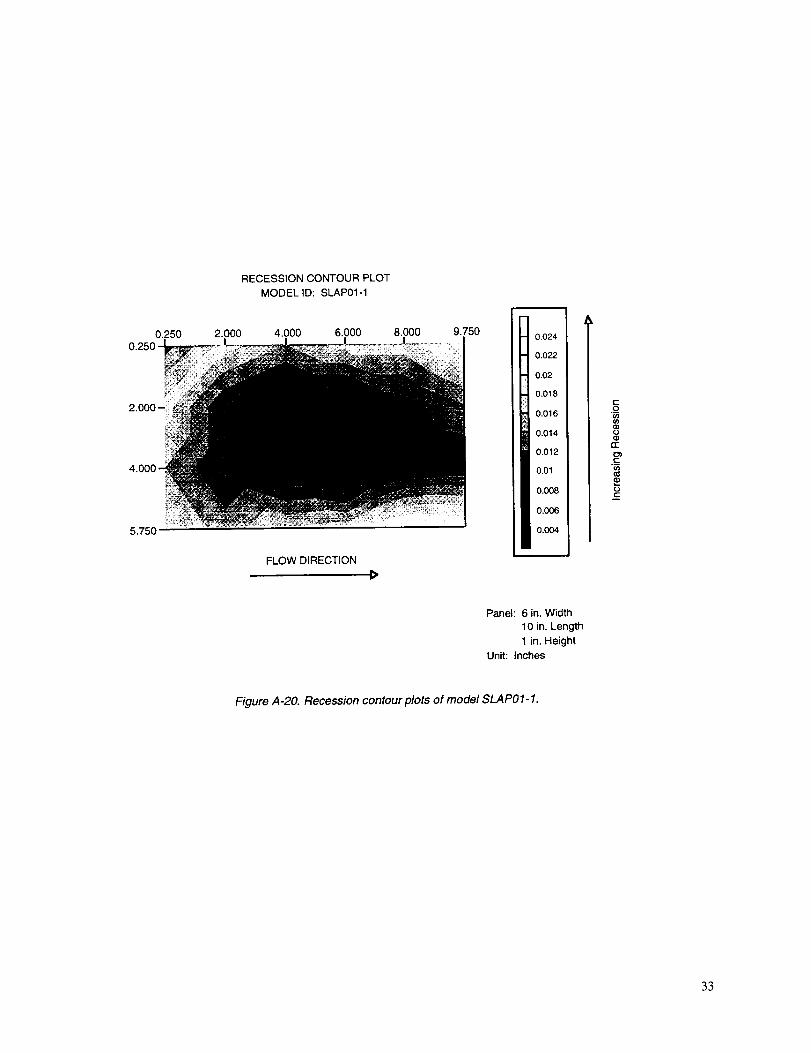
However, there were significant differences in surface

recession at each test condition. The sample tested at

Condition I had an average recession of about 0.034 cm,

about 0.041 cm for samples tested at Condition II, andabout 0.054 cm for Condition IH. A common feature

observed in samples from all three conditions was the

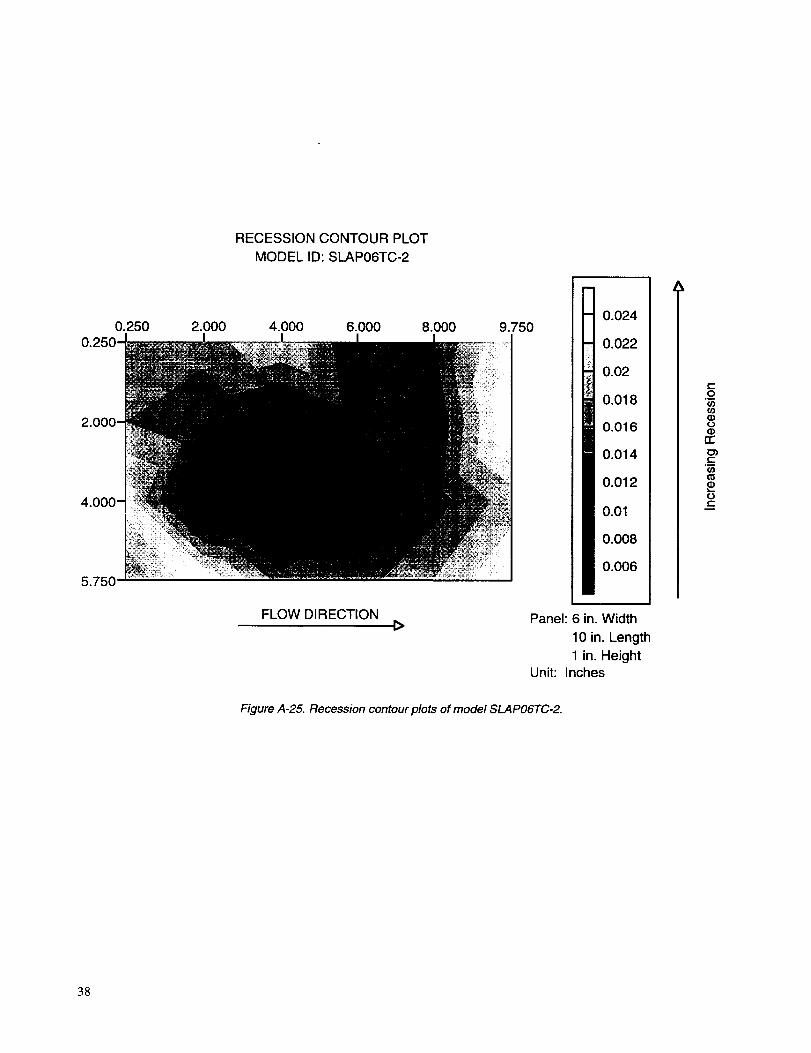
comparatively higher recession near the outer edges thanin the center. This is illustrated in the recession contour

plots for each model in Appendix A. Note that sampleSLAP04-3 had a slightly higher recession at the edges

than the other samples tested at the same Condition III,

because some flow penetrated into a narrow gap betweenthe model and frame.

Repaired Models

Model illustrations and labels are given in Appendix A.

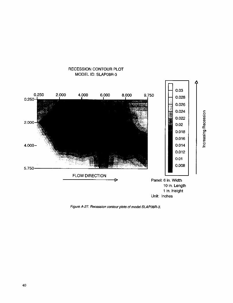
SLAP08R-3- This model, illustrated on page 18 of

Appendix A, had four repair plugs, each covering

0.07

0.06

oE 0.05

e

"i0.0, ,2,,,'r- 0.03¢D

=>0.o2.<

0.01

0 ' •

900O

(a)

• 13

1 #5, I'mlf4!_(_ • illl • ii 10

• J9

• #8

;I35.0

30.0

25.0

- 20.0

_1

• #1ol#'l

#7

l _ •

112

15.0

10.0

5.0

9000 11000

1 l_3, h_-m<xkd

11000 13000 15000 17000 19000 13000 15000 17000 19000

Time Integrated Shear Load, N.sec/m 2 Time Integrated Shear Load, N.sec/m 2

Co)

Figure 5. (a) Average recession vs. integrated shear load, (b) total mass loss vs. integrated shear load.

0.07

0.06

E 0.05

¢:._o

0.o4

_ 0.058,

o.o2

0.01

(a)

• #'3, troll-model

.mel_

• #1

•#4

iBI3

8#11 •#10

1119• #8

• #7

• #10 • 14 • #7113

35.0 _,

30.0 -E

I]B!6 • 111

25.0 -_

E _

_20.0 ÷

15.0 .1: m_._,_od_

lO.O .1:r

5.0 .._

r

o.o I .... : -

1500 1700

0 .... : .... : .... : .... : " " " ' " " " : .... : .... : , , , ,

1500 1700 1900 2100 2300 2500 1900 2100 2300 2500

Time Integrated Heat load, J/cm 2 Time Integrated Heat load, J/cm2

fo)

Figure 6. (a) Average recession vs. integrated heat load, (b) total mass loss vs. integrated heat load.

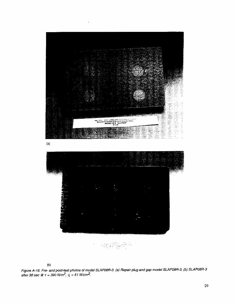
approximately 9 cells (3 x 3 cells). A filled gap, 0.076 cm

wide, ran completely across the model perpendicular to

the flow. All four plugs experienced cracking; this was

most extensive on plugs #2 and #3. A significant amountof material was removed by spallation and vaporization,

and large cracks appeared on these two repair plugs. Thesurfaces of all plugs inflated (rose above the surrounding

surface) to an average of about 0.13 cm; the inflation is

plotted in figure 7. The gap filler material melted, forming

a forward-facing step to the flow. This step increased the

local heating and material erosion near the center of themodel.

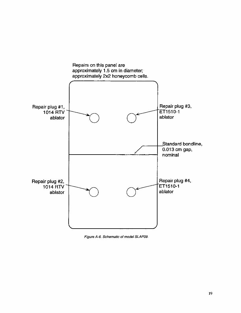
SLAP09R- This model, illustrated on page 19 of

Appendix A, had four repair plugs, each covering

approximately 4 cells (2 x 2 cells). It also had a gap,described by Lockheed-Martin-Michoud as a "standard

bondline" gap, running perpendicular to the flow. This

gap, nominally 0.013 cm wide, performed very well; no

significant enlargement, melting, or erosion was observed.

As in the SLAP08R model, all four repair plugs experi-

enced cracking and inflation. However, as figure 8 shows,

repair plugs #1 and #3 (the upstream plugs) experiencedmore inflation than plugs #2 and #4 (the downstream

plugs).

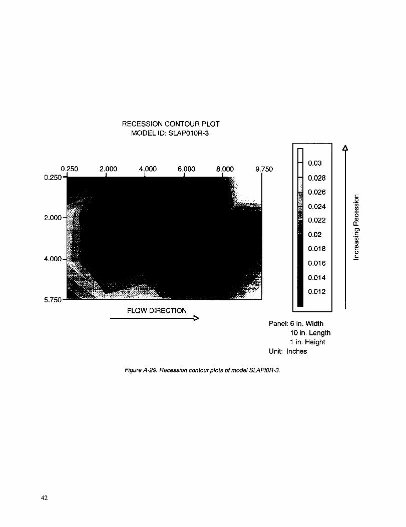
SLAP10R- This model, illustrated on page 20 of

Appendix A, had two gaps running the length of themodel, parallel to the flow direction. One was a standard

bondline gap and the other was a 0.076 cm wide gap filled

0.16.o.16:o.14i0.12 i

0.1

0.080.06

0.04

-0.02#1, 1014 RTV #2, 1014 RTV

Jl. lol4m_' I _2. 1014RW

#3, ET1510 #4, ET1510

0 °- Top

-Left w__ Right

180o-B0tt0m

Figure 7. Surface inflation measurements around repairson mode/SLAPO8R.

0.16.

0.14 -

0.12.

Eo 0.1-

._ 0.06-

_ 0._.

0.04.

0.02.

0#1. 1014 RTV

#3. ET1510-1

0

Jl I Io_4 m'v

I I

I I

#2, 1014 RTV #3, ETlSl0

114,ET1510-1

OSLAP09R-3

(9

#21 1014RTV

#4, ET1510

0"- Top

_22_'_r_1_1-I 90*-

.Left ¢,= _7--J _ Righl

180*-Bottom

Figure 8. Surface inflation measurements around repairson mode/SLAPO9R.

with GX-6300 resin. As in the prior test, the standard

bondline was essentially unaffected by the hot gas. The

0.076 cm gap was widened by flow penetration and meltrun-off was observed near the gap surface. Unlike the

SLAP08R model, surface erosion or material depletionwas not increased.

SLAPllR- This model, illustrated on page 21 of

Appendix A, had four repair plugs. The two upstream

repairs covered approximately 9 cells (3 x 3) and the othertwo covered approximately 4 cells (2 x 2). The repair

plugs #1 and #2, shown on the left in the figure, weremade of SLA-561V, including the honeycomb reinforce-ment, bonded with GX-6300. These plugs performed well,

recessing 0.05 cm, and no cracking was observed. The

downstream repair (plug #2) did not perform as well as

the upstream repair plug, however, because the inserted

core fit poorly into the opening. Repair plugs #3 and #4,

shown on the right in the figure, had honeycomb cores

hand-packed with ET1510-I resin. These repair plugs

experienced some cracking and inflation. Cell size did not

seem to have a significant impact on the repair perfor-

mance. Figure 9 shows that repair plugs filled withET1510-I inflated about 0.038 cm.

In-depth Temperature Response

Three models were instrumented with a total of 45 ther-

mocouples at various locations and depths to obtain tem-

perature contours and thermal response histories. Onemodel was tested at Condition II, the other two were

tested at Condition IU. with different test durations. Due

to limitations of the facility instrumentation, some of the

0.08

0._-

0.04-

0._°

g o-0.0_.

°0.04.

•0.06.

-0.08

I I I

#1, SLA561V #2, St.A561V

I113, ¢oqo _1510-1 114, COl_ _#q_-r 151 o. I

(3 °F-_- I SLAPIIR-3

B

© oI I1, SLA-561V 12. SL_561V

I#3, core with #4, core with

ET1510 0o. T E-r1510

.Left I¢_1_ L.I Right

180*-Bottom

Figure 9. Surface recession measurements around repairson model SLAP11R.

thermocouples were connected to a strip chart recorder.

Thirty-one thermocouples, or about 70 percent, produced

usable data. The figures in Appendix A (pages 15-17)

show the location and depth of each model's thermocou-

pies. Figures 10(a) and (b) show the in-depth temperature

response after 31 sec of exposures to Condition III, while

figures 1 l(a) and (b) show a typical response after 48 sec

of exposure. The temperatures indicated in figures 10(a)

and (b) are smooth, while those in figures 1 l(a) and (b)show some noise. The 5 to 7 percent variation in the peak

temperatures recorded by the gages installed 0.25 cmbelow the surface probably reflects primarily the variation

of heating rate over the model.

400

375 -

350-

E 325I.-.-

300

275

(a)

--TIC 8, O 1.27 cm depth

T/C 7 @ 1.27 cm depth

rJ

800

700 -

600-

500-

I- 400-

300-

' 2_ ' 45o " _o e6o lobo'1:/oo'_,_o 2OOo.... _oo'.... 2oo'...................._o ,_o s_o 66o 700Time, Sec.

Co)Time, See.

Figure 10. (a) In-depth temperature response to 31 sec exposure, from model SLAPO5TC-3, (b) in-depth temperature

response to 31 sec exposure, from mode/SLAPO5TC-3.

1200 . 1000

&E

1000-

800-

600-

400_

200

-- T/C 14. @ 0.25cmdep_

------ T/C 16. @ 1.27 cm dep_

i i i i i i i i , i = i i = i i ....

Tin'le, _

_2

I--

(a) Co)

f A i T/C 1, @ 0.25 cm depth

800.[ / _ ------TIC 2, @ 1.27 cm clep_

200 ] i i I i i i

0 100 200 300 400 500 600

Tir'Ne, Sec

Figure 11. (a) /n-depth temperature response to 48 sec exposure, from mode/SLAP07"I-C-3, (b) in-depth temperature

response to 48 sec exposure, from mode/SLAP07-1"C-3.

70O

Concluding Remarks

A total of eleven fiat panel models of SLA-561V ablativematerial were tested in the arc-heated Turbulent Duct

Facility. Three of the models were instrumented with

thermocouples and four others contained a variety of

repair plugs, gaps, and seams. The objective of the current

test was to expose the ablating SLA-561V to more

realistic shear stresses acting over a larger area than had

been possible during the previous arc-jet facility tests

performed at ARC during the November 1993 through

January 1994 time period. The non-ablating surface shear

stresses in the current test series ranged from being about

8 to 250 percent higher than the peak flight value, but the

corresponding test heating rates were only about 30 to

70 percent, respectively, of the maximum flight rates, due

to facility limitations. However, the peak flight values of

shear and the accompanying heating rate occur only over

a very small fraction of the forebody's surface, near the

rim or outer skirt region of the vehicle.

The over-all conclusion from the present test series is thatthe SLA-561V ablator exhibited no excessive char

removal or spallation. Even at the most severe shear test

condition, which exceeded the flight shear level by250 percent, the char remained intact, thus preserving its

ability to re-radiate heat. Although the test heating rates

were less than the peak flight rates, the SLA-561V should

withstand the shear stresses that are expected during

entry.

The only heat shield repair method that was effective in

the tests was to embed the resin in a phenolic honeycomb

core plug to protect the filler from excessive erosion. The

standard bondline gaps of 0.013 cm width withstood thetest environment well. In contrast, the filler used on the

wider, 0.076 cm gaps, melted or vaporized to a significant

depth, and caused the seams to widen.

Of the total of 45 thermocouples embedded in three mod-

els, 31 yielded usable data. Hopefully, this 70 percent

success rate can be improved in future tests. However, the

ability to obtain reliable thermocouple data in arc-jet facil-

ities remains a potential problem.

10

APPENDIX A

Appendix A

Thermocouple cross-reference table, model figures, model pre- and post-test photos, and recession contour plots.

The following table lists the thermocouples in the three instrumented models which produced valid data, available for

further analysis. Those thermocouples not listed here produced invalid or suspect data, due to ground loops, shorts,

inadequate shielding, or other instrumentation problems. The depth of the thermocouple from the surface is given; themodel illustrations on the following pages detail each thermocouple's location within the model.

Table A-1. Thermocouple data and model cross reference

Model ID T/C no. Depth, cm Model ID T/C no. Depth, cm Model ID T/C no. Depth, cm

SLAP05-1 0.25 SLAP06-2 0.25 SLAP07-2 0.25

SLAP05-2 0.25 SLAP06-5 0.25 SLAP07-3 0.25

SLAP05-3 0.25 SLAP0_6 0.25 SLAP07-5 0.25

SLAP05-4 0.25 SLAP06-10 0.25 SLAP07-6 0.25

SLAP05-5 0.25 SLAP07-7 1.27

SLAP05-6 0.25 SLAP07-9 2.54

SLAP05-7 1.27 SLAP07-10 0.25

SLAP05-9 2.54 SLAP07-11 1.27

SLAP05-10 1.27 SLAP07-12 1.91

SLAP05-11 1.27 SLAP07-13 2.54

SLAP05-12 2.54 SLAP07-14 0.25

SLAP07-15 2.54

SLAP07-16 1.91

SLAP07-17 1.27

SLAP07-19 1.91

SLAP07-20 2.54

13

33.0 cm 25.4 cm

I: ............................ I: ....

r: : : MmJr_tihgFrame, reusable " : : : : I: ....I: " " surface insulation (RSI) ; ; ; ;1: .....I............................. I.... .;

I< 15.2 cm "'=r I

<:: 20.1 cm + .0 :>".2

\0.64 cm R, 4 pl

Figure A-1. Schematic of models SLAPOI,SLAP02, SLAP03, and SLAP04.

]4

#123456

2.5 cm

3.8 cm

1

_-_ 7.6 cm _ 12

_,_ol_j1

1.3 cm (typ) ----_

8 1.3 cm (b/p)E- _ --.- x-

-_.Ec_-r___ _ _- -I I _ 2.5 cm, I

0"64 cm R' 4 Pt/L( 15.2 cm

J

Thermocouple depthbeneath surface

P-m

0.250.250.250.250.250.25

789101112

P..m

1.31.32.51.31.32.5

Figure A-2. Schematic of model SLAP05.

I)

..... ,-0

D

B _ •

E--

Aluminum

backplate,/ 0.64 cm

thk_k,nominal

]5

25.4 cm

15.2 cm

2.5 cm

15.1cm

r<------ 7.6cm_----_

I 2

" ' I

I

____ is

1.3 cm (typ) 7_ .1,____._e_ _ _

t°II I

t II/

1.3 cm (typ)--_l/

I t13

tII

i_3 _ _

J

I-->7 2.5 cm


cm #0.25 70.25 80.25 90.25 100.25 111.3 12

13

cm

0.251.90.250.251.31.90.25


2.5 cm

)

5.1 cm

5.1 cm

Aluminum

backplate,

thick,nominal

]6

25.4 cm

R

2.5 cm

t5.1 c_

7.6 cm

I 2--o-1 ---e

2.5 cm

.J_.,-- __ __ m

1.3 cm (typ)

e201 e18 i

t9 --_ 2.5cmj

IrIJ

-_-4 _._8

i i7I II H7

_1_ __.__

1.3 cm (typ)J _5_

I II i13

rJ

I

2°5 cm

.)

1

2

3

4

5

6

7

8

9

10


cm #

0.25 11

0.25 12

0.25 13

0.25 14

0.25 15

0.25 16

1.3 17

1.9 18

0.25 19

0.25 20

cm

1.31.92.50.252.51.9

1.3

1.3

1.9

2.5

Figure A-4. Schematic of mode/SLAP07.

! •

i5.1 cm

-- D--•

q

5.1 cm

l?

Repair plug #1,1014 RTV

ablator

Repair plug #2,1014 RTV

ablator

Repairs on this panel areapproximately 3.3 cm in diameter;approximately 3x3 honeycomb cells.

Figure A-5. Schematic of mode/SLAP08.

Repair plug #3,IET1510-1

ablator

0.076 cm gap filledwith GX6300adhesive

Repair plug #4,""ET 1510-1

ablator

18

Repair plug #1,1014 RTV -

ablator

Repair plug #2,1014 RTV-

ablator

Repairs on this panel are

approximately 1.5 cm in diameter;

approximately 2x2 honeycomb cells.

/


Repair plug #3,"ET1510-1

ablator

Standard bondline,

0.013 cm gap,nominal

Repair plug #4,ET1510-1

ablator

19

0.076 cm gap filledwith GX6300 adhesive

!

J

q

Figure A-7. Schematic of mode/SLAPIO.

Standard bondline,0.013 cm gap,nominal

2o

Repair plug #1,SLA-561V

core plug,bonded with

GX6300

Repair plug #2,SLA-561V

core plug,bonded with

GX6300

Diameter approx.3.3 cm, 3x3 cells.

Repair plug #3,1honeycomb

core hand-

packed withET1510-1

ablator

Repair plug #4,

lhoneycombcore hand-

packed withET1510-1

ablator


21

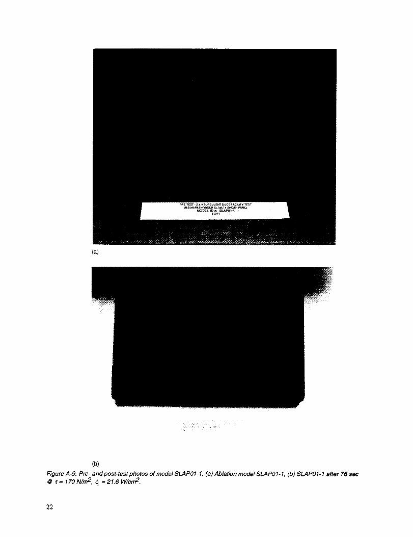
(a)

Figure A-9. Pre- and post-test photos of model SLAP01-1. (a) Ablation model SLAP01-1, (b) SLAP01-1 after 76 sec@ _= 170 N/m 2, q = 21.6 W/cm2.

22

(a)

Figure A- 10. Pre- and post-test photos of model SLAP02-2. (a) Ablation model SLAP02-2, (b) SLAP02-2 after 39 sec

@ _ = 240 N/m 2, c] = 40 W/cm 2.

23

(a)

. _ i,_,_ , i, .... i ' ,_11•

Co)


@ _ = 390 N/m 2, (] = 51 W/cm 2.

24

(a)

_)


@ • = 390 N/m 2, q = 51 W/cm 2.

25

(a)

MODEL IO ,=: SLAPOS-"N

(b)

Figure A- 13. Pre- and post-test photos of model SLAPO5TC-3. (a) Instrumented model SLAPO5TC-3, (b) SLAPO5TC-3

a_er 31 sec @ • = 390 N/m 2, q = 51 W/cm 2.

26

(a)

Figure A- 14. Pre- and post-test photos of model SLAPO6TC-2. (a) Instrumented model SLAPO6TC-2, (b) SLAPO6TC-2

after 38 sec @ T = 240 N/m 2, cl =40 W/cm 2

2?

(a)

,_.! i, .i,!,i_i_Ji_¸ /i! i _' ,'_,,i, ¸¸.'i "

_)

Figure A- 15. Pre- and post-test photos of model SLAP07"I-C-3. (a) Instrumented model SLAP07-I-C-3, (b) SLAP07-I'C-3

after 48 sec @ • = 390 N/m 2, (] =51 W/cm 2

28

(a)

: _,,_,i_,i!_ill ¸¸ ,/iii_i _:.i_i__

_)

Figure A- 16. Pre- and post-test photos of model SLAPO8R-3. (a) Repair plug and gap model SLAPO8R-3, (b) SLA PO8R-3

after 38 sec @ • = 390 N/m 2, (] = 51 W/cm 2

29

(a)

............i_I _. ,_

Co)

Figure A-17. Pre- and post-test photos of model SLAPO9R-3. (a) Repair plug and gap model SLAPO9R-3, (b) SLAPO9R-3after40 sec @ _ = 390 N/m 2, q = 51 W/cm 2

3O

(a)

._ _, _Y' -i̧ : ,i_' _i.'.i _

(b)

Figure A- 18. Pre- and post-test photos of model SLAPIOR-3. (a) Gap model SLAPIOR-3, (b) SLAPIOR-3 after 38 sec

@ • = 390 N/m 2, ct = 51 W/cm 2

3]

(a)

", _ _ i,_ _'_ 'i

(b)

Figure A-19. Pre- and post-test photos of model SLAPIIR-3. (a) Repair plug model SLAP11R-3, (b) SLAP1 IR-3 after36 $ec @ • = 390 N/m 2, (] = 51 W/cm 2

32

RECESSION CONTOUR PLOT

MODEL ID: SLAP01-1

5.75O

0.250 2.000 4.000 6.000 8.000 9.750

FLOW DIRECTION

N 0.024 I

H::IHo.o,oIH0.0,4Ii 0.0,2I

ilO.O,i11o.oo8/ilO._Oiiao- /

e.-

ilJ

I-

Q)

u

Panel: 6 in. Width

10 in. Length

1 in. Height

Unit: Inches

Figure A-20. Recession contour plots of model SLAPO 1-1.

33

RECESSIONCONTOURPLOTMODELID:SLAP02-2

0.250 2.000 4.000 6.000 8.000 9.750

2.000

4.000

5.750

FLOWDIRECTIONb.

0.030.0280.0260.024

0.0220.020.0180.016

0.0140.0120.010.0080.006

Panel:6 in.Width10in.Length1in.Height

Unit: Inches

E.o(/)(/)

o

rr

(-

.e(3(-

Figure A-21. Recession contour plots of model SLAP02-2.

34

RECESSIONCONTOURPLOTMODELID:SLAP03-3

0.250 2.000 4.000 6.000 8.000 9.750

5.750

FLOWDIRECTION!>

Unit:

Figure A-22. Recession contourplots of model SLAP03-3.

0.03

0.028

0.026

0.024

0.022

0.02

0.018

0.016

Panel: 6 in. Width

10 in. Length

1 in. HeightInches

4,.-o

(_t,f)

f3

rr

t-

¢-

35

0.250

2.000

4.000-

iiii

5.750

2.000I


MODEL ID: SLAP04-3

4.000 6.000 8.000 9.750

FLOW DIRECTION

0.03

0.028

0.026

0.024

0.022

0.02

0.018

0.016

Panel: 6 in. Width

10 in. Length

1 in. HeightUnit: Inches

¢-

.o_(/)(/)

(._

13:

¢-(t)

ecJ(.-

Figure A-23. Recession contour plots of rnodel SLAP04-3.

36

0.250

0.250 -J

2.000-

4.000

5.750


MODEL ID: SLAP05TC-3

2.000 4.000

I .......I

FLOW DIRECTION

0.024

0.022

0.02

0.018

0.016

0.014

Panel: 6 in. Width

10 in. Length

1 in. Height

Unit: Inches

t-O

°D

(/3C/)

¢c

c-°_

Ot-

Figure A-24. Recession contour plots of model SLAPO5TC-3.

3"7


MODEL ID: SLAP06TC-2

0.250 2.000 4.000 6.000 8.000 9.750

5.750

FLOW DIRECTION!>

0.024

0.022

0.02

0.018

0.016

0.014

0.012

0.01

0.008

0.006

Panel: 6 in. Width

10 in. Length


t-

.ococO(1)

rc03

(/)

Ot--


38

RECESSIONCONTOURPLOTMODELID:SLAP07TC-3

0.2500.250_ -

2.000 4.000 6.000 8.000I

2.000-

4.000 -

5.750_"_ .... ..... ..........

FLOW DIRECTIONE>

9.7500.03

0.028

0.026

0.024

0.022

0.02

0.018

0.016

0.014

Panel: 6 in. Width

10 in. Length


t-O

.m

Q)t3

¢r

t-

OC


39

RECESSIONCONTOURPLOTMODELID:SLAP08R-3

0.2500.25(

4.000-

5.750

2.000 4.000 6.000 8.000 9.750

FLOW DIRECTION

0.03

0.028

0.026

0.024

0.022

0.02

0.018

0.016

0.014

0.012

0.01

0.008

Panel: 6 in. Width

10 in. Length


t-O03_O¢D

tr"

¢-.

mt.-

Figure A-27. Recession contour plots of model SLAPO8R-3.

40

RECESSIONCONTOURPLOT/MODELID:SLAPO9R-3

0.250

5.750

2.000 4.000 6.000 8.000I I I

FLOW DIRECTION

9.7500.03

0.028

0.026

0.024

0.022

0.02

0.018

0.016

0.014

0.012

0.01

0.008

Panel: 6 in. Width

10 in. Length


oo--fltJ

n-

Figure A-28. Recession contour plots of model SLAPO9R-3.

4]


MODEL ID: SLAP010R-3

0.250 2.000 4.000 6.000

5.750

FLOW DIRECTION

8.000

b,

9.7500.03

0.028

0.026

0.024

0.022

0.02

0.018

0.016

0.014

0.012

Panel: 6 in. Width

10 in. Length


t-.o(/)(/]

ccc_t-

°_

t_eot-

Figure A-29. Recession contourplots of model SLAPIOR-3.

42

RECESSIONCONTOURPLOTMODELID:SLAP011R-3

0.250

5.750

2.000 4.000 6.000 8.000I I

FLOW DIRECTION

9.7500.03

0.028

0.026

0.024

0.022

0.02

0.018

0.016

0.014

0.012

0.01

Panel: 6 in. Width

10 in. Length


t-O(/)

rrE3(-.m(/)

(3t-

Figure A-30. Recession contour plots of model SLAP1IR-3.

43

Form Approved

REPORT DOCUMENTATION PAGE OMBNo0704-0188Public reporting burden for this collection of information is estimated to average I hour per response, including the time for reviewing instructions, searching existing data sources,

gathering and maintaining the data needed, and completing and reviewing the collection of information. Send comments regarding this burden estimate or any other aspect of this

collectio_ of information, including suggestions for reducing this burden, to Washington Headquarters Services, Directorate for information Operations and Reports, 1215 Jefferson

Davis Highway, Suite 1204, Arlington. VA 22202-4302. and to the Office of Management and Budget, Paperwork Reduction Project (0704o0188). Washington, DC 20503.

1. AGENCY USE ONLY (Leave blank) | 2. REPORT DATE 3. REPORT TYPE AND DATES COVERED

I September 1996 Technical Memorandum4. TITLE AND SUBTITLE 5. FUNDING NUMBERS

Ames Research Center Shear Tests of SLA-561V Heat Shield

Material for Mars-Pathfinder

6. AUTHOR(S)

Huy Tran, Michael Tauber,* William Henline, Duoc Tran,*

Alan Cartledge, Frank Hui, and Norm Zimmerman*

7. PERFORMING ORGANIZATION NAME(S) AND ADDRESS(ES)

Ames Research Center

Moffett Field, CA 94035-1000

9. SPONSORING/MONITORING AGENCY NAME(S) AND ADDRESS(ES)

National Aeronautics and Space Administration

Washington, DC 20546-0001

232-01-04

8. PERFORMING ORGANIZATIONREPORT NUMBER

A-961865

10. SPONSORING/MONITORINGAGENCY REPORT NUMBER

NASA TM- 110402

11. SUPPLEMENTARY NOTES

Point of Contact: Huy Tran, Ames Research Center, MS 234-1, Moffett Field, CA 94035-1000(415) 604-0219

*Thermosciences Institute, Moffett Field, California12a. DISTRIBUTION/AVAILABILITY STATEMENT

Unclassified-Unlimited

Subject Category - 05

12b. DISTRIBUTION CODE

13. ABSTRACT (Maximum 200 words)

This report describes the results of arc-jet testing at Ames Research Center on behalf of Jet Propulsion Laboratory (JPL) for the

development of the Mars-Pathfinder heat shield. The current test series evaluated the performance of the ablating SLA-561V heat shield

material under shear conditions. In addition, the effectiveness of several methods of repairing damage to the heat shield were evaluated.

A total of 26 tests were performed in March 1994 in the 2" x 9" arc-heated Turbulent Duct Facility, including runs to calibrate the facility

to obtain the desired shear stress conditions. A total of eleven models were tested. Three different conditions of shear and heating were

used. The non-ablating surface shear stresses and the corresponding, approximate, non-ablating surface heating rates were as follows:

Condition I, 170 N/m 2 and 22 W/cm2; Condition II, 240 N/m 2 and 40 W/cm2; Condition III, 390 N/m: and 51 W/cm 2. The peak shear stress

encountered in flight is represented approximately by Condition I; however, the heating rate was much less than the peak flight value. The

peak heating rate that was available in the facility (at Condition III) was about 30 percent less than the maximum value encountered during

flight. Seven standard ablation models were tested, of which three models were instrumented with thermocouples to obtain in-depth

temperature profiles and temperature contours. An additional four models contained a variety of repair plugs, gaps, and seams. These

models were used to evaluated different repair materials and techniques, and the effect of gaps and construction seams. Mass loss and

surface recession measurements were made on all models. The models were visually inspected and photographed before and after each

test. The SLA-561V performed well; even at test Condition III, the char remained intact. Most of the resins used for repairs and gap fillers

performed poorly. However, repair plugs made of SLA-561V performed well. Approximately 70 percent of the thermocouples yielded

good data.

14. SUBJECT TERMS

Planetary exploration, Thermal protection system, Space vehicle

17. SECURITY CLASSIFICATIONOF REPORT

Unclassified

NSN 7540-01-280-5500

18. SECURITY CLASSIFICATIONOF THIS PAGE

Unclassified

19. SECURITY CLASSIFICATIONOF ABSTRACT

15. NUMBER OF PAGES

4916. PRICE CODE

A0320. LIMITATION OF ABSTRACT

Standard Form 298 (Rev. 2-89)Prescribed by ANSI Std. Z39-18298-102

ames research center shear tests of sla-561v heat ... technical memorandum 110402 ames research...

Documents