A-AI81 394 INFERENCE AMD PREDICTION FOR A GENERAL ORDER STATISTIC I/iMODEL WITH UNKNOWN POPULATION SIZE(U) WASHINGTON UNIVSEATTLE DEPT OF STATISTICS A E RAFTERY AUG 86 TR-88

UNCLRSSIFIED N88814-84-C-8i69 F/G 12/3IlmmllllllllollllllllllolllllEl

128

% 4.0

JX.,

OTC FILE GO"

A U, -IS L : .. .

00 12

L' #f . -- + - € , , ., , .

i jA- *4'"* '.k

Jr.

loPo

I

ilIIi

S.o" oP w l l

SECURITY CLAS31FICATION OF THIS PAGE ("an D~a entered)

REPORT DOCUMENTATION PAGE REDISRCIN1. REPORT NUMBER 2. GOVT ACCESSION ml3. RECIPIENT'S CATALOG NUMBER

88Nj4. TITLE ( d Subtitle) 5. TYPE OF REPORT & PERIOD COVERED

Inference and prediction for a general order TR 12/86 - 6/88statisiic model with unknown population size 6. PERFORMING ORG. REPORT NUMBER

7. AUTHOR(s) a. CONTRACT OR GRANT NUMBER(e)

Adrian E. Raftery IN00014-84-C-0169

9. PERFORMING ORGANIZATION NAME AND ADDRESS T10. PROGRAM ELEMENT. PROJEC,. TASKDepartment of Statistics, GN-22 f AREA & ORK UNIT NUMBERS

University of Washington NR-661-003Seattle, WA 98195I

I I. CONTROLL.ING OFFICE NAME AND ADDRESS 12. REPORT DATE

ONR Code N63374 August 19861107 NE 45th Street 13. NUMBER OF PAGES

Seattle, WA 98105 -23

IA. MONITORING AGENCY NAME & AOORESS(If differoe froa, Controlling Office) IS. SECURITY CLASS. (of chi* report)

Unclassified

15a. DECLASSI FICATION/ DOWNGRADING

SCHEDULE

16. DISTRIBUTION STATEMENT (of this Report)

APPROVED FOR PUBLIC RELEASE: DISTRIBUTION UNLIMITED.

17. OISTRIB3UTION STATEMENT (of the abetrect enltered In Block 20, It different trogn Report)

IS. SUPPLEMENTARY NOTES

IS. KEY WORDS (Continue on, tera.s adeJ ineceaefa and Identify by block numiber)

Bayes empirical Bayes; Bayes factor; Non-nested models; Pareto orderstatistic model; Software reliability; Weibull order statistic model

20. AsS" RAC7 rContin.. ,n ra-so~ @#do It ieceery and identify by block nwrtber)Suppose that the first n order statistics from a random sample of N

positive random variables are observed, where N is unknown. A Bayesempirical Bayes approach to inference is presented. This permits thecomparison of competing, perhaps non-nested, models in a natural way, andalso provides easily implemented inference and prediction procedures whichavoid the difficulties of non-Bayesian methods. Applications to threesoftware reliability data sets indicate that the much-used / CONTINUED ...

D D I JA 7 1473 EDITION OF I NOV 65 13 OBSOLETE

5,,N 0102.. 0 QJ- 6601 SECURITY CLASSIFICATION OF THIS P&GE 'When Dc,. 3-n0100)

-~ -j ?1 v,-. .~ ~'

exponential order statistic model may give rather optimistic estimates

of system reliability, while the, not previously considered, Weibull order

statistic model seems promising for such applications.

-A-4

U,

6

Inference and Prediction for a General Order Statistic Model WithUnknown Population Size

Adrian E. Raftery

Department of Statistics, GN-22,University of Washington,

Seattle, WA 98195.

ABSTRACT

Suppose that the first n order statistics from a random sample of N positiverandom variables are observed, where N is unknown. A Bayes empirical Bayesapproach to inference is presented. This permits the comparison of competing,perhaps non-nested, models in a natural way, and also provides easilyimplemented inference and prediction procedures which avoid the difficulties ofnon-Bayesian methods. Applications to three software reliability data setsindicate that the much-used exponential order statistic model may give ratheroptimistic estimates of system reliability, while the, not previously considered,Weibull order statistic model seems promising for such applications. A.' , .,r

KEY WORDS: Bayes empirical Bayes; Bayes factor; Non-nested models; Pareto order statisticmodel; Software reliability# Weibull order statistic model.

Akce3ion For

NTIS CRA&

D iC TAB U,,jr -.ou r.cd "J J1q'tFcat10'o....J

IByi.. . . ....... . . . . . .

D't!b ;ti"/'

i,:XIJ'y Cc,4e si A I -,j or

Adrian E. Raftery is Associate Professor of Statistics and Sociology, University of Washington,Seattle, WA 98195. This work was supported by the Office of Naval Research under contractN00014-84-C-0169. I am grateful to W.S. Jewell for helpful discussions, and to Peter Guttorp forhelpful comments on an earlier version of this paper.

p IIJIm

-2-

1. INTRODUCTION

Suppose X 1, ... , XN is a random sample of positive random variables from a distribution

with probability density function (pdf) at x equal to 3f 0(4). Here 0 is a scalar precision

parameter, 0 is a, possibly vector, shape parameter, and N is unknown. In applications, Xi is

often a length of time, such as a lifelength, and Xi =x corresponds to the occurrence of an event

at time x. I shall use this temporal imagery without further explanation.

The first n order statistics, t =(t 1 .... t), are observed, where 0!5t 1 ". t, <T. T is

the period of observation: there is no Xi such that t, <X i5 T. Inference is to be made about the

unknown parameters, and future observations are to be predicted.

I shall call this the general order statistic (GOS) model. Special cases have been proposed

as models for market penetration and capture-recapture studies (Anscombe 1961), bum-in in

repairable systems (Bazovsky 1961, chap. 8; Cozzolino 1968), software reliability growth

(Jelinski and Moranda 1972; Littlewood 1981), estimating the number of individuals exposed to

radiation (Hoel 1968), and estimating the number of unseen species (Efron and Thisted 1976,

and references therein).

Perhaps the simplest special case is the exponential order statistic (EOS) model where

f 0 (x )=exp(-x), statistical analysis of which has been extensively studied (Blumenthal and

Marcus 1975; Forman and Singpurwalla 1977; Goudie and Goldie 1981; Jewell 1985; Joe and

Reid 1985; Raftery 1986a). It has been used extensively as a simple, physical, debugging model

for software reliability. In this context it is often called the Jelinski-Moranda model, and is based

on the assumption that a system has N faults, each of which causes a failure of the system, and is

-- -- - - --

-3-

then located and removed; the times at which the N failures occur are independent and

identically distributed exponential random variables. However, the examples in Section 6 show

that it may give rather optimistic estimates of system reliability.

The EOS model can be generalised by assuming that X 1... ,X. are independent

exponential random variables with different means 4-1,... , where 41, ... N is itself a

random sample from a distribution with pdf at equal to 1we(3-1 ). This is a special case of

the GOS model, where

fe(x) =y w(y) exp(-xy) dy (1.1)

Miller (1986) has pointed out that many proposed software reliability models are, in fact, of this

form. When the 4i have a gamma distribution, the Xi have a Pareto distribution. This, the

Pareto order statistic (P0S) model, is discussed in more detail in Section 5.2.

I adopt a Bayes empirical Bayes approach (Deely and Lindley 1981) to the problem of

inference for the GOS model. This has the advantage of permitting comparisons between

competing, perhaps non-nested, models for f e(x) in a natural way (Section 2), as well as

providing easily implemented inference and prediction procedures which avoid the difficulties of

non-Bayesian methods (Section 3). One such difficulty is that the maximum likelihood estimator

of N may be infinite. Indeed, Goudie and Goldie (1981) concluded that for the special case they

considered, all standard non-Bayesian point estimation techniques are liable to fail. Attention is

paid to the situation where vague prior information about the model parameters is approximated

by limiting, improper, prior forms.

.4l'111 1W.J.M M

-4-

Some analytic simplification is possible for the Weibull order statistic (WOS) model, where

the Xi have a Weibull distribution (Section 5.1). The examples in Section 6 suggest that this

model may be promising for software reliability applications, for which it has not previously

been considered.

2. MODEL COMPARISON

Consider the GOS model described in Section 1. In this section and the next one I assume

that 0 is known and omit it from the notation; this assumption is relaxed in Section 4. I assume

that N has a Poisson distribution in the GOS model; this defines an empirical Bayes model in the

sense of Morris (1983).

It is equivalent to a non-homogeneous Poisson process with X(s), the intensity function at

time s, given by X(s) = pf (13s) (p>O). The likelihood is

np (t I p3) = pn { 1f (Pti)}exp{-p0-1F(PT)} (2.1)

i=1

where F (x) = f (y) dy.0

Consider the problem of comparing competing, perhaps non-nested, models for f (x), M

and M 2, say. Such comparisons will be based on the Bayes factor, or ratio of posterior to prior

odds for M I against M 2,

B 12 =p(t IM 1)/p(t IM 2) (2.2)

the ratio of the marginal likelihoods. In (2.2),

-5-

p(t IM)= f p(t Ip,lMi)p(pPIMj)dpd P (i=1,2) (2.3)0 0

If the priorsp(pPjIM) (i=1,2) are proper, (2.2) can be evaluated directly.

I now develop an expression for B 12 in the situation where vague prior knowledge is

approximated by limiting, improper, prior forms. This is done by comparing M 1 and M 2 in turn

with the constant rate Poisson process, M 0 : X(s) = p., which is nested within each of M 1 and M E.

This yields Bayes factors B 0 1 and B 02, where

Boj =p(t 1Mo)/p(t IMi) (i=1,2) (2.4)

*" and

p(t IMo)= fp(t Ig,Mo)p(.IjM o)dp. (2.5)0

Then B 12 = B01 B . Comparison of M 0 with Mi using (2.4) may itself be of interest. For

example, in the software reliability context, it provides a test of whether the system is, indeed,

being debugged.

I use the standard vague prior for gt,

p(t M 0 ) = c0- 1 (2.6)

(Jaynes 1968), and consider the evaluation of B 01. In order to provide a satisfactory

approximation for vague prior knowledge over all scales, the prior distribution of (p,3) should

yield a Bayes factor B 01 which is time-invariant, i.e. invariant to scale changes in the time

variable.

1le

-6-

Theorem 1: B o1 is time-invariant if and only if there is a function (.) such that

p (pD3IM 1) = c lp-2(p-l3) (2.7)

Proof. Suppose B 01 is time-invariant. By (2.6)

p (t I M0) = co(n-1)! T" (2.8)

Using (2.1), and substituting pT for p and 3T for P3 in (2.3), and then dividing the result into

(2.8), yields, by (2.4),

B 01 = c 01 [f f pn {If (Dui) exp{-p3-1F (P)I T- 2p (pT-',PT-'I M 1) dpd P]- (2.9)00 i=1

Thus

T- 2p (pT-l,3T-I M 1) =p(pP3IM 1) (p,D3,T>0) (2.10)

Setting T=p in (2.10) yields (2.7), where O(x)=p(p=l,-x IMI). Also, when (2.7) holds, the

time-invariance ofB 0 1 follows by direct substitution in (2.9). This completes the proof.

If the prior is to be asymptotically non-increasing in p and 3, then, by Theorem 1, O(x)

must be bounded above by yl and below by y2x - 2 for x sufficiently large, where y and y2 are

positive constants. Consider now the case where the likelihood (2.1) is of exponential family

form, so that

J d

f13x) = exp {a (3) + a (x) + Y (Ox) dJ+ const.} (2.11)j=1

This is quite a general family, and includes, for example, the gamma and Weibull distributions.

By (2.1), a natural family of conjugate prior distributions is

'I

-7-

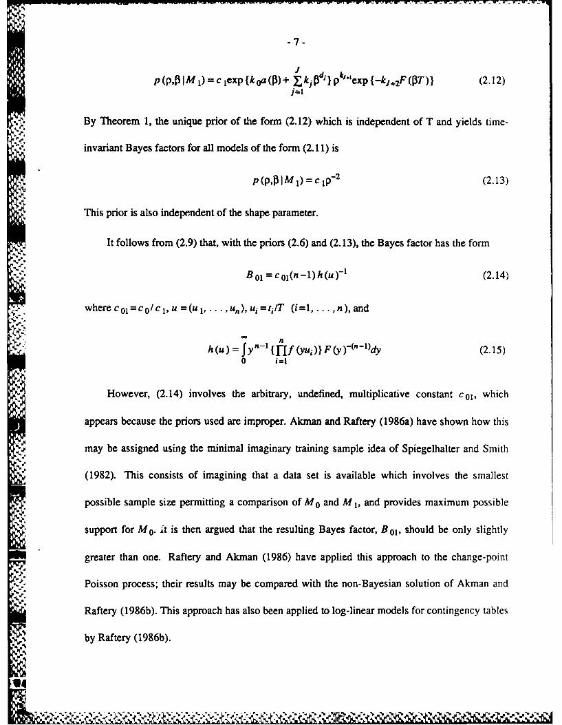
p (p I M1 ) = c jexp {koa (13) + 'k,} pkJ'exp {-kj+ 2F (13T)} (2.12)j=1

By Theorem 1, the unique prior of the form (2.12) which is independent of T and yields time-

invariant Bayes factors for all models of the form (2.11) is

p (p,13IM 1) = c 1 p- 2 (2.13)

This prior is also independent of the shape parameter.

It follows from (2.9) that, with the priors (2.6) and (2.13), the Bayes factor has the form

B 01 = c 01(n -1) h (u)-1 (2.14)

,,.where col=colcl, u =(ul .. ',) itl il...nd

h(u) = Jy -1{If(yui)}F(y)-(n-1 )dy (2.15)0 i=1

However, (2.14) involves the arbitrary, undefined, multiplicative constant col, which

appears because the priors used are improper. Akman and Raftery (1986a) have shown how this

may be assigned using the minimal imaginary training sample idea of Spiegelhalter and Smith

(1982). This consists of imagining that a data set is available which involves the smallest

possible sample size permitting a comparison of M0 and M 1 , and provides maximum possible

support for M0 . it is then argued that the resulting Bayes factor, B0 1, should be only slightly

greater than one. Raftery and Akman (1986) have applied this approach to the change-point

Poisson process; their results may be compared with the non-Bayesian solution of Akman and

Raftery (1986b). This approach has also been applied to log-linear models for contingency tables

by Raftery (1986b).

'14

.4%-. Z

-8-

In the present situation, the appropriate imaginary data set consists of two observations at

the same value, u = (u 1,u 2) = (,1), where 'u is chosen so as to maximise the value of B 01 in

(2.14). In practice, in all the examples considered, B 01 is maximised at either u= or u=O. When

B 01 is maximised at u=0, however, the maximum value is infinite. In such cases, I use the local

maximum at ij=l, because this corresponds, in the software reliability situation, for example, to

the data set which suggests most strongly that the system is not being debugged. This yields

c01 yf (y)F (y) (2.16)0

Strictly speaking, any value of B 12 less than one suggests that the data provide evidence

against M1 for M 2. However, as a rough order of magnitude interpretation, Jeffreys (1961,

Appendix B) has suggested that the evidence should be regarded as strong only if B 12< 10- 1,

and as decisive only ifB 12< 10- 2.

3. ES, iMATION AND PREDICTION

I now consider estimation of N, and prediction of future observations for the GOS model.

The framework developed in Section 2 is used. It follows from (2.13) that

p (N ,) J p (N Pp3) p (p,)d p0

" {N (N-I)}--' (3.1)

"-d Also,

,, m -..- m a , p, , -' -.-. a,- lM L. /' '€.-. . . . ', '.- ". , - - : . ._, ,.':'": ,--..',.

~- 9-- 7-7.

n- p(t 1N,3) = {N!I(N-n)!} ' {'1f (ti)}j(3T)N - n (3.2)

where F(x) I -F (x). Combining (3.1) with (3.2) and integrating over I3 yields the posterior

distribution of the number of unobserved variables M =N-n,

,:.,:. p(M It) {(M+n-2)!/M!}g(uM) (M=0,1,'-') (3.3)

where

g(u,M) = y Il f(Yuj F(y)M dy (3.4)

Point estimators of N may be obtained by combining (3.3) with an appropriate loss

*f function; examples are the posterior mode and the posterior median. However, experience with

the simple EOS model indicates that point estimators of N are liable to perform badly (Raftery

1986a). Interval estimators of N, such as highest posterior density regions, can readily be found

from (3.3), and may well be more useful.

"4 Various prediction problems may be of interest, and can be solved, often quite easily, using

the present approach. One example is finding the probability, given the data, that there is no Xi

such that T <. Xi < T+z. In the software reliability context, this is the current reliability of the

system for a task of length z. IfZ =tn, 1-T, where tN+1=*, then

P[Z>zlt]= I JP[Z>z ltlp(MIlt)dpM=00

=P[M--OIt]+{T/(T+x)} , {g(uT/(T+x),M)/g(u,M)}p(M t) (3.5)M=I

o ..j

4° -°.

0;:;:-;:' ,6 ,),-.:) :: :.- .:::.- ::,.;::::, -,-.:: :. :.:o::::'.,;, . *: ,; ; - : ;

-10-

4. SHAPE PARAMETER UNKNOWN

Suppose now that the shape parameter 0 in the GOS model is unknown. I continue to use

the framework of Sections 2 and 3, but quantities which depend on 0 are now written with a

subscript 0. I know of no single prior which can provide a satisfactory approximation for vague

prior knowledge about 0 in all situations. I therefore assume that

p (pO3,) = c IP-2P (0) (4.1)

where p (0) is proper. I denote the set of possible values of 0 by E.

The results of Sections 2 and 3 can be generalised to this situation by conditioning on 0 and

using the total probability law in an appropriate way. Thus (2.14) becomes

B 0 1 = C0 1(n-1)H(u)- 1 (4.2)

where

H (u)= f h 0(u)p (0) dO (4.3)

and he(u ) is defined by (2.15). (2.16) becomes

Col = f f Yf e(y) 2 Fe(y )- 'dy p (O)d (4.4)00

For estimation of N, (3.3) becomes

i whp(M It) {(M+n-2)!/M!}G(u,M) (M--O,1,...) (4.5)

where

G(u,M)=fg(u,M)p(0)d0 (4.6)9

L|

U and g 9(u A) is defined by (3.4).

For the prediction problem considered in Section 3, (3.5) becomes

V P[Z>z It] =P[MOItJ+T(T+x)M j {G(uT/(T+x),MYVG(uM)}p(M It) (4.7)M=1

5. SPECIAL CASES

5.1 The Weibull Order Statistic (WOS) Model

Among commonly used models for positive random variables, the Weibull distribution

yields some analytic simplification of the results in Section 4. The WOS model is defined by

setting

f8(x)=09'exp(-x9) (0>0)(.1

in the GOS model. Then 8 01 is given by (4.2), (4.3), and (4.4), where

hq(u) = 9'-1(juj)9-lexp(-y~uj6{yI(l&eY))4-1dy

and c0 )E[)

The solutions to the estimation and prediction problems are given by (4.5), (4.6), and (4.7).

where

g 1 ui), I Us+A

- 12-

5.2 The Pareto Order Statistic (POS) Model

Consider the POS model described in Section 1, where in (1.1),

we(Y) = r(r y-- e- (5.2)

so that, by (1. 1),

f 0(Y) = 0 (l+y)- 1"+ (5.3)

B 01 is again given by (4.2) and (4.3), where

he(u) = 0 f(1+13ui) - 1 ) Jy"- { 1-4+y )- }- -1) dyi=1 0

and (4.4) becomes

Cot jy (l+yf :., {1(I+y-)-,dy ,0()dO

The solutions to the estimation and prediction problems are somewhat simplified if a

gamma prior for 0 is used, namely, in (4. 1),

p (0) o 0OK- I e -*° (5.4)

aThe solutions are given by (4.5) and (4.7), where

G G(uM)ocf(41u 8 )l (KC2+ ilglyj+ lg~~)-nlldy

It Most of the integrals in this section, which require numerical evaluation, could be replaced

by convergent infinite series. However, this was not found to be computationally advantageous.

Ul

- 13-

6. EXAMPLES

I now apply the techniques proposed here to three, previously analyzed, software reliability

data sets.

Example 1: Goel and Okumoto (1979) gave the 31 failure times of a piece of software

developed as part of the Naval Tactical Data System. The Bayes factors for comparing the

models considered in this paper are shown in Table 1. As explained in Section 2, these were

obtained as quotients of the Bayes factors for the constant rate Poisson process against each of

the models individually, given by (4.2). The necessary single and double numerical integrations

were carried out using the IMSL routines DCADRE and DBLIN, respectively.

Table 1 about here

For the WOS model (5.1), only distributions with tails at least as heavy as exponential were

considered, and p (0) was taken to be uniform between .1 and 1. 0 = corresponds to a quite

heavy-tailed distribution, while 0 = 1 is the exponential distribution. With this prior, the WOS

model can be thought of as representing a situation where the bugs become harder to detect as

the debugging process proceeds.

For the POS model (5.3), the prior distribution of 0 was given by (5.4) with 1K1 = 2 and

K2 = 1, so that about 95% of the prior distribution of 0 was concentrated between and 10. 0 =I

in (5.2) corresponds to a heavy-tailed distribution for 4j, while 0=10 corresponds to a

distribution for i which is close to normality.

wwm

- 14-

Table 1 shows that no model performs markedly better than any other. Indeed, the EOS

model, originally proposed for this data by Jelinski and Moranda (1972), seems quite acceptable.

Example 2: Meinhold and Singpurwalla (1983) gave the 136 failure times of a real-time

command and control system, and analyzed them using the EOS model. The same priors are

used as in Example 1. The Bayes factors in Table 1 suggest that the WOS model is better than

both the EOS and POS models. The posterior distribution of M for the EOS and WOS models is

shown in Figure 1, and salient features are summarised in Table 2. It appears that the EOS model

substantially underestimates the number of faults still present.

Figure 1 about here

Table 2 about here

Example 3: Forman and Singpurwalla (1977) analyzed a data set consisting of 107 failures

using the EOS model. The priors used are the same as in the first two examples. The data were

grouped, and I distributed the failures randomly according to a uniform distribution over the

time intervals in which they occurred. The conclusions of all the model comparisons were the

same for each of four different sequences of random numbers used to distribute the failure times;

the results reported here are for one of these.

-15-

The WOS model was again the preferred one. There were other signs of the inadequacy of

the EOS model. For example, after 99 of the 107 recorded failures, the probability of eight or

more failures occurring was less than 10- 4 under the EOS model, but 0.18 under the WOS

model.

The posterior distributions of the number of remaining faults under the EOS and WOS

models are shown in Figure 2. The EOS model gave rather optimistic estimates of the state of

the system. For example, under the EOS model, the probability of the system having been fully

debugged was 0.95, while under the WOS model it was only 0.27.

Figure 2 about here

In addition to its capacity for representing slowly decreasing failure rates, the WOS model

can also represent failure rates which increase and then decrease, when 0>1 in (5.1). This

possibility has not been exploited here, but Littlewood and Verrall (1981) and Ascher and

Feingold (1984, pp.1 10-111) have described software reliability data sets of which this is a

feature.

REFERENCES

Akman, V.E., and Raftery, A.E. (1986a), "Bayes Factors for Non-Homogeneous Poisson

Processes With Vague Prior Information," Journal of the Royal Statistical Society, Ser. B,

48, no. 3, to appear.

-16-

Akman, V.E., and Raftery, A.E. (1986b), "Asymptotic Inference for a Change-Point Poisson

Process," Annals of Statistics, 14, no. 4, to appear.

Anscombe, F.J. (1961), "Estimating a Mixed Exponential Response Law," Journal of the

American Statistical Association, 56, 493-502.

Ascher, H., and Feingold, H. (1984), Repairable Systems Reliability, New York: Marcel Dekker.

Bazovsky, I. (1961), Reliability Theory and Practice, New Jersey: Prentice-Hall.

Blumenthal, S., and Marcus, R. (1975), "Estimating Population Size With Exponential Failure,"

Journal of the American Statistical Association, 70, 913-922.

Cozzolino, J.M. (1968), "Probabilistic Models of Decreasing Failure Rate Processes," Naval

Research Logistics Quarterly, 15, 361-374.

Deely, J.J., and Lindley, D.V. (1981), "Bayes Empirical Bayes," Journal of the American

Statistical Association, 76, 833-841.

Efron, B., and Thisted, R. (1976), "Estimating the Number of Unseen Species: How Many

Words did Shakespeare Know?" Biometrika, 63, 435-447.

Forman, E.H., and Singpurwalla, N.D. (1977), "An Empirical Stopping Rule for Debugging and

Testing Computer Software," Journal of the American Statistical Association, 72, 750-757.

Goel, A.L., and Okumoto, K. (1979), "Time-Dependent Error-Detection Rate Model for

Software Reliability and Other Performance Measures," IEEE Transactions on Reliability,

R-28, 206-211.

Goudie, I.B.J., and Goldie, C.M. (1981), "Initial Size Estimation for the Linear Pure Death

Process," Biometrika, 68, 543-550.

La.

-17-

Hoel, D.G. (1968), "Sequential Testing of Sample Size," Technometrics, 10, 331-341.

Jaynes, E.T. (1968), "Prior Probabilities," IEEE Transactions on Systems Science and

Cybernetics, SSC-4, 227-241.

Jeffreys, H. (1961), Theory of Probability (3rd ed.), Oxford: University Press.

Jelinski, Z., and Moranda, P.B. (1972), "Software Reliability Research," in Statistical Computer

Performance Evaluation, ed. W. Freiberger, London: Academic Press, pp.465-484.

Jewell, W.S. (1985), "Bayesian Extensions to a Basic Model of Software Reliability," IEEE

Transactions on Software Engineering, SE- 12, 1465-1471.

Joe, H., and Reid, N. (1985), "Estimating the Number of Faults in a System," Journal of the

American Statistical Association, 80, 222-226.

Littlewood, B. (1981), "Stochastic Reliability Growth: A Model for Fault Removal in Computer

Programs and Hardware Designs," IEEE Transactions on Reliability, R-30, 313-320.

Littlewood, B., and Verrall, J.L. (1981), "Likelihood Function of a Debugging Model for

Computer Software Reliability," IEEE Transactions on Reliability, R-30, 145-148.

Meinhold, R.J., and Singpurwalla, N.D. (1983), "Bayesian Analysis of a Commonly Used Model

for Describing Software Failures," The Statistician, 32, 168-173.

Miller, D.R. (1986), "Exponential Order Statistic Models of Software Reliability Growth," IEEE

Transactions on Software Engineering, SE- 12, 12-24.

Morris, C.N. (1983), "Parametric Empirical Bayes Inference: Theory and Applications (with

Discussion)," Journal of the American Statistical Association, 78, 47-65.

-18-

Raftery, A.E. (1986a), "Analysis of a Simple Debugging Model," Technical Report No. 80,

Department of Statistics, University of Washington.

Raftery, A.E. (1986b), "A Note on Bayes Factors for Log-Linear Contingency Table Models

With Vague Prior Information," Journal of the Royal Statistical Society, Ser. B, 48, no. 2,

to appear.

Raftery, A.E., and Akman, V.E. (1986), "Bayesian Analysis of a Poisson Process With a

Change-Point," Biometrika, 73, 85-89.

Spiegelhalter, D.J., and Smith, A.F.M. (1982), "Bayes Factors for Linear and Log-Linear Models

With Vague Prior Information," Journal of the Royal Statistical Society, Ser. B, 44, 377-

387.

Table 1. logl 0(Bayesfactor)for the model comparisons in Examples 1,2,3.

Example

Comparison 1 2 3

EQS vs. WOS .4 -3.7 -8.3EQS vs. P05 -. 1 -1.4 -5.8WOS vs. P05 -.5 2.3 2.5

Table 2. Features of the posterior distribution of M, the number ofremaining bugs, under the EOS and WOS models, in Examples 2 and 3.

Feature

Example Model Mode Median P [M=O It] 95% HPDR

2 EOS 6 6.5 .01 1-16WOS 27 40.7 .00 6-122

3 EOS 0 .0 .95 0WOS 1 .9 .27 0-6

NOTE: 95% -PDR is the 95% highest posterior density region. i-j denotes the set ofintegers from i to j inclusive.

*1*,

I.

:?~

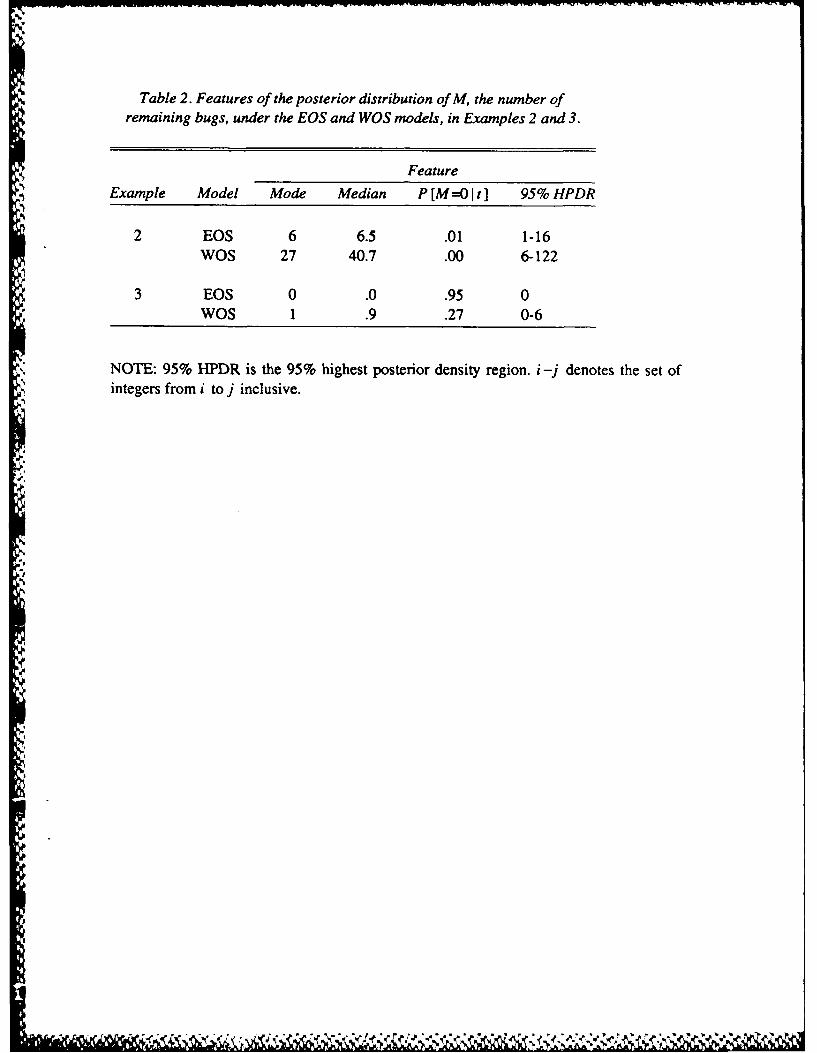
Table 2. Features of the posterior distribution of M, the number ofremaining bugs, under the EOS and WOS models, in Examples 2 and 3.

FeatureExample Model Mode Median P [M=O It] 95% HPDR

2 EOS 6 6.5 .01 1-16WOS 27 40.7 .00 6-122

3 EOS 0 .0 .95 0WOS 1 .9 .27 0-6

NOTE: 95% HPDR is the 95% highest posterior density region. i -j denotes the set ofintegers from i to j inclusive.

9

Captions for Figures I and 2:

Figure 1. Posterior distributions of M, the number of remaining bugs, in Example 2 under (a)

the EQS model, and (b) the WOS model. The WOS model, which is favored by the data, estimates

a much larger number of remaining bugs than the EOS model.

Figure 2. Posterior distributions of M in Example 3 under (a) the EOS model, and (b) the WOS

model. Under the EOS model, almost the entire posterior distribution of M is concentrated at 0,

while from the WOS model, which is favored by the data, it appears that there may be up to six

remaining bugs with non-negligeable probability.

..

4.!

U, 8

--- --- -- --

Figure 1

N. 0

~-CD

SIi , ..................................................... ............ ......... ..........................................

0 20 40 60 80 100 120 140

M(a)

!0

11 1 1 1 i I I It I I I III. . .

0 20 40 60 80 10O0 120 140

(b)

Figure 2

24 0 1

((a

0

CLJ

o246 8 10

M(a)

WRp.

.4