Ambiguity in Social Learning

A test of the Multiple Priors hypothesis

Luis Sanchez

A thesis presented for the degree ofBachelor of Arts

Department of Economics

Columbia University

April 2017

This page is intentionally left blank

Ambiguity in Social Learning

A test of the Multiple Priors hypothesis

Luis A. Sanchez

Abstract

Are there differences in learning when information is ambiguous relative to whenit is not? This paper explores how the introduction of ambiguity in a social learninggame affects the strategies chosen by players. We test the multiple priors model in alaboratory experiment of informational cascades. Our findings suggest a high levelof probabilistic sophistication in part of our subjects and provide limited support forthe multiple priors hypothesis. Although a substantial number of subjects exhibitthe traditional ambiguity averse preferences in an independent elicitation task, weconclude that ambiguity has little to no effect in social learning even when werestrict attention to ambiguity averse subjects.

Acknowledgements: While I alone am responsible for this thesis, I am indebted to manypeople for their insightful comments and suggestions. For this reason, I wish to thankthose who have supported me throughout my work on this thesis. First and foremost, Iwish to thank Alessandra Casella, my thesis advisor, for her academic supervision andpersonal support throughout the past couple of years. Without her, this project would notbe at the point of completion nor would I be on my way to a PhD program in economics.I also wish to thank (in alphabetic order) Mark Dean, Judd Kessler, Pietro Ortoleva,and Bernard Salanie, for their insightful comments at various stages of this work, and tothank the participants of the Experimental Luncheon and the Honors Thesis Seminar fortheir feedback in various presentations of this project.

1

1 Introduction

Everyday there are situations in which individuals have to make inferences about the

world under uncertainty with the opportunity to learn from private (only available to

the individual) and public (available to all individuals) information. This situation, often

termed ”social learning”, has been explored in the literature in scenarios where agents face

well-defined risks. However, because there are different types of uncertainty, individuals

may have difficulties summarizing uncertainty into well-defined risks in ways that may

affect their behavior.

Social learning has been studied under various names such as informational cascades

(Banerjee 1992; Bikhchandani et al. 1992), herding behavior (Celen and Kariv 2004),

tipping-point models (Granovetter 1978; Miller and Page 2004), among others. Early

theoretical developments concluded that social learning can produce ”informational cas-

cades”, a form of herding that occurs when decisions are carried out in sequential order

and public information crowds out the private information of subsequent decision-makers

(Bikhchandani et al. 1992; Banerjee 1992). Although this herding behavior is completely

rational, it may lead agents to converge on an incorrect course of action if feedback is not

readily available.

Real-world scenarios of this type are plentiful and the strong predictions of such

models indicate potential for experimental investigation. For example, suppose you are

part of a group of venture capitalists, each of whom, in deciding whether to invest or

not in a firm, acquires a noisy but informative signal about the prospects of the firm.

Suppose your private signal suggests that the firm will yield a profit and that you should

invest. However, you observe other firms declining to invest. Intuitively, it is obvious that

there is information in what others are doing even if you do not know what information

they hold. This sort of problem has been studied both in the laboratory and in the field.

Yet, all experiments we are aware of have relied on the assumption that probabilities over

states are well-defined.

2

In this paper, we define ambiguity as uncertainty about probabilities over states.

Notice that this definition is rather broad, a point to which we return in the next section.

Our motivation for this project stems from a large body of research suggesting that

individuals treat choices with precise probabilities differently from those with ambiguous

probabilities (Ellsberg 1961; Camerer and Weber 1992; Ivanov 2011; Kelsey and LeRoux

2015; Moreno and Rosokha 2015).

Although a plethora of approaches have been developed to accommodate differences

in decision-making under risk and ambiguity, we focus on a particular model of choice that

suggests that, in the presence of ambiguity, agents form a set of multiple priors - rather

than a unique one - over which they calculate a set of posterior beliefs. Then, using

an exogenously-determined decision-rule, they choose among one of their prior beliefs

(with the corresponding posterior) and act accordingly (Schmeidler 1989; Machina and

Siniscalchi 2014). In order to explore the multiple priors hypothesis in individual and

social learning, we adapt the informational cascades experiment of Anderson and Holt

(1997) and show that, in the symmetric case, ambiguity over the precision of the private

signals is non-instrumental. In other words, the absence of this information should not

impact the strategy an agent chooses. On the other hand, other sources of ambiguity, such

as beliefs about other players’ rationality, should matter depending on what prior belief is

incorporated during choice. This leads to a natural experiment design: under the multiple

priors, any ignorance over the exact precision of the signal should not affect behavior in

an individual learning or social learning setup; but ignorance over the rationality of others

should affect behavior in the social learning game.

Our findings suggest that the subjects in our sample are particularly sophisticated

given their performance in the games. Overall, we find that subjects play according to

Bayes rule in over 80% of all trials. An independent test of ambiguity preference, which

resembles the traditional task used in the Ellsberg Paradox, finds that a majority of

subjects are ambiguity neutral (about 50%) and ambiguity averse (about 35%). However,

3

we find limited support for the multiple priors model in social learning. Our first test,

which tries to determine whether a subject’s strategy differs based on whether subjects

know the precision of the private signals, is unable to reject the multiple priors model.

We note, however, that this test can only reject the model but cannot distinguish it

from other theories such as expected utility theory. Our second test, which seeks to test

whether there is evidence of the ”worst prior” regarding beliefs of other’s rationality in

the social learning game, fails to provide evidence that subjects behave according to the

multiple priors model. To provide a sharper test of this last hypothesis, we separate

subjects according to ambiguity preference and repeat our second test. Despite the

substantial heterogeneity in ambiguity preference across subjects, we are unable to find

support for the multiple priors hypothesis even when we restrict attention to ambiguity

averse subjects.

We divide the rest of the paper in the following manner: In Section 2 we review the

relevant literature on decision-making under ambiguity and social learning. In Section 3

we introduce the model and the predictions we seek to test with our experiment. Section

4 details the experimental design and Section 5 follows with the analysis of our results.

Section 6 concludes. Lastly, Appendix A contains additional proofs omitted in the main

text and Appendix B contains additional graphs omitted in the main text. Appendix

C includes copies of the experimental instructions and screenshots of the computerized

experimental platform.

2 Literature Review

The inspiration for this experiment stems from real-world environments in which both

private and public information are available and thus social learning is possible. Since

information about the underlying probabilities is often incomplete, we focus on reviewing

the literature on ambiguity and social learning and situate our paper within this larger

4

framework.

2.1 Ambiguity in Decision-Making

First, it is important to mark the distinction between risk and ambiguity1. If an agent

is unsure about which state of the world will occur but knows the probabilities of each

state precisely, this is referred to as risk or unambiguous probability. On the other

hand, ambiguity arises when a person does not know with certainty the distribution of

probabilities over states (Becker and Brownson 1964).

A seminal article by Ellsberg (1961) introduced an elegant paradigm that distin-

guished risk from ambiguity through a set of thought experiments similar to the one

described below. Suppose a subject is presented with an urn containing 30 yellow balls

and 60 red and blue balls in an unknown ratio (as shown in Figure 1). The subject is

asked to make a pair of bets whereby he receives a positive payoff if he wins and otherwise

receives nothing. The first gamble, which corresponds to Situation A in Figure 1, asks

the subject to bet either on a yellow ball or on a red ball. Note that there are exactly

30 yellow balls and there can be anything between 0 to 60 red balls. The second gamble,

Situation B in the figure, asks the subject to bet on either a red ball and a blue ball or on

a yellow ball and a blue ball. Once again, we have one risky option that is well-defined,

i.e., there are 60 balls that are red or blue for sure, and one that is not.

A large body of experimental evidence testing this paradigm finds that people often

prefer the risky prospect over the ambiguous one (Becker and Brownson 1964; Kelsey

and LeRoux 2015). In the case presented above, most subjects bet on the yellow ball in

the first gamble and on the red and blue ball in the second gamble. This result, which

is known as the ”Ellsberg Paradox”, is striking since it implies serious violations of the

probability or the expected utility axioms. For instance, under the independence axiom2

1. Although these definitions have existed in the literature under other names, e.g., ambiguity is alsoknown as Knightian uncertainty (Knight 1921), the one presented here captures the central aspects ofthe most common ones.

2. One can also see that the sure-thing principle, the analog of independence under subjective expected

5

Figure 1: Illustration of the Ellsberg Paradox.

of expected utility theory, if subjects prefer a gamble on yellow over a gamble on red,

as shown in Situation A in Figure 1, they must also prefer a mixture of gambles on

yellow and blue over a mixture of gambles on red and blue, contrary to what is shown in

Situation B in Figure 1. An alternate interpretation is that the probability axioms are

violated, thus rejecting probabilistic sophistication in part of the agent. For example, it

may be that subjective probabilities are subadditive, i.e., Pr(A) + Pr(B) ≤ Pr(A ∪B).

In this case, the agent may believe that the probability of drawing a yellow ball is greater

than that of drawing a red ball. However, when the blue ball is added to both options, the

probability of a yellow or blue ball is now subjective and thus subadditive. In turn, this

subjective probability of drawing a yellow or blue ball is now smaller than the objective

probability of drawing a red or blue ball.

Since the Ellsberg Paradox was first proposed, a number of theories have been

developed to accommodate this phenomena. Camerer and Weber (1992) write a com-

utility, is violated following a similar line of reasoning.

6

prehensive review of ambiguity aversion and, more generally, of decision-making under

ambiguity. In addition to providing a review of experimental and empirical evidence, they

discuss alternate theories of decision-making that either relax existing axioms or provide

alternate interpretations for the paradox. In their survey, they conclude that ambiguity

7

preferences exhibit individual heterogeneity and domain-specificity. The table3 in the

previous page, labeled Table 3, highlights the breadth of studies that have replicated the

Ellsberg paradox and found support for ambiguity preference along with the sensitivity

of this finding with respect to the decision context, e.g., low vs. high probabilities, gains

and losses, etc.

For example, Curley and Yates (1989) ask subjects to rank menus of two-outcome

lotteries (one outcome being zero and the other some positive amount of money) that in-

volved risk and ambiguity. By varying the lotteries in probability and monetary rewards,

they find that subjects are willing to pay a premium of up to 10% of the expected value

of a gamble to avoid ambiguity when the probability of gain in the risky lottery ranged

from 50% to 75%. On the other hand, they find that subjects need to be compensated

approximately the same premium to forgo ambiguity when the probability of gain in the

risky lottery was below 25%. In more recent experiments, Kelsey and LeRoux (2015)

look for evidence of ambiguity preference in a Battle of the Sexes game and they find

that about 50% of subjects exhibit the traditional ambiguity-averse preferences - a result

that is comparable to that of previous studies. However, in an experiment that classified

subjects along ambiguity preference, risk preference, and strategic sophistication in a

normal-form game, Ivanov (2011) finds that 32% of subjects are ambiguity loving, 46%

are ambiguity neutral, and the rest are ambiguity averse. Compared to other studies, the

results of Ivanov (2011) differ from past experiments in the small proportion of ambigu-

ity averse subject in their sample. This finding provides some evidence for the notion

that there is substantial individual heterogeneity in ambiguity preference across decision

domains.

3. Table 3 from Camerer and Weber. 1992. ”Recent developments in modeling preferences: Un-certainty and ambiguity” in the Journal of Risk and Uncertainty. Volume 5, issue 4. Obtained andreproduced with permission of Springer.

8

2.1.1 Ambiguity Aversion: Theoretical Approaches

In the absence of information regarding the likelihood of an outcome, a normative re-

sponse is to presume all outcomes to be equally probable (Laplace’s Principle of Insuffi-

cient Reason). However, this principle is inconsistent with the behavior observed in the

Ellsberg paradox. One theoretical approach to explain the preference of risky gambles

over ambiguous ones has been to use second-order probabilities. A second-order prob-

ability refers to a probability function that describes the likelihood that another set of

probabilities (the first-order probabilities) describe the states of the world. Thus, in the

case of the Ellsberg paradox, each first order probability refers to a specific distribution

of the contents of the urn and the second order probability refers to the likelihood of each

of these distributions. This formulation should be reminiscent of a compound lottery

and, for the expected utility maximizer, this is resolved by reduction of compound lot-

teries. To resolve the inconsistency between expected utility and the Ellsberg Paradox,

Ergin and Gul (2009) relax the reduction of compound lotteries axiom, such that the

agent does not reduce compound lotteries to the simple lottery equivalent, and reinter-

pret ambiguity as second order risk aversion (analogous to the standard notion of risk

aversion based on mean preserving spreads). From a normative perspective, this theory

is attractive and capable of explaining the paradox given some mild assumptions about

how the composition of the ambiguous urn is determined.

The approach of Ergin and Gul (2009) was preceded by Becker and Brownson

(1964) who define ambiguity as ’any distribution of [second order] probabilities other

than a point estimate’ and operationalize ambiguity aversion as a measure increasing on

the range of the second order probabilities. In this sense, an agent would prefer a gamble

with a second order probability defined by a point estimate to one defined by any non-

degenerate second-order distribution - thus providing a solution to the Ellsberg paradox.

In an experiment that offered subjects a choice between gambles with the same expected

value but with varying second order distributions (from a point estimate to a uniform

9

distribution over the entire domain), Becker and Brownson (1964) find that subjects are

willing to pay increasing amounts to avoid gambles with larger spreads of the second

order distributions.

In a related test of this hypothesis, Yates and Zukowski (1976) ran an experiment

in which subjects are asked to rank and price three gambles. Each gamble corresponds

to one of three urns containing 10 chips each: a ”risky urn” containing 5 red chips and 5

blue chips; a ”uniform urn” with the number of red chips determined using a uniform dis-

tribution between 0 to 10 (with the balance, if any, being blue chips); and an ”ambiguous

urn” in which subjects have no information about the underlying probabilities used to

determine the composition of the urn. If the second-order probability hypothesis holds,

the risky urn is strictly preferred to the uniform urn and weakly preferred to the ambigu-

ous urn (as the second order probability may be a point estimate). Furthermore, since

the uniform urn represents the maximal spread, the ambiguous urn should be preferred

to the uniform urn. Consistent with this hypothesis, subjects were willing to pay an av-

erage premium of 20% of expected value to bet on the risky urn instead of the ambiguous

urn. However, they also find that the ambiguous urn was the least-preferred and lowest-

priced of all three. Thus, their experiment provides evidence against the hypothesis that

second-order probabilities fully resolve the Ellsberg paradox.

Other approaches include attempts to relax the probability axioms or find other

alternatives to expected utility theory. Segal (1987) adopts the assumption that ambigu-

ity can be expressed as a second-order distribution that is not decomposed in the same

way a compound lottery would be under expected utility. Then, using the anticipated

expected utility model, he is able to reconcile the paradox. Similarly, Schmeidler (1989)

introduces non-additive probabilities (also called a capacity), i.e., Pr(A) + Pr(B) 6= Pr(A

or B), to create a generalization of subjective expected utility theory. To accomplish this,

Schmeidler axiomatizes the use of the Choquet integral4 in evaluating acts. The intuition

4. In general, when the Choquet integral is defined over a capacity h that is not a probability measure,it has the property of being non-additive, i.e., given some functions f and g,

∫fdh+

∫gdh 6=

∫(f+g)dh.

10

is as follows: first, the agent ranks all possible states according to their attractiveness;

then, the utility of an outcome is weighed by the difference in cumulative capacities. Note

that when the capacity is additive then we have probability measure and this second step

is equivalent to the difference in cumulative probabilities, thus collapsing to subjective

expected utility. In turn, this process is able to accommodate the Ellsberg paradox under

ambiguity.

2.1.2 Multiple Priors

Only a few of many approaches to ambiguity aversion and the Ellsberg paradox have been

explored in the previous section. Since the experiment presented in this paper builds on

the theory of multiple priors, we devote a section to this paradigm.

The multiple priors approach supposes that the Ellsberg paradox can be explained

by a more general criterion that combines Bayesian and maximin5 principles (Zappia

2015). Gilboa and Schmeidler (1989) propose a Maximin Expected Utility (MEU) model

which relaxes the independence axiom6 of expected utility and replaces it two other ax-

ioms: Uncertainty Aversion and Certainty Independence. The former reflects a preference

for hedging while the latter ensure that constant prizes do not provide hedging. In addi-

tion, it presumes that, under ambiguity, an agent possesses multiple priors over which he

or she forms posterior beliefs and calculates expected utilities. Then, the agent uses the

maximin principle to choose from this set of priors (with the corresponding posterior) as

if trying to maximize the minimum expected payoff (i.e., as if Nature is playing against

him or her when choosing an action).

First, note that there are multiple sets of non-unique priors that result in Ellsberg-

type behavior. The model assumes the space of priors is exogenously determined. Second,

similar to previous theories, the multiple priors model has a normative flavor because the

5. The maximin principle refers to the idea that the agent behaves as if they are maximizing theminimum possible expected payoff rather than maximizing expected utility.

6. Independence implies the sure thing principle of subjective expected utility. Since the Ellsbergparadox directly contradicts the sure thing principle, then independence must be violated.

11

agent is Bayesian and the problem has a structure that resembles a compound lottery.

However, the model provides flexibility in terms of the decision criterion used to choose

from the set of prior beliefs available to the agent. It should be obvious that this model can

favor different courses of action depending on the set of priors. More generally, however,

the agent does not need to choose the worse possible posterior. Other models have

adopted the multiple priors approach with other criteria such as a mixture of maximin

and minimax principles (Machina and Siniscalchi 2014).

2.1.3 Ambiguity Aversion in Non-Comparative Contexts

Our main experiment differs from past studies of ambiguity aversion in that subjects are

not presented with a comparative choice, i.e., a choice between an ambiguous and unam-

biguous prospect. The ambiguity aversion we are interested in arises out of insufficient

information in the decision context. This is an important distinction and a source of

concern because there is conflicting evidence as to whether ambiguity aversion persists

when the decision-maker does not face a comparative choice.

For instance, the ”competence hypothesis” (Heath and Tversky 1991) suggests that

behavioral differences, in terms of preferring either the risky or the ambiguous prospect,

are determined by how competent the agent feels to make the right choice. In a set of

studies, Heath and Tversky (1991) present subjects with a choice between a lottery and

an ambiguous bet, both of which are in a domain in which the subject felt competent,

e.g., politics or sports, and find evidence of ambiguity aversion. However, when they

repeated the same task in a domain in which the subject felt incompetent, the effect

disappeared. In a related line of thought, the ”comparative ignorance hypothesis” (Fox

and Tversky 1995) suggests that ambiguity aversion results when both an ambiguous

and a risky gamble are jointly evaluated because the subject feels more competent with

the risky gamble relative to the ambiguous one. In turn, their hypothesis also predicts

that ambiguity aversion diminishes if an ambiguous bet is evaluated in isolation (Fox and

12

Tversky 1995).

Other researchers have revisited the comparative hypothesis and found that, al-

though the effects of ambiguity aversion are stronger in comparative contexts, earlier

claims that the effects vanish in non-comparative problems are much more fragile than

previously thought (Chow and Sarin 2001; Fox and Weber 2002). In an experiment, Fox

and Weber (2002) find that ambiguity-aversion can be elicited in non-comparative con-

texts and strategic games as long as ambiguity is salient. Along the same lines, Kelsey and

LeRoux (2015) develop an experiment to determine the influence of ambiguity in strat-

egy selection in a Battle of the Sexes game in which the column player has an additional

”ambiguity-safe” action (in addition to the traditional two coordination options) that is

not part of any equilibrium strategy. Their results show that even when the ambiguity-

safe option is dominated by randomizing with respect to the coordination strategies, a

third of subjects still choose this off-equilibrium move. As expected, increasing the payoff

of the ambiguity-safe option also increases the column player’s propensity to choose it.

2.1.4 Individual Learning Under Ambiguity

The experiment described in this paper tests the implications of the multiple priors

model in a social learning and individual learning task. In this section we describe some

results from the literature on individual learning under ambiguity7. Two central questions

explored in the literature on learning are whether subjects use the information they are

given and whether they update their beliefs according to Bayes’ Rule.

First, research suggests that subjects heavily discount ambiguous information in

decisions that involve simple choices with incomplete and conflicting information about

costs and benefits. In an experiment, Dijk and Zeelenberg (2003) asked subjects to

make investment decisions in a hypothetical scenario that either involved clear informa-

tion, conflicting information, or no information regarding the cost of the project. Those

7. For a more comprehensive review of learning under ambiguity, see Epstein and Schneider (2007).

13

who received no information or received conflicting information about the cost were 30%

likely to continue the project while those who received clear information were 60% likely

to continue it. In a follow up experiment, they tested a similar paradigm with informa-

tion about the probability of success of an investment project. Similar to their previous

results, 31% and 25% chose to continue the project (difference is not significant) in the

no information and conflicting information treatments, respectively. Yet, this proportion

rose to over 55% when exact probability estimates were given. The results of this exper-

iment suggest that ambiguous information, defined as missing or conflicting information,

is treated differently from well-defined information (at least in hypothetical investment

decisions).

Similarly, in an experiment that is closer to the one we present in this paper,

Trautmann and Zeckhauser (2013) asked subjects to bet, by choosing a color, on one

of two bags: a bag with 5 red and 5 black poker chips or a bag with 10 black or red

chips but in an unknown composition. Once a subject chose a bag and a color, the

experimenter drew a chip, which was visible to the subject, and then put it back in the

bag. Immediate after, the subject was asked again to bet on a color to be drawn from

the same bag. This procedure is known to the subject before the task begins and thus

the ambiguous gamble offers the agent the possibility of learning because the first draw is

statistically informative of the contents of the bag. Their results suggest that subjects did

not understand that learning was possible in these games and often shunned the learning

possibility offered by the ambiguous prospect even though it provided a premium over

the risky prospect.

In another experiment, which tries to answer whether subjects update according to

Bayes’ Rule, finds that individuals significantly overweigh new information under ambi-

guity (and thus update incorrectly) despite performing very well when faced with learning

under risk (Moreno and Rosokha 2015). In this paper, subjects were asked to make bets

on two urns, one risky and one ambiguous, containing four black or white balls: the

14

risky urn has one, two, or three black balls while the ambiguous urn has one black ball,

one while ball, and two balls of either color (but the color of these last two balls is not

revealed to the subject). This information was known to all subjects before they were

asked to make a bet. To determine the impact of ambiguity in individual learning, each

subject observed a sequence of draws (with replacement) and then completed a multiple

price list in which he chose between a sure payoff and a bet on one of the urns. Subjects

received a total of twelve draws from each urn and were asked to complete the multiple

price list after every three draws. Using a statistical model, the authors conclude that

participants use a prior that is inconsistent with the Principle of Insufficient Reason,

i.e., in the absence of information that one outcome is more likely than another all out-

comes are treated as equally probable, which corresponds to an urn with two white and

two black balls for the ambiguous urn. Furthermore, their model suggests that subjects

overweighed each new signal in the ambiguity treatment but not when faced with risk.

2.2 Social Learning

We now proceed to summarize the literature on social learning. Although this area has

been studied extensively, there are no papers, to our knowledge, that have investigated

the relationship between ambiguity and social learning. We devote a significant amount

of time to the informational cascades model because the experiment presented later is

based on it.

Banerjee (1992) and Bikhchandani et al. (1992) present two versions of the classical

informational cascades model, differing only on how ties are decided. This model describes

situations in which agents receive an informative signal about the current state of the

world and are tasked with choosing from a finite set of actions. The social aspect is

introduced because individuals are allowed to learn from the actions that others have

taken, conditional on their private information.

Agents are arranged in an exogenously-determined sequence and each is given a

15

conditionally independent signal along with the history of past decisions. Each agent is

then asked to make an inference about the current state of the world. The model predicts

that a pure Bayesian equilibrium exists in which, after a certain point, it is optimal for all

agents to go against their their private information if it contradicts the cascade. Thus,

choices become imitative and are uninformative to subsequent decision-makers. This

result is known as an ”informational cascade”. Banerjee (1992) and Bikhchandani et

al. (1992) derive other predictions from their model. First, cascades form asymptotically

with probability one and the speed with which these forms depends on the precision of

the signals. Second, cascades are not fragile under Bayesian updating. In other words, if

all agents are rational and Bayesian, then the chance of a cascade breaking is zero.

Celen and Kariv (2004) provide a discussion and an experimental design that dis-

tinguishes between an informational cascade and a herd. They argue that, in the former,

agents settle on a pattern of behavior in which the absence of their private signal does

not impact their choice and thus the pattern of behavior is stable. On the other hand,

herd behavior is characterized by agents settling on a pattern of behavior in which they

are more likely to imitate the actions of the herd but private signals can still provide

provide information. Thus, herd behavior is fragile to strong signals. Their discussion is

in line with the other experiments that try to distinguish between conformity and social

learning (Goeree and Yariv 2015).

Anderson and Holt (1997) test the informational cascades model in a set of exper-

iments in which subjects are presented with one of two urns, Urn A or Urn B, chosen

using a fair coin before the round begins. Although subjects are aware of how the urn

is chosen, they do not know which one is selected. Urn A contains two balls labeled ”a”

and one ball labeled ”b”, while Urn B contains two balls labeled ”b” and one ball labeled

”a”. The most important aspect of this set up is that any draw from the urn will be

statistically informative about which urn it comes from. Individuals then use their condi-

tionally independent signal (their ”private” information), along with the history of past

16

choices, (the ”public” information8), to make an inference about what urn was chosen

for the round.

Their results suggest that, for the most part, people’s decisions were consistent with

Bayesian updating which implies that they ignored their private information if Bayes’

Rule dictated a course of action inconsistent with their private signals. Nevertheless, in

26% of all cases, when the optimal Bayesian decision was inconsistent with a decision

based only on private information, players chose to follow their own private information.9

The authors test a variety of behavioral theories, i.e., status quo bias and the represen-

tativeness heuristic, but do not find sufficient information to support any of these biases

as the driver of the results. However, they also conclude that their experimental results

suggest that it is unlikely that informational cascades develop as proposed by the model

since these appear to be fragile to individual deviations from Bayesian updating. This last

point deserves further elaboration since, if common knowledge of rationality is relaxed

and agents are allowed to question other players’ rationality, some apparent deviations

are rational (e.g., the case where a player ignores the history because he or she believes

others choose an action randomly).

Goeree et al. (2007) investigate the formation and collapse cycles of informational

cascades using longer sequences, 20 or 40 participants, in a experiment similar to An-

derson and Holt (1997). In different treatments, they vary the precision of the signal

between the urns such that either 5 or 6 balls out of a total of 9 match the urn’s color.

Their results show that cascades often break (more than 85% of the time across all condi-

tions) and even reverse. The main contribution of this paper, however, is the application

to social learning of the logit Quantal Response Equilibrium (logit QRE) model, which

allows agents to deviate and to account for others’ deviations from the optimal Bayesian

8. In three sessions, the public information also included a ”public draw” from the urn.9. Individuals generally used information efficiently and followed the decisions of others when it was

rational. There were, however, some errors, which tended to make subjects rely more on their ownprivate information, as indicated by a logit model with decision errors. The most prevalent systematicbias is the tendency, for about a third of the subjects, to rely on simple counts of signals rather thanBayes’ rule.

17

updating strategy. QRE stipulates that the probability with which an action is chosen

is a smooth increasing function of the expected payoff from that action, relative to other

available actions. One central feature of the QRE model is that it incorporates a rational-

ity parameter, λ, which parametrizes the sensitivity to differential payoff gains and may

potentially differ across subjects. The authors combine the logit QRE model with other

behavioral models as in Anderson and Holt (1997). They find that the best fit for the

observed data is a QRE model combined with a cognitive hierarchy model, which allows

for multiple degrees of sophistication among players, and a base-rate fallacy model, in

which agents overweight their private information relative to public information.

In a different design, Celen and Kariv (2004) opt for a continuous signal setup and

try to distinguish informational cascades from herd behavior. In their experiment, a total

of eight agents are arranged in a sequence and each one is endowed with a private signal

drawn from a uniform distribution of values within the interval [-10,10]. Based on the

private signal, each agent has to choose either action A or action B where action A is

profitable if the sum of all private signals is positive and action B is profitable if the sum

is negative. Unlike the binary informational cascades setup, where cascades cannot be

reversed if agents are Bayesian, the continuum design allows for deviations to be infor-

mative because future agents can conclude that the deviator has private information that

is so convincing that it leads him/her to deviate. The longer the sequence of individuals

who choose A, the harder it is for a single individual to choose action B, and thus a

deviation is very informative to future agents. The authors find that herd behavior (of

at least five subjects) was observed in 27 of the 75 rounds with all but one herd in the

correct direction. Using a recursive model to determine how well a Bayesian framework

can explain their results, they conclude that agents earlier in the sequence weigh their

own signals too heavily and give too little weight to public information. Since later agents

appear more Bayesian, the authors hypothesize this result may be consistent with beliefs

in which other agents tremble when making decisions.

18

Our setup, discussed in the next section, presents a case in which priors about the

precision of the signal have no impact on behavior but beliefs about other’s rationality

do. This design allows us to reject the multiple priors model through two distinct mech-

anisms. Because no prior on the precision of the signal should affect behavior if subjects

make choices when informed or not informed of such precision, the differences cannot be

explained via the multiple priors model. However, social learning introduces an additional

source of ambiguity stemming from uncertainty about the rationality of others. In the

absence of common knowledge of rationality, the multiple priors model predicts different

behavior from that of the standard expected utility model. To determine whether the

deviations arise from the ambiguity over other’s rationality, we compare an informational

cascade model in which social learning is possible and one in which the social aspect is

absent.

3 The Model

In this section we provide a model of social learning similar to the Bikhchandani et

al. (1992) and Banerjee (1992). We focus exclusively on the symmetric case and adapt

the notation to fit the context of our experiment.

3.1 General Structure

Let P = 1, ..., N be a set of subjects arranged in a sequence such that i ∈ P is the

ith subject to make a choice ci ∈ C = R,B where R corresponds to a guess in favor

of a RED urn and B corresponds to a guess in favor a BLUE urn. All subjects have a

common prior for the payoff relevant state space Ω = R,B in which R and B stand

for a RED or BLUE urn, respectively, being chosen by Nature with Pr(R) = Pr(B) = .5

before the subjects begin their play10.

10. The uniform prior is a feature of the symmetric game. In addition to making the game moreintuitive and easier to solve, it is necessary for the theorem proved in the next section.

19

Each agent i receives a conditionally independent signal si ∈ S = r, b, where r

stands for a red ball and b stands for a blue ball in our experiment, with probabilities

Pr(b|B) = Pr(r|R) = p > .5 and Pr(r|B) = Pr(b|R) = q such that q = 1 − p. In our

experiment, both urns contain balls that are either blue or red in color with the restriction

that a majority of balls match the color of the urn (as dictated by p). Our assumptions

about the signals imply that the conditional probability of drawing a ball of a color that

matches the color of the urn is the same for both urns and that this draw is statistically

informative of the state chosen by Nature. It is common knowledge that p > .5.

Denote the history of choices observed by agent i as Hci = (cj)j<i : j ∈ P, ci ∈ C

if i > 1 and Hci = ∅ otherwise. Similarly, let Hs

i = (sj)j<i : j ∈ P, si ∈ S denote the

history of past draws up to agent i if i > 1 or Hsi = ∅ otherwise. Notice that if agents

observe the history of signals, Hsi , the set-up is equivalent to an individual learning game.

Instead, if they observe the history of choices, Hci , the set-up is a social learning game.

The game that subjects play, either the social learning or individual learning game, and

thus which history11 is common knowledge to all subjects.

Subjects receive state-dependent payoffs based on their choice ci, with a correct

guess of the state being rewarded with some positive payoff and an incorrect guess with

a payoff of zero. We normalize the utility of the positive payoff to one and the utility of

receiving nothing to zero. Since an agent’s payoff is not affected directly by the actions

of others, then the utility of agent i is a mapping Ui : C × Ω→ 0, 1.

3.2 Equilibrium

Denote the profile of behavioral strategies for the game by σ = (σ1, ..., σN), where σi, the

strategy of player i, is the probability of choosing ci = R, with σi : Si ×Hi → ∆(C) for

any history observed by the agent. Similarly, let γi be the posterior belief of subject i

that the state chosen by Nature is RED conditional on the information available to the

11. To simplify the use of notation, Hi is used without a superscript in cases where it applies to boththe history of signal or the history of choices.

20

subject. Thus, we define the mapping γi : Si × Hi → [0, 1] for any history observed by

the agent.

In turn, we can use this notation to define agent i’s expected utility over actions

(taking into account the normalized utility of the payoffs) as follows.

EUi(ci, si, Hi) =

γi, if ci = R

(1− γi), if ci = B

Since we assume that agent i is rational, he maximizes his expected utility over his

set of actions and chooses the optimal strategy. Given the history and his own signal, the

agent determines his posterior beliefs over states using Bayes’ Rule. Then, his behavioral

strategy over actions takes the following form:

σi(si, Hi) =

1, if γi > .5

0, if γi < .5

Because the expected utility over actions and the strategy of the agent depend solely

on the posterior beliefs, we can define a Perfect Bayesian Nash Equilibrium (PBNE) of

the game as the profile of strategies σ and the corresponding system of posterior beliefs

γ such that for any agent i,

σi ∈ argmaxci

EUi(ci, si,Hi)

Note that the strategy is left unspecified for the case when the subject’s beliefs do

not clearly favor a course of action. This knife-edge case, when the agent is indifferent

over states, γi = 1 − γi, is determined according to a tie-break rule that is common

knowledge. For example, some natural candidates for breaking ties are the ”confident”

tie-break rule, in which the subject chooses to call his own private draw when indifferent

(similar to the rule used by Anderson and Holt 1997), or a ”coin-flip” rule in which the

21

subject determines his choice using a randomization device.

If the tie-breaking rule is the same for all subjects in the game, as assumed by

Bikhchandani et al. (1992) and Banerjee (1992), the eventual formation of an ”informa-

tional cascade”12 is the unique PBNE of this game. Uniqueness of the solution can be

established by eliminating dominated actions at each node in the game tree. Notice that

the tie-break rule allows us pin down the equilibrium by eliminating an action when the

strategy fails to establish a unique action. One last point worth emphasizing is that the

tie-break rule need not be the same for all subjects for the results introduced in the next

section. However, the assumption that the tie-break rule is the same across subjects is

crucial in terms of pinning down the equilibrium. Koessler and Ziegelmeyer (2000) prove

that there always exist a set of tie-break rules that rationalize any observed history of

actions in equilibrium.

3.3 Non-Instrumental Information

We define information as non-instrumental if the profile of equilibrium strategies of a

game remains unchanged regardless of what beliefs agents hold about this information.

Theorem 1. The value of p, which indicates the precision of the private signal, is non-

instrumental as long as p > .5.

The proof of the theorem is in two parts; first we show this holds when agents

observe the history of signals and then proceed to show it holds if they observe the

history of choices. We prove that the subject’s strategy, which hinges on their posterior

beliefs, is not affected by precise knowledge of p (as long as it is commonly known that

p > .5). This, in turn, implies that the profile of equilibrium strategies of the game does

not change.

12. Following the definition provided by Bikhchandani et al. (1992), ”an informational cascade occurswhen it is optimal for an individual, having observed the actions of those ahead of him, to follow thebehavior of the preceding individual without regard to his own information”.

22

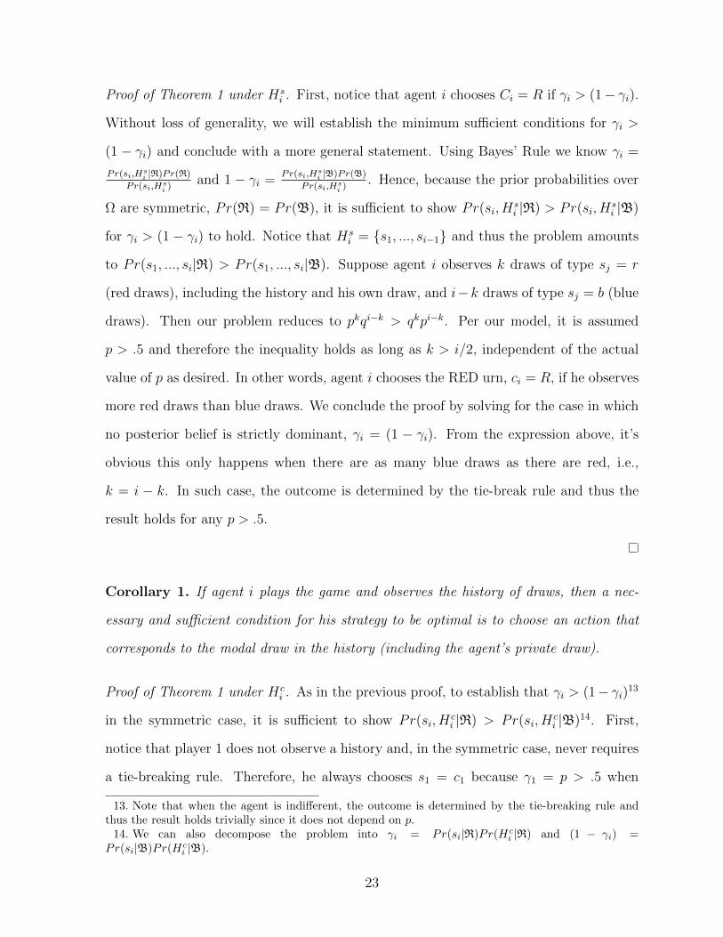
Proof of Theorem 1 under Hsi . First, notice that agent i chooses Ci = R if γi > (1− γi).

Without loss of generality, we will establish the minimum sufficient conditions for γi >

(1 − γi) and conclude with a more general statement. Using Bayes’ Rule we know γi =

Pr(si,Hsi |R)Pr(R)

Pr(si,Hsi )

and 1 − γi =Pr(si,H

si |B)Pr(B)

Pr(si,Hsi )

. Hence, because the prior probabilities over

Ω are symmetric, Pr(R) = Pr(B), it is sufficient to show Pr(si, Hsi |R) > Pr(si, H

si |B)

for γi > (1− γi) to hold. Notice that Hsi = s1, ..., si−1 and thus the problem amounts

to Pr(s1, ..., si|R) > Pr(s1, ..., si|B). Suppose agent i observes k draws of type sj = r

(red draws), including the history and his own draw, and i−k draws of type sj = b (blue

draws). Then our problem reduces to pkqi−k > qkpi−k. Per our model, it is assumed

p > .5 and therefore the inequality holds as long as k > i/2, independent of the actual

value of p as desired. In other words, agent i chooses the RED urn, ci = R, if he observes

more red draws than blue draws. We conclude the proof by solving for the case in which

no posterior belief is strictly dominant, γi = (1 − γi). From the expression above, it’s

obvious this only happens when there are as many blue draws as there are red, i.e.,

k = i − k. In such case, the outcome is determined by the tie-break rule and thus the

result holds for any p > .5.

Corollary 1. If agent i plays the game and observes the history of draws, then a nec-

essary and sufficient condition for his strategy to be optimal is to choose an action that

corresponds to the modal draw in the history (including the agent’s private draw).

Proof of Theorem 1 under Hci . As in the previous proof, to establish that γi > (1− γi)13

in the symmetric case, it is sufficient to show Pr(si, Hci |R) > Pr(si, H

ci |B)14. First,

notice that player 1 does not observe a history and, in the symmetric case, never requires

a tie-breaking rule. Therefore, he always chooses s1 = c1 because γ1 = p > .5 when

13. Note that when the agent is indifferent, the outcome is determined by the tie-breaking rule andthus the result holds trivially since it does not depend on p.

14. We can also decompose the problem into γi = Pr(si|R)Pr(Hci |R) and (1 − γi) =

Pr(si|B)Pr(Hci |B).

23

s1 = r and γ1 = q < .5 when s1 = b. Without loss of generality, suppose that s1 = r and

thus c1 = R.

Since subsequent players observe the history of choices, Hci = c1, ..., ci−1, and

not the history of draws, agent i forms beliefs over the probability of observing a given

history conditional on a state. We approach the belief-formation problem of agent i > 1

under the ”confident” tie-break rule. Note that we only require that tie-break rule to

be common knowledge. Appendix A contains additional proofs for the non-confident,

mixed-confidence, and mixed-color tie-break rules.

Suppose all subjects are endowed with the confident tie-break rule such that, if

agent i faces a tie, he chooses according to his signal, i.e., given γi = 1− γi if si = r then

ci = R and otherwise if si = b then ci = B. In other words, the choice of the agent is fully

informative of his private draw in case of a tie. Since Hc2 = R, player 2, knowing that

player 1 chooses according to his signal, concludes Pr(Hc2|R) = p and Pr(Hc

2|B) = q.

Therefore, player 2 incorporates his private draw and his choice reduces to γ2 = p2 and

1−γ2 = q2 if he receives s2 = r and to γ2 = 1−γ2 = pq if s2 = b. Note that in the former,

player 2 chooses c2 = R, while in the latter, when there is a tie, he chooses c2 = B as a

result of the tie-break rule.

Now consider the choice of Player 3. If the history is Hc3 = R,R, he concludes

Pr(Hc3|R) = p2 and Pr(Hc

3|B) = q2 because he knows player 1 always goes with his

signal and, based on the history, player 2’s action is fully informative of his draw. If

player 3’s draw is s3 = r, his choice reduces to γ3 = p3 and 1 − γ3 = q3. Otherwise,

if s3 = b, it reduces to γ3 = qp2 and 1 − γ3 = pq2. In either case, his posterior beliefs

are γ3 > 1 − γ3 and thus c3 = R independent of his private draw. This is the start of

an informational cascade and all future agents will also choose R independent of their

private information. Thus the result holds true for all future agents in the sequence.

However, if player 3 observes Hc3 = R,B, he concludes Pr(Hc

3|R) = Pr(Hc3|B) =

pq. Because we can decompose the problem into γi = Pr(si|R)Pr(Hci |R) and (1− γi) =

24

Pr(si|B)Pr(Hci |B), it is evident that Pr(Hc

3|R) and Pr(Hc3|B) cancel out and the agent

is left with the same choice as player 1. If his draw is s3 = r, his choice reduces to γ3 = p2q

and 1 − γ3 = q2p; otherwise, if s3 = b, it reduces to γ3 = pq2 and 1 − γ3 = p2q. One

way to understand this result is that because the tie-break rule is perfectly informative

of the agent’s signal, the pair of observed choices ’cancel’ each other out, leaving the final

choice to the agent’s draw.

To show that this concludes the proof, notice that we can decompose any sequence

of actions in the history as described above. If the first two elements are the same, then

we are in a cascade and the result holds. Otherwise, if these elements are distinct, then

these are fully informative and cancel out. Suppose the history has an even number of

elements; then we can proceed to examine the next pair in the same way. For example, for

the histories R,B,B,R and R,B,R,B the first two elements cancel out and so does

the second pair. Therefore, the fifth agent observing these sequences acts as if he was

player 1. On the other hand, for the history R,B,R,R, we can cancel out the first pair

and, upon examination of the second pair, we conclude we are now in an informational

cascade. Instead, if the history contains an odd number of elements, we can use the

same procedure to eliminate all but the last action if each pair contains alternating

elements or to conclude that we are in an informational cascade. If we conclude that

an informational cascade has not begun, then the agent observing the odd sequence of

actions is faced with a choice that decomposes into that of player 2. This concludes the

proof for this tie-breaking rule because the inequalities between γi and (1− γi) are never

reversed as long as p > .5 and thus p is non-instrumental.

3.4 Probability of a cascade occurring

A notable result of the informational cascade model is that the probability of a cascade

occurring is asymptotically one. For instance, if all subjects break ties by reporting

25

the action of their predecessor (non-confident rule in Appendix A), it is obvious that a

cascade will always form since all subjects will report the same action as that of the first

agent.

Similarly, we can consider the probability of a cascade forming under the confident

tie-break rule. Although the result extends easily to an odd number of agents, for illus-

tration purposes, suppose there are N agents in the sequence such that N is even. In

Theorem 1 we concluded that if the history of choices is observed, we can decompose it

by analyzing each pair (e.g. choices by agents 1 and 2, then that of agents 3 and 4, and

so on) starting from the first agent. An informational cascade forms at the first pair with

two similar choices, e.g., in R,B,R,R, ... a cascade forms in the second pair. Thus,

the only sequence that can sustain the absence of a cascade is one in which each pair

has distinct elements. We can express the probability of this event for a sequence of N

agents as follows:

Pr(NoCascade) = (2pq)N/2 = (2p− 2p2)N/2

Two points can be concluded from the expression above. As N gets large, the

probability of the cascade not occurring decreases and it does so rapidly. In turn, the

probability of a cascade occurring is one for N large enough. Second, informational

cascades occur earlier in the sequence as p approaches one and later in the sequence as

p approaches 1/2. To put this numerically, for N = 4 the probability of no cascade

occurring is about 25% when p = .51 and less than .04% when p = .99.

3.5 Instrumental and Non-Instrumental Ambiguity

In Section 3.3 we defined information as ”non-instrumental” if beliefs regarding this

information do not influence the final choice of the decision-maker. In this section, we

bridge the notions of ambiguity and multiple priors with the social learning paradigm.

26

In particular, if p is not known (besides p > .5) and ambiguity aversion is explained by

the multiple priors model then the following proposition ensues.

Proposition 1. Given that p > .5 and this is common knowledge to all subjects, under

the multiple priors model, ambiguity over p does not affect the agent’s strategy.

Recall that under the multiple priors model of ambiguity, the agent forms beliefs

over a set of priors according to Bayes’ rule and chooses between the set of priors according

to some decision rule, e.g. maximin rule as in Gilboa and Schmeidler (1989). Since we

have proven that the precision of the private signals is non-instrumental, then ambiguity

over this piece of information implies that for any set of prior beliefs and any decision-

rule used to select the prior, the choice of the agent is unaffected as long as p > .5 is

commonly known.

Before introducing the experimental design, it is important to underscore the dis-

tinction between the individual learning game and the social learning game. While the

former provides a rather straight forward test of the multiple priors model, the social

learning game introduces new sources of uncertainty that remain undefined and are con-

sequential in determining the strategies that individuals pursue. A new source of ambi-

guity introduced in the social learning game arises from an agent’s beliefs about others’

rationality15. It is worth noting that doubting others’ rationality is not equivalent to

assuming that agents tremble in their choice; however, in our design these two are indis-

tinguishable. The angle we adopt in this paper is that ambiguity over others’ rationality

refers to beliefs about others’ ability to update according to Bayes’ Rule and thus to form

correct beliefs.

For instance, suppose that agents are rational with some probability but the distri-

bution over an agent’s type is unknown. If we consider this problem through the multiple

priors model, the worst possible prior is that others are fully random. Thus, the history

15. Another source of uncertainty is the ambiguity over the tie-breaking rules used by other agents.From the multiple priors perspective, in which agents choose the worst prior, it is unclear what this wouldentail in terms of beliefs or even observed behavior. It remains an open question for future research.

27

Source Observe Choices Observe Signals

Known p Social Learning Individual Learning

Unknown p Social Learning Individual Learning

of choices contains no useful information and should be rationally ignored by the agent.

This result is of particular interest because under the assumption that there is common

knowledge of rationality and that agents are Bayesian, a cascade should never break.

However, previous lab experiments suggest that cascades often break and even reverse

(Anderson and Holt 1997; Goeree et al. 2007) and this may be a result of beliefs over

others’ rationality.

Proposition 2. Under the multiple priors model, equilibrium strategies are not invariant

to ambiguity over other’s types.

In other words, strategies will differ based on the agent’s beliefs of others’ ratio-

nality when their choices, but not their private signals, are observed. Stated differently,

we should expect that behavior across the individual learning game and social learning

game should be different due to ambiguity over others’ types. Particularly, if agents

are accurately described by the multiple priors model with the maximin principle, then

they should ignore the history of actions and solely pay attention to their private signal.

Therefore, one would expect cascades not to form. More broadly, one would expect to see

behavior inconsistent with a social learning game. On the other hand, behavior within

the individual and the social learning games, respectively, should not vary on whether

the agent does or does not know the precision of the private signal so long as p > .5 is

commonly known.

Our two propositions, each corresponding to a source of ambiguity, are summarized

in the table at the top of the page. The rows highlight the that we can introduce ambiguity

over the precision of the signal within the individual learning game and the social learning

game alike. Treatments with the same colors refer to those in which we expect to observe

28

no difference. Thus, as stated before, whether subjects are provided with the precision

of the signal or not should make no difference. The columns emphasize the ambiguity

introduced by the history available to the agents. When subjects observe choices rather

than signals, ambiguity over other’s rationality matters in terms of what strategy is

appropriate. Under the worst prior, we expect to observe differences in behavior across

social and individual learning games, regardless of whether the precision of the signal is

known.

4 Experimental Design

For this experiment sixty students were recruited through the Columbia Experimental

Laboratory in the Social Sciences (C.E.L.S.S) over four sessions - each session with fifteen

subjects. In our sample, 53% of subjects self-identified as female and 70% self-reported

having taking 1 or more probability or statistics courses. In addition, about 52% were

undergraduates, 42% were masters students, and the rest identified as PhD candidates

or other. Participants were informed that the experiment would be in two parts and

that their combined earnings would be paid out in private and in cash at the end of each

session. Both parts of the experiment were programmed using Z-Tree (Fischbacher 2007)

and subjects provided their responses using a computer interface in private cubicles in

the lab. Participants could earn up to twenty-four dollars in addition to a show-up fee of

five dollars. On average subjects earned $23.40 including the show-up fee.

At the beginning of each part, instructions were read aloud to the participants

along with a PowerPoint as a visual aid. The instructions and the visuals used for the

experiment can be found in Appendix C. Before Part I of the experiment, subjects were

required to complete a short quiz to test their understanding of the instructions and

played one practice round. The quiz and screenshots of the experimental interface can

also be found in Appendix C as well. Below, we describe Part I and Part II of the

29

experiment.

4.1 Part I: Individual and Social Learning Task

Part I of the experiment consisted of four tasks: Individual Learning with Risk (ILR),

Individual Learning with Ambiguity (ILA), Social Learning with Risk (SLR), and Social

Learning with Ambiguity (SLA). The distinction made here between risk and ambiguity

refers to whether subjects knew the precision of the private signal or not. As mentioned in

the previous section, all social learning treatments have an additional ambiguity dimen-

sion - corresponding to beliefs about other’s rationality - which is absent in the individual

learning tasks. All subjects completed ten rounds of each task for a total of forty tasks

in this part. Subjects were informed that at the beginning of each round, they would

be matched randomly into groups of five. In addition, each group would be ordered ran-

domly in a sequence which would determine the order in which subjects were to provide

their answers in that round. The four tasks are very similar and were explained as follows.

At the beginning of each round, one of two urns is selected for use during that

round. An urn can be a BLUE urn or a RED urn - each equally likely to be chosen. Each

urn contains 100 balls that are either red or blue in color. Once an urn is chosen, the

computer proceeds to determine the composition of the urn. To do this, the computer

draws a whole number from a distribution between 51 and 100 inclusive. Once a number

is chosen, call it X, it fills the urn with X balls that match the color of the urn and 100-X

with balls of the other color. For example, if the RED urn is chosen, it fills the urn with

X red balls and 100-X blue balls.

Subjects are not told in advance what urn is chosen in each round. Instead, each

subject must guess what urn, either RED or BLUE, is being used. Before each sub-

ject makes their guess, the computer allows each participant to observe a draw, with

replacement, of the urn being used in that round along with the relevant history. In the

individual learning tasks, both IRL and IRA, subjects are provided with the history of

30

private draws (if any). Otherwise, in the social learning tasks, corresponding to SLR and

SLA, subjects are provided with the history of past choices (if any). Furthermore, in

both the ILR and SLR tasks, subjects are provided with the breakdown of the balls in

the urn, i.e., the number of balls that match the color of the urn which in turn reveals

the precision of the private signal. On the other hand, in the ILA and SLA tasks, this

information is not provided but subjects are aware that there are at least 51 balls that

match the color of the urn.

At the end, once all subjects in the group have given an answer, the identity of the

urn chosen for the round is revealed and subjects are informed if they guessed correctly.

If the subject guesses correctly, the subject earns fifty cents for that round and otherwise

receives nothing. Then, subjects proceed to the next round until they complete all forty

rounds.

All subjects completed the four treatments in four blocks of ten rounds each; once

subjects completed ten rounds of one task, they proceeded to the following ten rounds of

a different task. To avoid confusion, the computer interface emphasized what information

was available to the agent in that round, e.g., what history and whether they were being

provided with the precision of the signal. Throughout the experiment, the subject pool

was split in half and the order of presentation of the blocks was varied. Subjects in

the first two sessions saw the blocks in the order ILR-SLR-ILA-SLA, while the remaining

subjects saw the blocks in the order ILR-ILA-SLR-SLA. These two orderings were chosen

since both represent a natural progression of difficulty and should mitigate the impact of

learning effects on the data.16

We want to emphasize that subjects were informed that the precision of the signal

16. One concern with these orderings of the treatments is that allowing subjects to play the risktreatments before the ambiguity treatments may allow subjects to learn about other’s types and resolveuncertainty. Although subjects were rematched in each round learning may occur at the ”session” level.Past experiments in informational cascades find that subjects exhibit significant deviations from Bayesianbehavior even after many training rounds and thus, even if learning is possible, it should not result incomplete resolution of uncertainty. However, future iterations of the project will attempt to address thisconcern by introducing new ordering that prevent the type of learning discussed here.

31

for each round was decided by a random draw from a uniform distribution. One concern

is that this implies that the subject is faced with a compound lottery rather than the

complete absence of information. First, we remind the reader that many approaches to

resolve the Ellsberg paradox treat ambiguity as a failure to decompose compound lotter-

ies or start from the premise that there is a distribution over probability distributions.

Furthermore, the maximin expected utility model assumes that a non-unique prior exists.

Thus, defining the space of priors in the experiment should ensure that all subjects have

the same set of non-unique priors a priori. In addition, it makes it common knowledge

that learning about the precision of the signal across trials is not possible and it increases

the salience of the ambiguity over the precision of the signal (which was a concern due to

a literature highlighting that ambiguity aversion diminishes in non-comparative context

unless it is salient). Lastly, it is worth noting that our experiment can only reject the

multiple priors theory, i.e., if behavioral differences are observed when the precision is

not known, but cannot distinguish between a subject who reduces compound lotteries

as per expected utility or is uncertainty averse as in multiple priors with the maximin

criterion.

4.2 Part II: Ambiguity Preference Elicitation

For the last part of the experiment, participants were asked to bet on two bags, Bag A

and Bag B, placed at the front of the room. Subjects were told that each bag contained

forty poker chips that were either red or blue in color. In addition, they were informed

that Bag A contained twenty red chips and twenty blue chips, and that Bag B contained

any number between zero red chips (and forty blue chips) and forty red chips (and zero

blue chips). To make sure they did not suspect deception, participants were invited to

check the composition of the bags at the end of the experiment.

We now describe the betting procedure for Bag A. First, each participant was

instructed to choose a color, using the computer interface, to bet on. They were informed

32

that, after everyone had completed Part II, a chip would be drawn from the bag. If the

chip matched the color they bet on, they would receive a payoff of two dollars and

otherwise they would receive nothing for that bet. Once they had chosen a color, they

were asked to choose between the gamble and different amounts of money awarded with

certainty using a multiple price list (MPL). Subjects were instructed that one question

on the MPL would be selected and the final outcome, whether the subject received a

sure payoff or whether they ”played the gamble”, would be determined accordingly. The

same betting procedure was repeated for Bag B.

Following the experimental design of Dean and Ortoleva (2016), we ask subjects to

choose between a risky gamble (which pays $2 if the subjects wins and zero otherwise)

and amounts of money ranging from $0.25 and $1.75 in 25-cent increments. We classify

all subjects who switched from the gamble to the sure payoff at $1 as risk-neutral. If

they switched at a lower amount then we classified them as risk averse and otherwise

they were classified as risk-seeking. To determine the ambiguity preference, we looked at

the switching point for the ambiguity MPL relative to the one for risk. If the individual

switched at the same amount of money then the subject was classified as ambiguity

neutral. Otherwise, if the subject switched at a lower or higher amount, the subject was

classified as ambiguity averse or ambiguity seeking, respectively.

Once all participants provided their answers for Part II, the computer announced

which question from the MPL was chosen and a subject was asked to come up to the

front to draw a chip from each bag. Finally, at the end of the session, subjects were asked

to fill out a short demographic questionnaire and were called to be paid in private.

33

Figure 2: Percent of Bayesian Responses by Order in Sequence

5 Results & Discussion

Before proceeding to discuss our findings, we would like to remind the reader of our three

central hypotheses and discuss the assumptions we make in our analysis.17 First, we

assume that subjects believe that others break ties according to their private signal in

the social learning treatments. This is consistent with the assumptions used by Anderson

and Holt (1997). Furthermore, because we impose a set of beliefs about the tie-break

rule on subjects’ behaviors, we do not restrict each individual to said tie-breaking rule.

We have verified that, under this maintained assumption, the behavior of subjects is

indeed consistent with breaking ties according to their private signal. In the analysis

to follow, we do not include results under other tie-breaking conventions but we note

that using the coin-flip rule with 50-50 chance only changes the classification (of whether

an observed action was Bayesian) in 4 out of 1200 observations. Needless to say, the

qualitative findings remain unchanged.

Our first hypothesis is that knowing the precision of the private signals has no ef-

17. As discussed in Section 3, Koessler and Ziegelmeyer (2000) have shown that, without a tie-breakingconvention, any sequence of actions can be rationalized by a set of tie-breaking rules such that saidsequence is observed at equilibrium.

34

Figure 3: Percent of Bayesian Responses by Order in Sequence (Ties Removed)

fect on behavior. Thus, in both individual and social learning, we should observe no

difference between the treatments where p is known exactly and those where it is not,

i.e., ILR compared to ILA and SLR compared to SLA. If we were to observe significant

differences, then we would reject the multiple priors model. Second, since the worst

prior about other’s rationality is that they are irrational and therefore the history ac-

tions is uninformative, under the maximin model of multiple priors we predict significant

differences between the social learning and individual learning treatments. Specifically,

subjects should be more likely to deviate from our Bayes Rule classification and always

follow their own signals (when Bayes’ rule prescribes the opposite course of action) in

the social learning treatments. Lastly, if we assume that ambiguity aversion is a stable

trait, then ambiguity averse subjects, as determined by the independent ambiguity task,

should be more likely to ignore the history. In other words, ambiguity averse subjects

should deviate more from the Bayesian prediction in a model of social learning relative

to ambiguity neutral subjects.

35

Learning Effects and Ties

Since all subjects completed the Individual Learning with Risk (ILR) treatments first, we

are interested in knowing whether there are apparent learning effects.18 Figure 2 shows

a histogram with the percent of observations in the ILR treatment for which a subject

in a given position in the sequence was classified as Bayesian (allowing agents to break

ties in any way but fixing their beliefs about others on the ”confident” tie-break rule)

and comparing all ten rounds with the last five rounds. First, notice that subjects are

performing remarkably well - with the worst performance being that of those at the end

of the sequence but still behaving according to Bayes Rule in 90% of all trials. Second,

there seems to be marginal learning effects since performance is higher or just as high

when looking at the last five rounds alone. Figure 3, presents the same analysis excluding

trials in which the subject was indifferent between actions. Recall that in our model, ties

only happen in positions 2 and 4 (with the only exception being when someone plays

an off-equilibrium action, e.g. break from a cascade). The difference in performance is

minimal. However, since including ties could in principle dampen the actual differences

in adherence to Bayes rule, in all subsequent analysis, we exclude all ties when classifying

subjects. We also omit the first five rounds of the ILR treatment unless otherwise stated.

Differences In Risk and Ambiguity Treatments

We now compare the percent of subjects who were Bayesian in the risk and ambiguity

treatments for the individual learning (Figure 4) and social learning (Figure 5) tasks.

Once again, we want to point out that individuals behave according to Bayes Rule over

90% of all trials across across treatments. For these figures, subjects were pooled in-

dependently of the order of the treatments because we find no differences in Bayesian

response according to the order of the treatments (see Appendix B for figures regarding

18. Please note that all subjects played one practice trial of the ILR treatment before the actualexperiment began. This is not counted in the 10 rounds we analyze here.

36

Figure 4: Percent of Bayesian Responses by Order in Sequence in Individual Learning

this comparison).

In the individual learning tasks, the agent was classified as Bayesian if he or she

chose the action consistent with the modal color in the observed history of actions (in-

cluding the agent’s own private signal). Based on the high performance, it seems that

most subjects find this rule rather intuitive even though there is a small drop after the

second decision-maker in the sequence. In Figure 4, it’s easy to see that there seems to

be no consistent difference in performance across the ambiguity and risk trials. Along the

same lines, we find no evidence of apparent differences in behavior when the subjects did

or did not know the precision of the private signals in the social learning tasks (Figure

5).

To test the qualitative results, we use a logistic regression to regress whether the

subject was classified as Bayesian on the order in the sequence (DM) and on whether it was

an ambiguity or risk treatment. Regressions 1 and 2 correspond to individual and social

learning, respectively. Note that we have multiple observations per subject; therefore,

we use robust standard errors clustered by subject to control for the non-independence.

The results of the model (Table 1) are consistent with the ones previously described. The

constant, which is in log odds, suggests that the base odds of being classified as Bayesian

37

Figure 5: Percent of Bayesian Responses by Order in Sequence in Social Learning

are rather high in both games. In individual learning the base odds are 60:1 while in the

social learning game these odds are 26:1. Also, notice that position in the sequence is

significant in the individual learning game, with a unit increase in position predicting a -

.039 decrease in the log odds of being classified as Bayesian.19 Most importantly however,

the ambiguity coefficient, which is in log odds-ratio, is not statistically different from zero

implying that the odds ratio is not different from one for both regressions.

Based on these results, we cannot reject the multiple priors model since ambiguity

about the precision of the private signal does not seem to have a significant impact to

whether subjects are Bayesian or not.

Differences in Individual and Social Learning

The multiple priors model with the maximin criterion predicts that ambiguity over other’s

types in the social learning game should induce agents to ignore the history of actions and

solely rely on their signals. One way to test this hypothesis is to look at the proportion

of subjects who are classified as Bayesian in the social learning game relative to the

19. Since it is a reasonable to presume that the game gets more complex as the position of the agentincreases, we assume linearity in our model. The qualitative results do not change if we relax thisassumption.

38

Table 1: Bayes On DM and Hist. Type [IL* = 1; SL* = 2]

Dependent variable: IsBayes

(1) (2)

I(IsAmbiguous == T) 0.151 0.198(0.389) (0.282)

DM −0.329∗∗ −0.148(0.113) (0.098)

Constant 4.080∗∗∗ 3.271∗∗∗

(0.486) (0.515)

Observations 798 1,087Log Likelihood -140.033 -222.034Akaike Inf. Crit. 286.066 450.069

Note: ∗p<0.1; ∗∗p<0.05; ∗∗∗p<0.01

individual learning one. Figures 6 and 7 show the absolute count of subjects according

to the proportion of times each played according to Bayes rule in the individual learning

and social learning treatments, respectively. Notice that the differences in proportions

across individual and social learning treatments are not qualitatively different and both

sets of distributions are identical. Both sets of distributions are heavily skewed with a

majority of subjects classified as Bayesian 80% of the time or more.

A sharper test of our second hypothesis is whether subjects were willing to ignore

their private signal when it conflicted with the unique action prescribed by Bayes Rule.

In the individual learning treatments subjects ignored their private information and con-

formed to Bayes Rule in 66 out of 82 observations (about 80% of the time), while in the

social learning treatment they conformed to Bayes Rule in 84 out of 108 observations

(about 78% of the time). Using a logistic regression we confirmed that these marginal

differences were not significant.

If we are to believe the multiple priors model, the data we observe with regards to

the differences in the individual and social learning treatments is broadly inconsistent with

39

Figure 6: Number of Subjects By Proportion of Play Categorized As Bayesian in Indi-vidual Learning

the predictions of the theory. The introduction of ambiguity over other’s types does not

seem to have an effect on subjects’ likelihood to deviate from Bayes rule. One possibility

for the failure to observe differences is that subjects are allowed to play between 10 and

20 rounds before they begin the social learning tasks. Since these always follow after

the individual learning treatments, subjects may realize that players are not irrational

thus resulting in the resolution of ambiguity in this dimension. Another possibility is

that ambiguity over the rationality of others is not salient enough and since there is

no comparative dimension per se, then the effects of ambiguity may be muted. Future

iterations of this work should test different arrangements of the treatments and attempt

to make the ambiguity over other’s types more salient. Based on the data at hand,

however, we reject our second hypothesis since we find no support for the worst prior

over other types in the behavioral strategies chosen by players.

40

Figure 7: Number of Subjects By Proportion of Play Categorized As Bayesian in SocialLearning

Risk & Ambiguity Preferences

Although we have rejected our second hypothesis, it may be that differences in observed

behavior, which should be tied to the ambiguity preference of each subject, are being

washed out as a result of the aggregation of data. For Part II of the experiment, we had

subjects complete risk and ambiguity preference elicitation tasks using a MPL. Before

explaining how we classified subjects, we note that three subjects were excluded from

analysis due to multiple switching points in the MPL task (which does not allow us to

interpret their data). Table 2 describes the proportion of subjects that were classified

according to their risk and ambiguity preference in our sample. Most of our subjects are

risk-averse, a finding that is consistent with previous studies, and ambiguity neutral.

In the analysis that follows, we exclude all ambiguity loving subjects from analysis

since the multiple priors model alone does not make clear predictions as to what behavior

should be observed for these preferences. To determine whether ambiguity aversion,

relative to ambiguity neutrality, has an effect on whether subjects behave according to

41

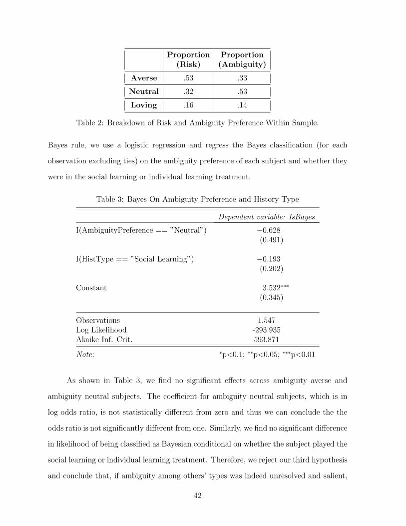
Proportion Proportion(Risk) (Ambiguity)

Averse .53 .33

Neutral .32 .53

Loving .16 .14

Table 2: Breakdown of Risk and Ambiguity Preference Within Sample.

Bayes rule, we use a logistic regression and regress the Bayes classification (for each

observation excluding ties) on the ambiguity preference of each subject and whether they

were in the social learning or individual learning treatment.

Table 3: Bayes On Ambiguity Preference and History Type

Dependent variable: IsBayes

I(AmbiguityPreference == ”Neutral”) −0.628(0.491)

I(HistType == ”Social Learning”) −0.193(0.202)

Constant 3.532∗∗∗

(0.345)

Observations 1,547Log Likelihood -293.935Akaike Inf. Crit. 593.871

Note: ∗p<0.1; ∗∗p<0.05; ∗∗∗p<0.01

As shown in Table 3, we find no significant effects across ambiguity averse and

ambiguity neutral subjects. The coefficient for ambiguity neutral subjects, which is in

log odds ratio, is not statistically different from zero and thus we can conclude the the

odds ratio is not significantly different from one. Similarly, we find no significant difference

in likelihood of being classified as Bayesian conditional on whether the subject played the

social learning or individual learning treatment. Therefore, we reject our third hypothesis

and conclude that, if ambiguity among others’ types was indeed unresolved and salient,

42

then our data cannot be explained by the multiple priors model.

6 Conclusion

In this paper, we introduce two sources of ambiguity in a social learning game and test

whether the multiple priors model in its maximin specification (Gilboa and Schmeidler

1989) is consistent with the data. The model allowed us to make two predictions. First,

as long as it is common knowledge that the precision of the private signal is strictly

greater than 50%, then beliefs, particularly the ”worst prior”, about exact precision do

not affect the players’ strategies. Second, beliefs of others’ rationality does affect the

players’ strategies in the social learning game but not in individual learning game.

We test whether ambiguity over the precision of the private signals has an effect on

behavior and we find that it does not. Although this does not allow us to test the model

directly, any observed differences would suggest that the data is inconsistent with said

model of choice. In addition, we test whether ambiguity over other’s types, which may

characterize a social learning game where only others’ actions are visible, introduced in a

learning game where subjects are either allowed to observe the decisions of past agents or

their private information, has an impact on behavior. The model predicts that ambiguity

should make subjects more likely to deviate from Bayes Rule in favor of their own signal

since the worst prior is that others are irrational (and thus their choices are random). In

this regard, our evidence contradicts the prediction of the multiple priors model. We note,

however, that order and learning effects may have been at play and further research is

needed to distinguish between these. Lastly, we test whether ambiguity-averse subjects,

who are presumably the types of subjects who should more closely behave according to

the multiple priors model, are more likely to deviate from Bayes rule and find that there

is no significant difference between ambiguity averse and ambiguity-neutral subjects.

Broadly speaking, the results of our experiment are inconsistent with the multiple

43

priors models. Perhaps the more striking result is that ambiguity has no significant effect

in social learning. This finding would be consistent with Camerer and Weber (1992)

who suggest that ambiguity aversion has been found to be domain-specific and context-

dependent. In addition, the notion that ambiguity over the precision of the signals is

non-instrumental is not obvious. Thus, it is rather surprising that subjects exhibit no

difference in line with our prediction. Perhaps a word of caution is necessary in in-

terpreting our results since the performance of our subjects - particularly in the social

learning game - is well-above the level recorded in other experiments in the literature.

This may suggest that the college sample used in the experiment may be particularly

sophisticated relative to previous samples and may also reflect why a larger proportion

of subjects were ambiguity neutral relative to those were ambiguity averse. Future ex-

periments should focus on replicating our results with a larger and more diverse sample

given that our findings cast doubt on the effects on ambiguity in an important area of

economic decision-making.

44

Appendix A: Additional Proofs

The proof of Theorem 1 under three additional tie-breaking rules can be found below.

Proof of Theorem 1 under Hci . To establish that γi > (1−γi), it is sufficient to show

Pr(si, Hci |R) > Pr(si, H

ci |B). First, notice that player 1 does not observe a history and,

in the symmetric case, never requires a tie-breaking rule. Therefore, he always chooses

according to his signal since γ1 = p > .5 when s1 = r and γ1 = q < .5 when s1 = b.

Without loss of generality, suppose that s1 = r and thus c1 = R.

Since all subsequent players observe the history of choices, Hci = c1, ..., ci−1, and

not the history of draws, agent i forms beliefs over the probability of observing a given

history conditional on a state. We approach the belief-formation problem of agent i > 1

under three additional tie-breaking rules: the non-confident rule (copies the action of the

previous player), the mixed-confidence rule (subjects act ”non-confident” with probability

δ or ”confident” with probability 1 − δ), and the mixed-color rule (subjects choose Red

with probability δ or Blue with probability 1− δ).

Non-Confident Rule: Assume all subjects are endowed with a non-confident rule

such that if γj = .5 then subject j chooses cj = cj−1. Player 2, knowing that player 1

chooses according to his signal, concludes Pr(Hc2 = R|R) = p and Pr(Hc

2 = R|B) =

q. Therefore, if player 2 receives s2 = r, his choice reduces to γ2 = p2 and 1 − γ2 = pq.

Otherwise, if he receives s2 = b, his posteriors are γ2 = pq = 1− γ2 = pq. In either case,

as long as p > .5, the agent chooses c2 = R. However, note that when the draw of player

2 disagreed with the inferred draw of player 1, the tie-breaking rule was invoked to reach

that conclusion.

Now consider the choice of player 3. He knows player 1 chooses according to his

signal and that player 2’s guess will never differ from player 1’s signal independent of

player 2’s private draw. Therefore, player 3 concludes concludes Pr(Hc3 = R,R|R) =

p(p + q) = p and Pr(Hc3 = R,R|B) = q(q + p) = q. It is now obvious that player

45

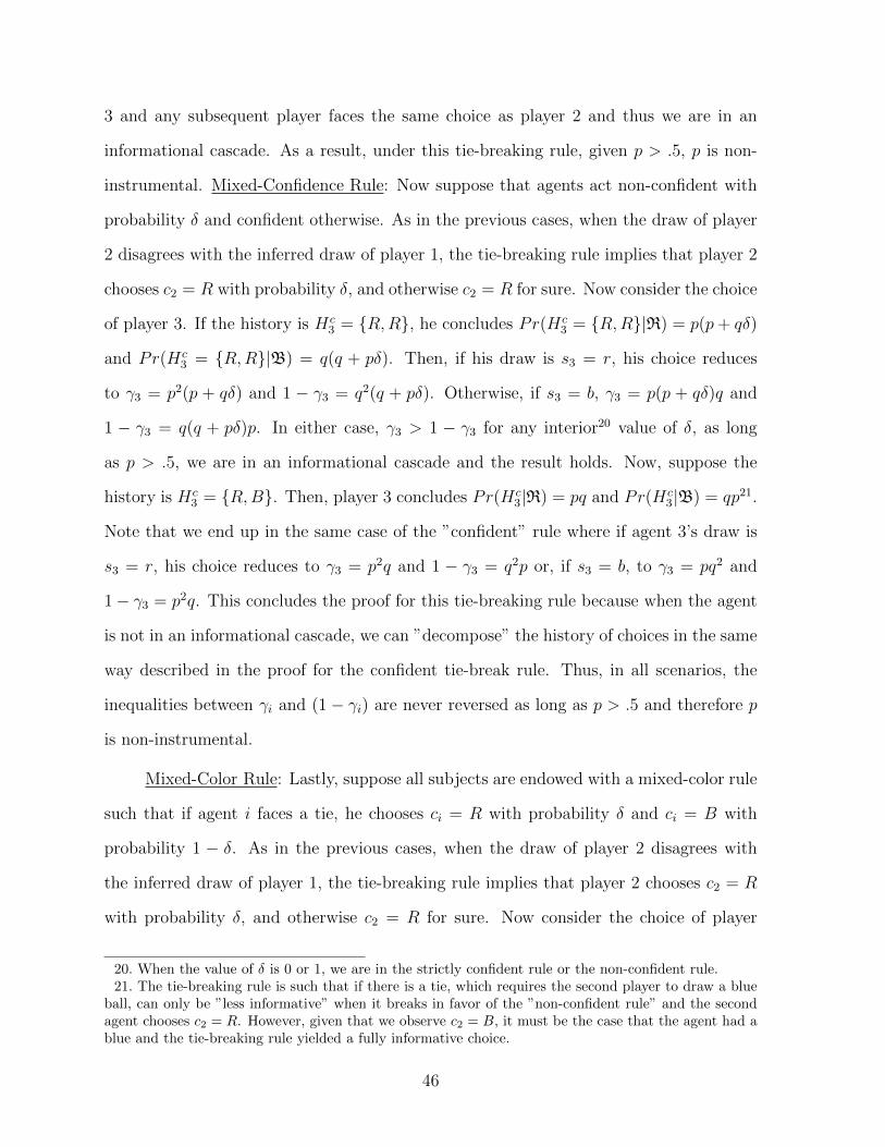
3 and any subsequent player faces the same choice as player 2 and thus we are in an

informational cascade. As a result, under this tie-breaking rule, given p > .5, p is non-

instrumental. Mixed-Confidence Rule: Now suppose that agents act non-confident with

probability δ and confident otherwise. As in the previous cases, when the draw of player

2 disagrees with the inferred draw of player 1, the tie-breaking rule implies that player 2

chooses c2 = R with probability δ, and otherwise c2 = R for sure. Now consider the choice

of player 3. If the history is Hc3 = R,R, he concludes Pr(Hc

3 = R,R|R) = p(p+ qδ)

and Pr(Hc3 = R,R|B) = q(q + pδ). Then, if his draw is s3 = r, his choice reduces

to γ3 = p2(p + qδ) and 1 − γ3 = q2(q + pδ). Otherwise, if s3 = b, γ3 = p(p + qδ)q and

1 − γ3 = q(q + pδ)p. In either case, γ3 > 1 − γ3 for any interior20 value of δ, as long

as p > .5, we are in an informational cascade and the result holds. Now, suppose the

history is Hc3 = R,B. Then, player 3 concludes Pr(Hc

3|R) = pq and Pr(Hc3|B) = qp21.

Note that we end up in the same case of the ”confident” rule where if agent 3’s draw is

s3 = r, his choice reduces to γ3 = p2q and 1 − γ3 = q2p or, if s3 = b, to γ3 = pq2 and

1− γ3 = p2q. This concludes the proof for this tie-breaking rule because when the agent

is not in an informational cascade, we can ”decompose” the history of choices in the same

way described in the proof for the confident tie-break rule. Thus, in all scenarios, the

inequalities between γi and (1− γi) are never reversed as long as p > .5 and therefore p

is non-instrumental.

Mixed-Color Rule: Lastly, suppose all subjects are endowed with a mixed-color rule

such that if agent i faces a tie, he chooses ci = R with probability δ and ci = B with

probability 1 − δ. As in the previous cases, when the draw of player 2 disagrees with

the inferred draw of player 1, the tie-breaking rule implies that player 2 chooses c2 = R

with probability δ, and otherwise c2 = R for sure. Now consider the choice of player

20. When the value of δ is 0 or 1, we are in the strictly confident rule or the non-confident rule.21. The tie-breaking rule is such that if there is a tie, which requires the second player to draw a blue

ball, can only be ”less informative” when it breaks in favor of the ”non-confident rule” and the secondagent chooses c2 = R. However, given that we observe c2 = B, it must be the case that the agent had ablue and the tie-breaking rule yielded a fully informative choice.

46

3. If the history is Hc3 = R,R, he concludes Pr(Hc

3 = R,R|R) = p(p + qδ) and

Pr(Hc3 = R,R|B) = q(q + pδ). Then, if his draw is s3 = r, his choice reduces to

γ3 = p2(p + qδ) and 1 − γ3 = q2(q + pδ). Otherwise, if s3 = b, γ3 = p(p + qδ)q and

1− γ3 = q(q + pδ)p. However, if he observes Hc3 = R,B, he concludes Pr(Hc

3|R) = pq

and Pr(Hc3|B) = qp.22 Then, if his draw is s3 = r, his choice reduces to γ3 = p2q and

1− γ3 = q2p or, if s3 = b, to γ3 = pq2 and 1− γ3 = p2q. In either case, as long as we fix

δ, the inequality over his beliefs (and thus his choice) is unchanged for any p > .5.

An important remark is that when δ ∈ 0, 1, observing ”R” or ”B” in the history

(depending on the value of δ) after a possible tie may be completely uninformative. For

example, when the history shows R,R and δ = 1, the probability of observing ”B” in

the second spot is zero because when there is not tie the second player chooses ”R” and

otherwise he chooses ”R” anyway. A similar conclusion can be extended when δ = 0. To

conclude the proof, suppose that δ ∈ (0, 1) and consider the choice of player 4. First,

notice that for δ ∈ (0, 1), observing a history R,R is sufficient to start a cascade for

player 3 and thus any future agent will also ignore their private information. Therefore,

the only two possible histories of interest are Hc4 = R,B,R and Hc

4 = R,B,B. Close

inspection of the histories makes it evident that the probability of observing these is the

same as if we were observing actual draws, e.g. Pr(Hc4 = R,B,R|R) = qp2. Thus, as

in the case of the ”confident” rule, we can decompose the history and determine whether

these cancel out or not. If we are in an informational cascade then we are done and

otherwise the non-instrumentality of p holds because player 4 faces the same as player 2,

as in the proof used in the main text.

22. Notice that δ is not mentioned anywhere. The logic is as follows, if player 2 had received a draws2 = r given that he observed a history R, his best response is to choose c2 = R. The same is not trueif he had a private draw of s2 = b in which case he would have randomized over which color to choose.

47

Appendix B: Additional Analysis & Plots

Informational Cascades

Since it is not related to our main hypotheses, we not do include the frequency of cas-

cades in the main text. In total, subjects played 240 rounds of the social learning tasks

(ambiguity and risk). In 219 rounds, a cascade formed (about 91.25% of all rounds) and,

within this subset, cascades broke 16.89% of the time for a total of 37 times. We also note

that the probability of a cascade breaking is not significantly different in the ambiguity

trials as compared to the risk trials.

Figure 8: Percent of Bayesian Responses in ILA by Treatment Order & Order in Sequence

Differences ILA and SLR by Order of Treatment

Figures 8 and 9 show the percent of subjects classified as Bayesian in the ILA and SLR

treatments according to the order of the treatments and the order of the subjects in the

sequence.

Notice that any differences in the graphs are minor since, as we mentioned in the

main text, most subjects perform very well in these tasks. Nevertheless, it appears that

48

Figure 9: Percent of Bayesian Responses in SLR by Treatment Order & Order in Sequence

group ”ILR-SLR-ILA-SLA” performs marginally better in most cases. This is due to a

single subject who did very poorly in the game and since all other subjects do extremely

well, this difference is what Figures 8 and 9 are capturing. A logistic regression that

uses robust errors clustered by subject to control for the repeated measures highlights

this point and allows us to conclude that the order of the treatments has no effect on

performance in the SLR and ILA trials beyond that which is attributable to heterogeneity

in the population.

49

Session Code: ILR-ILA-SLR-SLA-AA

1 | P a g e

SL & IL - EXPERIMENT INSTRUCTIONS

INTRO & CONSENT

My name is [NAME] and I am the researcher conducting this experiment. The experiment is about to

begin. Please make yourself comfortable, silence your phones, and don’t talk to each other during the

experiment.

In front of you is a consent form, which briefly summarizes the experiment and your rights as a

participant. Please read it. This copy is for you to sign and to return to us. If you would like a copy for

you to keep, please ask for one at the end of the experiment.

[Wait for participant to read and sign the form]

Your participation in this study is voluntary and you may decide to withdraw at any time. If you agree

to participate and have signed the consent form, please pay attention to the screen in front of the room

while I read the instructions aloud. [*] If you have any questions just raise your hand.

EXPERIMENT OVERVIEW

[*] Today’s experiment will last about 90 minutes. [*] Each of you will receive a show-up fee of $5. In

addition, you will have the chance to earn money during the experiment based on your choices, the

choices of others, and luck. Different participants may earn different amounts. You will be paid at the

end of the experiment in private and in cash and you are under no obligation to tell others how much you

earned.

There will be two parts to the experiment. [*] In the first part, you will play 40 rounds of a game. In each

round, you will be randomly matched with four other players and will then be asked to make one

decision. [*] In the second part, you will participate in a betting task consisting of two questions. You

will provide all your answers through the computer interface in front of you.

Your answers to both parts will determine your final payoff for the experiment in addition to the show-

up fee. You can only gain money; you cannot lose any money. Before I proceed to describe the first part

of the experiment, are there any questions?

[Look around for people raising their hands]

Appendix C: Instructions

50

Session Code: ILR-ILA-SLR-SLA-AA

2 | P a g e

PART I – GENERAL INTRO

[*] I will now read the instructions for PART I. In this part, you will play four types of games. Each

game has 10 rounds. This means that you will complete a total of 40 rounds in this task.

[*] In each round, you will be randomly matched with four other people in the room and ordered in a

random sequence – meaning one person will answer first, another person will answer second, and so on,

until the last answer is provided by the fifth person. You will not know who the other people in your

group are. All groups will face the same task but what happens in other groups has no relevance for

yours.

[*] At the beginning of each round, one of two “jars” will be selected for use during that round. [*] A jar

can be a BLUE jar or a RED jar. Each jar contains 100 balls that may be either red or blue in color. [*]

To determine the composition of the jar chosen in each round, 50 tickets, numbered 51 through 100, will

be placed in a virtual bag and [*] the computer will draw a ticket at random. [*] If the BLUE jar is

chosen, the computer fills the BLUE jar with as many blue balls as indicated by number on the ticket

and fills the rest with red balls. For example, if the BLUE jar is chosen and the number drawn is 75, as

you see on the screen, then the computer fills the jar with 75 blue balls and 25 red balls. [*] Similarly, if

the RED jar is chosen, it fills the RED jar with as many red balls as indicated by number on the ticket

and fills the rest with blue balls. For example, if the RED jar is chosen and the number drawn is 75, as

you see on the screen, then the computer fills the jar with 75 red balls and 25 blue balls.

[*] Notice that the majority of balls is red in the RED jar, and it is blue in the BLUE jar. [*]

Therefore, no matter what jar is chosen, there are always at least 51 balls that match the color of

the jar.

[*] As mentioned before, at the beginning of each round, the computer selects either the RED jar or the

BLUE jar – by flipping a coin. In other words, each jar has the same probability of being chosen. You

will NOT be told in advance which jar has been selected. Instead, you will be asked to guess the identity

of the jar being used for that round.

[*] For this part, your earnings will be denominated in points and will be paid out per the conversion rate

of $1 for every 100 points. This is in addition to your show up fee and your earnings in Part II. You will

earn 50 points for a correct decision and zero points for an incorrect decision. On the screen, a 30-second

timer will help you manage your time while making a choice. [*] Here is what that will look like.

Appendix C: Instructions

51

Session Code: ILR-ILA-SLR-SLA-AA

3 | P a g e

To ensure that we finish the experiment on time, if you take more than a minute to answer, you may be

skipped and you will receive zero points for the round.

[*] Before being asked to make a guess, each of you will be shown on your computer screen a randomly

selected ball from the chosen jar. [*] Once a ball is drawn, it is replaced with a ball of the same color so

that the contents of the jar will be the same whenever another draw is made. [*] Here is an example of

what you will see on your screen. For this subject, who happens to be Player 2, his/her draw is blue.

PART I – INDIVIDUAL LEARNING WITH RISK

[*] In the first game, which corresponds to the first 10 rounds, your screen will indicate the breakdown

of the balls in the jar chosen for the round. [*] For example, if the breakdown of the balls is 88 to 12, as

shown on the screen, it means that if the BLUE jar was chosen for that round, it contains 88 blue balls

and 12 red balls. Otherwise, if the RED jar was chosen, it has 88 red balls and 12 blue balls. Remember

that no matter what jar is chosen, there are always AT LEAST 51 balls that match the color of the jar.

[*] In addition, you will be able to see the private draws of those who went before you (unless you are

the first one to make a choice) and your private draw can be seen by those who go after you. On the

screen, for example, because you are player 2, you can see the draw of player 1. After everyone has made

their guesses, [*] the identity of the chosen jar will be revealed to you on the computer screen. The round

will conclude and the experiment then proceeds to the following round. In the new round, you will again

be matched with other four people and since the match is random, in general, the composition of each

group will change. Again, the computer will choose randomly either the BLUE or RED jar, with equal

probability, and determine the number of red and blue balls in the jar, as previously described.

[*] Are there any questions? [Look around for people raising their hands]

[*] You will now play one practice round. Your will not be compensated for your choice in the practice

round. The purpose of this round is to familiarize you with the computer interface and the rules of the

experiment. Please begin the practice round. [Wait until participants complete the practice rounds]

Does anyone have any questions? [Look around for people raising their hands]

We will now move to the first 10 rounds of Part I of the experiment. Remember that in this part of the

experiment you have the chance to earn bonus money. Please begin.

Appendix C: Instructions

52

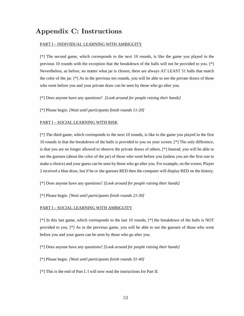
Session Code: ILR-ILA-SLR-SLA-AA

4 | P a g e

PART I – INDIVIDUAL LEARNING WITH AMBIGUITY

[*] The second game, which corresponds to the next 10 rounds, is like the game you played in the

previous 10 rounds with the exception that the breakdown of the balls will not be provided to you. [*]

Nevertheless, as before, no matter what jar is chosen, there are always AT LEAST 51 balls that match

the color of the jar. [*] As in the previous ten rounds, you will be able to see the private draws of those

who went before you and your private draw can be seen by those who go after you.

[*] Does anyone have any questions? [Look around for people raising their hands]

[*] Please begin. [Wait until participants finish rounds 11-20]

PART I – SOCIAL LEARNING WITH RISK

[*] The third game, which corresponds to the next 10 rounds, is like to the game you played in the first

10 rounds in that the breakdown of the balls is provided to you on your screen. [*] The only difference,

is that you are no longer allowed to observe the private draws of others. [*] Instead, you will be able to

see the guesses (about the color of the jar) of those who went before you (unless you are the first one to

make a choice) and your guess can be seen by those who go after you. For example, on the screen, Player

2 received a blue draw, but if he or she guesses RED then the computer will display RED on the history.

[*] Does anyone have any questions? [Look around for people raising their hands]

[*] Please begin. [Wait until participants finish rounds 21-30]

PART I – SOCIAL LEARNING WITH AMBIGUITY

[*] In this last game, which corresponds to the last 10 rounds, [*] the breakdown of the balls is NOT

provided to you. [*] As in the previous game, you will be able to see the guesses of those who went

before you and your guess can be seen by those who go after you.

[*] Does anyone have any questions? [Look around for people raising their hands]

[*] Please begin. [Wait until participants finish rounds 31-40]

[*] This is the end of Part I. I will now read the instructions for Part II.

Appendix C: Instructions

53

Session Code: ILR-ILA-SLR-SLA-AA

5 | P a g e

PART II - AMBIGUITY MEASURE

[*] In this part of the experiment you will be asked to make choices based on the two bags you see at the

front of the room. [*] Bag A and Bag B, each contain 40 poker chips that are either red or blue in color.

I will now describe how each of you will procced to bet on each bag. At the end of the experiment, a

chip will be drawn from each bag and your earning for this part will depend on the color of the chips

drawn and your responses.

First, consider Bag A. [*] In Bag A there are 20 red chips and 20 blue chips. First, you will be asked to

bet on the color of the chip that will be drawn – either a red chip or a blue chip – from each bag. [*] On

the screen, you can see what this will look like. For each gamble, if the chip extracted is of the color you

have bet on, then you win the bet and receive a prize of $2. Otherwise, you lose the bet and get nothing

for that bet. At the end of the experiment, you may inspect the contents of the bag, if you so wish.

Once you have made your bet, you will be presented with a list of choices. [*] This list will ask you to

choose between the gamble and different amounts of money. On the screen, you can see what this will

look like. At the end of Part II, one question from this list will be chosen at random by the computer to

be paid out as follows. If you chose the gamble, then you 'play that gamble', and the amount of money

you win depends on the color of the chip that is extracted. If you chose to take the money, then you

receive that amount of money regardless of the color of the chip drawn.

For example, imagine that you are betting on Bag A which has 20 red and 20 blue chips. Imagine that

(again, for example) you bet that a red chip will be drawn. You are then asked if you would prefer to

keep this gamble, or exchange it for various amounts of money. Suppose that the computer chooses to

pay out the question asking whether you prefer the gamble or $1. If you chose the money, you will get

$1, regardless of the color of the chip drawn. However, if you chose to keep the gamble, then you will

receive $2 if a red chip is drawn and $0 otherwise.

[*] Are there any questions? [Look around for people raising their hands]

[*] For Bag B, you will also be asked to make bet and to choose between the gamble and various amounts

of money. In other words, the betting procedure will be identical, but the contents of Bag B may be

different than those of Bag A. In Bag B the number of red and blue chips is unknown. It could be ANY

number between 0 red chips (with 40 blue chips) and 40 red chips (with 0 blue chips).

Appendix C: Instructions

54

Session Code: ILR-ILA-SLR-SLA-AA

6 | P a g e

What you know about the content of each bag will appear on your computer screen when you make

decisions about that bag. [*] Are there any questions? [Look around for people raising their hands]

[*] Please begin the experiment. [Wait until participants complete PART 2]

CONCLUSION:

[*] This is the end of the experiment. I will now ask one of you to come up to the front to draw a chip

from each bag to determine the outcome of the bet and use it to calculate the final payment. Then we

will pay each of you in private in the next room according to your computer number. Please do not use

the computer; be patient, and remain seated until we call you to be paid.

Appendix C: Instructions

55

Experimental InstructionsBy: Luis Sanchez (01.22.17)

ILR-ILA-SLR-SLA-AA

Put All Electronic Devices On Silent

No Cellphones Allowed During the Experiment

Summary of Experiment

The experiment will last approximately 90 minutes.

In addition to your $5 show-up fee, you can earn money

during the experiment.

For Part I, you will be matched with 4 other players and

in each round you will be asked to make one decision.

For Part II, you will complete an individual betting task.

Instructions for Part I

In each round, you are randomly matched with four

other people in the room.

At the beginning of each round, the computer selects

one of two jars: either a RED jar or a BLUE jar.

RED BLUE ...

Appendix C: Accompanying Visuals

56

BLUEHere is an example…

RED

And another example…

RED BLUE

Here is the example when the ticket is 75…

Instructions for Part I

In each round, you are randomly matched with four other people in the room.

At the beginning of each round, the computer selects one of two jars: either a RED jar or a BLUE jar.

Each jar has 100 balls out of which the majority of balls

Each jar is equally likely to be chosen. Your job is to guess the color of the jar being used in that round.

If you guess correctly, you get 50 points. Otherwise, you get zero. You will be paid $1 for every 100 points.

Appendix C: Accompanying Visuals

57

OR OOR

GAME 1

Rounds #1-10

Appendix C: Accompanying Visuals

58

Are there any questions?

PPART I: Reminders for Rounds 1-110At the beginning of each round, the computer selects one of two jars:

either a RED jar or a BLUE jar. Each jar is equally likely to be chosen.

Each jar has 100 balls out of which the majority of balls (>50) match

the color of the urn.

You WILL BE provided the breakdown of balls in the jar being used.

You will be able to see the private DRAWS of those who went before

you and your private DRAW can be seen by those who go after you.

For each round, if you guess correctly, you get 50 points. Otherwise,

you get zero. You will be paid $1 for every 100 points.

GAME 2

Rounds #11-20

Appendix C: Accompanying Visuals

59

Are there any questions?

PPART I: Reminders for Rounds 11-220At the beginning of each round, the computer selects one of two jars:

either a RED jar or a BLUE jar. Each jar is equally likely to be chosen.

Each jar has 100 balls out of which the majority of balls (>50) match

the color of the urn.

You WON’T be provided the breakdown of balls in the jar being used.

You will be able to see the private DRAWS of those who went before

you and your private DRAW can be seen by those who go after you.

For each round, if you guess correctly, you get 50 points. Otherwise,

you get zero. You will be paid $1 for every 100 points.

GAME 3

Rounds #21-30

Red

Appendix C: Accompanying Visuals

60

Are there any questions?

PPART I: Reminders for Rounds 21-330At the beginning of each round, the computer selects one of two jars:

either a RED jar or a BLUE jar. Each jar is equally likely to be chosen.

Each jar has 100 balls out of which the majority of balls (>50) match

the color of the urn.

You will be provided the breakdown of balls in the jar being used.

You will be able to see the private draws of those who went before

you and your private draw can be seen by those who go after you.

For each round, if you guess correctly, you get 50 points. Otherwise,

you get zero. You will be paid $1 for every 100 points.

GAME 4

Rounds #31-40

Are there any questions?

Appendix C: Accompanying Visuals

61

PPART I: Reminders for Rounds 31-440At the beginning of each round, the computer selects one of two jars:

either a RED jar or a BLUE jar. Each jar is equally likely to be chosen.

Each jar has 100 balls out of which the majority of balls (>50) match

the color of the urn.

You will be provided the breakdown of balls in the jar being used.

You will be able to see the private draws of those who went before

you and your private draw can be seen by those who go after you.

For each round, if you guess correctly, you get 50 points. Otherwise,

you get zero. You will be paid $1 for every 100 points.

This is the end of Part I.

We will now proceed with Part II of the experiment.

= 40+ = 40+

BBag A

= 20= 20

= 40+

or

Appendix C: Accompanying Visuals

62

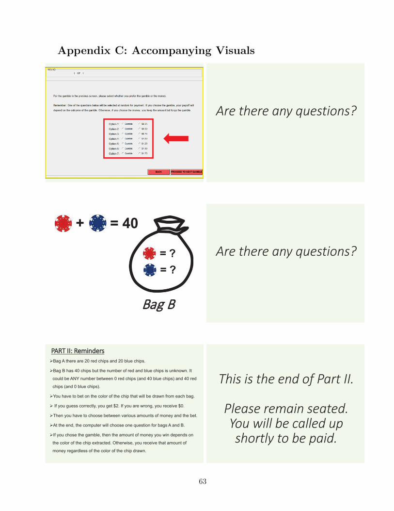
Are there any questions?

BBag B

= ?= ?

= 40+

Are there any questions?

PPART II: RemindersBag A there are 20 red chips and 20 blue chips.

Bag B has 40 chips but the number of red and blue chips is unknown. It

could be ANY number between 0 red chips (and 40 blue chips) and 40 red

chips (and 0 blue chips).

You have to bet on the color of the chip that will be drawn from each bag.

If you guess correctly, you get $2. If you are wrong, you receive $0.

Then you have to choose between various amounts of money and the bet.

At the end, the computer will choose one question for bags A and B.

If you chose the gamble, then the amount of money you win depends on

the color of the chip extracted. Otherwise, you receive that amount of

money regardless of the color of the chip drawn.

This is the end of Part II.

Please remain seated.You will be called up shortly to be paid.

Appendix C: Accompanying Visuals

63

References

Anderson, Lisa R., and Charles A. Holt. 1997. “Information Cascades in the Laboratory.”

The American Economic Review 87 (5): 847–862. http://www.jstor.org/stable/

2951328.

Banerjee, Abhijit V. 1992. “A Simple Model of Herd Behavior.” The Quarterly Journal

of Economics 107 (3): 797–817. http://www.jstor.org/stable/2118364.

Becker, Selwyn W., and Fred O. Brownson. 1964. “What Price Ambiguity? or the Role of

Ambiguity in Decision-Making.” Journal of Political Economy 72 (1): 62–73. doi:10.

1086/258854.

Bikhchandani, Sushil, David Hirshleifer, and Ivo Welch. 1992. “A Theory of Fads, Fash-

ion, Custom, and Cultural Change as Informational Cascades.” Journal of Political

Economy 100 (5): 992–1026. http://www.jstor.org/stable/2138632.

Camerer, Colin, and Martin Weber. 1992. “Recent developments in modeling preferences:

Uncertainty and ambiguity.” Journal of Risk and Uncertainty 5 (4): 325–370. doi:10.

1007/BF00122575.

Celen, Bogachan, and Shachar Kariv. 2004. “Distinguishing Informational Cascades from

Herd Behavior in the Laboratory.” American Economic Review 94 (3): 484–498.

doi:10.1257/0002828041464461.

Chow, Clare Chua, and Rakesh K. Sarin. 2001. “Comparative Ignorance and the Ellsberg

Paradox.” Journal of Risk and Uncertainty 22 (2): 129–139. doi:10.1023/A:101115

7509006.

Curley, Shawn P., and J.Frank Yates. 1989. “An empirical evaluation of descriptive mod-

els of ambiguity reactions in choice situations.” Journal of Mathematical Psychology

33, no. 4 (December): 397–427. doi:10.1016/0022-2496(89)90019-9.

Dean, Mark., and Pietro Ortoleva. 2016. “Is it All Connected? A Testing Ground for

Unified Theories of Behavioral Economics Phenomena.” http://www.columbia.

edu/~po2205/papers/DeanOrtoleva_Relationship.pdf.

Dijk, Eric van, and Marcel Zeelenberg. 2003. “The discounting of ambiguous information

in economic decision making.” Journal of Behavioral Decision Making 16 (5): 341–

352. doi:10.1002/bdm.450.

64

Ellsberg, Daniel. 1961. “Risk, Ambiguity, and the Savage Axioms.” Quarterly Journal of

Economics 75 (4): 643–669. http://www.jstor.org/stable/1884324.

Epstein, Larry G., and Martin Schneider. 2007. “Learning Under Ambiguity.” Review of

Economic Studies 74 (4): 1275–1303. doi:10.1111/j.1467-937X.2007.00464.x.

Ergin, Haluk, and Faruk Gul. 2009. “A theory of subjective compound lotteries.” Journal

of Economic Theory 144 (3): 899–929. doi:10.1016/j.jet.2008.08.003.

Fischbacher, Urs. 2007. “z-Tree: Zurich toolbox for ready-made economic experiments.”

Experimental Economics 10 (2): 171–178. doi:10.1007/s10683-006-9159-4.

Fox, Craig R., and Amos Tversky. 1995. “Ambiguity Aversion and Comparative Igno-

rance.” The Quarterly Journal of Economics 110 (3): 585–603.

Fox, Craig R, and Martin Weber. 2002. “Ambiguity aversion, comparative ignorance, and

decision context.” Organizational Behavior and Human Decision Processes 88 (1):

476–498. doi:10.1006/obhd.2001.2990.

Gilboa, Itzhak, and David Schmeidler. 1989. “Maxmin expected utility with non-unique

prior.” Journal of Mathematical Economics 18 (2): 141–153. doi:10.1016/0304-

4068(89)90018-9.

Goeree, Jacob K., Thomas R. Palfrey, Brian W. Rogers, and Richard D. McKelvey. 2007.

“Self-Correcting Information Cascades.” Review of Economic Studies 74 (3): 733–

762. doi:10.1111/j.1467-937X.2007.00438.x.

Goeree, Jacob K., and Leeat Yariv. 2015. “Conformity in the lab.” Journal of the Eco-

nomic Science Association 1 (1): 15–28. doi:10.1007/s40881-015-0001-7.

Granovetter, Mark S. 1978. “Threshold Models of Collective Behavior.” American Journal

of Sociology 83 (6): 1420–1443. doi:10.1086/226707.

Heath, Chip, and Amos Tversky. 1991. “Preference and belief: Ambiguity and competence

in choice under uncertainty.” Journal of Risk and Uncertainty 4 (1): 5–28. doi:10.

1007/BF00057884.

Ivanov, Asen. 2011. “Attitudes to ambiguity in one-shot normal-form games: An exper-

imental study.” Games and Economic Behavior 71 (2): 366–394. doi:10.1016/j.

geb.2010.05.009.

65

Kelsey, David, and Sara LeRoux. 2015. “An experimental study on the effect of ambiguity

in a coordination game.” Theory and Decision 79 (4): 667–688. doi:10.1007/s11238-

015-9483-2.

Knight, Frank H. 1921. Risk, Uncertainty, and Profit. Houghton Mifflin Company.

Koessler, Frederic, and Anthony Ziegelmeyer. 2000. “Tie-breaking Rules and Informa-

tional Cascades: A Note.” https://ideas.repec.org/p/ulp/sbbeta/2000-

09.html.

Machina, Mark J., and Marciano Siniscalchi. 2014. “Ambiguity and ambiguity aversion.”

In Handbook of the Economics of Risk and Uncertainty, 1:729–807. North Holland.

isbn: 9780444536853.

Miller, John H., and Scott E. Page. 2004. “The standing ovation problem.” Complexity

9 (5): 8–16. doi:10.1002/cplx.20033.

Moreno, OM, and Yaroslav Rosokha. 2015. “Learning Under Compound Risk vs. Learning

Under Ambiguity-An Experiment.” http://www.krannert.purdue.edu/centers/

vseel/papers/LearnCvU.pdf.

Schmeidler, David. 1989. “Subjective Probability and Expected Utility without Additiv-

ity.” Econometrica 57 (3). doi:10.2307/1911053.

Segal, Uzi. 1987. “The Ellsberg Paradox and Risk Aversion: An Anticipated Utility Ap-

proach.” International Economic Review 28 (1): 175. doi:10.2307/2526866.

Trautmann, Stefan T., and Richard J. Zeckhauser. 2013. “Shunning uncertainty: The

neglect of learning opportunities.” Games and Economic Behavior 79 (1): 44–55.

doi:10.1016/j.geb.2013.01.001.

Yates, J Frank, and Lisa G Zukowski. 1976. “Characterization of ambiguity in decision

making.” Behavioral Science 21 (1): 19–25. doi:10.1002/bs.3830210104.

Zappia, Carlo. 2015. “Daniel Ellsberg on the Ellsberg Paradox.” PhD diss., University of

Siena.

66