amber 6.2 verification summary - quintessa limited verification... · qe-amber-3, verification...

AMBER 6.2 Verification Summary

QE-AMBER-3

Version 6.2

August 2017

QE-AMBER-3, Verification Summary, Version 6.2

i

Summary

AMBER is a compartment modelling software tool developed by Quintessa Ltd.

This is the Verification Summary for the AMBER 6.2 software. AMBER 6.2 is a flexible

software tool that allows the user to build their own dynamic compartment models to

represent the migration and fate of contaminants in a system.

© Quintessa Limited. All rights reserved. Quintessa Limited owns the rights to AMBER.

See Help | About AMBER for license information.

Quintessa Limited

The Hub

14 Station Road

Henley-on-Thames

Oxfordshire RG9 1AY

United Kingdom

Phone: +44 (0)1925 885956

email: [email protected]

https://www.quintessa.org/AMBER

mailto:[email protected]


ii

Contents

1 INTRODUCTION ......................................................................................................................................................... 1

2 PUBLISHED APPLICATIONS .................................................................................................................................. 3

3 SIMPLE TEST CASES .................................................................................................................................................. 5

3.1 SN2 .................................................................................................................................................................... 5 3.2 SN5 .................................................................................................................................................................... 6 3.3 SN7 .................................................................................................................................................................... 7

4 LEVEL 1B ........................................................................................................................................................................ 12

4.1 DETERMINISTIC ............................................................................................................................................... 12 4.2 STOCHASTIC .................................................................................................................................................... 14

5 SOLUBILITY LIMITED CASE ................................................................................................................................. 15

5.1 TOXICITY ......................................................................................................................................................... 15 5.2 EFFECTIVE LEACH RATE ................................................................................................................................ 15 5.3 RESULT OF COMPARISON .............................................................................................................................. 15

6 LANGMUIR AVAILABILITY TEST ...................................................................................................................... 18

6.1 SIMPLE LIMITING CASE .................................................................................................................................. 18 6.2 SHARED LANGMUIR CASE............................................................................................................................. 19

7 CHECK OF PROBABILITY DISTRIBUTIONS .................................................................................................. 21

7.1 UNIFORM......................................................................................................................................................... 21 7.2 LOG UNIFORM ................................................................................................................................................ 22 7.3 GAUSSIAN ....................................................................................................................................................... 23 7.4 LOG GAUSSIAN ............................................................................................................................................... 24 7.5 TRUNCATED GAUSSIAN................................................................................................................................. 25 7.6 TRIANGULAR .................................................................................................................................................. 25 7.7 LOG TRIANGULAR .......................................................................................................................................... 27 7.8 BETA ................................................................................................................................................................ 27 7.9 LOG BETA ........................................................................................................................................................ 28 7.10 GENERAL CDF ............................................................................................................................................... 28 7.11 LOG GENERAL CDF ....................................................................................................................................... 29

8 CORRELATION CHECKS ........................................................................................................................................ 30

8.1 INDEPENDENT SAMPLING ............................................................................................................................. 30 8.2 SPECIFYING CORRELATIONS.......................................................................................................................... 30

9 PRESSURE TESTS ....................................................................................................................................................... 32

9.1 TRANSFER RATES............................................................................................................................................ 32 9.2 COMPARTMENTS ............................................................................................................................................ 32 9.3 CONTAMINANTS AND DECAYS .................................................................................................................... 32 9.4 LARGE NUMBERS ........................................................................................................................................... 33 9.5 SOLVER TOLERANCE ...................................................................................................................................... 33

10 AMBER 6.2 SPATIAL PARAMETERS TESTS .................................................................................................... 35

10.1 ISAM VAULT TEST CASE .............................................................................................................................. 35 10.2 NON-CUBOID GEOMETRY ............................................................................................................................. 38


iii

11 AMBER 6.2 TARGETED TESTS .............................................................................................................................. 40

11.1 BASIC PARAMETER FUNCTIONALITY ........................................................................................................... 40 11.2 GUI PROPERTIES AND FUNCTIONALITY ...................................................................................................... 40 11.3 CALCULATION AND OUTPUT TESTS ............................................................................................................. 41 11.4 OTHER TESTS .................................................................................................................................................. 41

12 CONCLUSIONS .......................................................................................................................................................... 42

REFERENCES ...................................................................................................................................................................... 42


1

1 Introduction

The AMBER compartment modelling code is a general-purpose tool. It allows the

development of compartment models, and calculation of their solutions, for a wide range of

situations. Details of AMBER and its use are provided in Quintessa (2017a and b).

The verification of such a computer tool is essentially a matter of demonstrating that the code

does what it claims. That is, the models are solved correctly in accordance with what has

been specified. The verification of the models themselves, as opposed to the computer code,

is the responsibility of the model developer who uses AMBER.

However, in the process of verifying specific models, users are implicitly verifying the correct

functioning of the underlying tool. In this way, every application of AMBER builds

confidence in the tool itself. This is particularly true when intercomparisons with other codes

are performed and when checks against analytic solutions are made.

Some published applications of AMBER involving such intercomparisons are discussed in

Section 2.

In addition to the ongoing use of the tool, it is useful to have a set of test cases specifically

developed to check the correct functioning of the code. Various tests have been developed.

This document brings together a standard set of these tests and reports on their application

to AMBER 6.2. These tests have been carried out for both the Windows and Linux versions

of AMBER 6.2. This report is accompanied by electronic versions of the AMBER case files,

which are referred to in the documentation of each test and are installed with the software.

The AMBER 6.0 release in December 2015 included a completely new user interface. An

extensive set of tests were developed to help ensure the correct operation of the user interface.

The AMBER 6.2 release has also been subject to the same suite of user interface tests under

both Windows and Linux, though the numerous tests are not described here. The tests

described in this report focus on checking that the correct solution is calculated by AMBER.

The tests described here are as follows.

Some simple cases with known solutions that have been used throughout AMBER’s

development are described in Section 3.

The Nuclear Energy Agency (NEA) PSAG Level 1B exercise, which checks the

deterministic and probabilistic functioning of AMBER against the documented results

from a number of participant members of the PSAG group, are described in Section 4.

A comparison with a solubility-limited source term model, developed by

AEA Technology for Nirex is described in Section 5.

A comparison with a spreadsheet calculation for a case involving a Langmuir

Availability scheme is given in Section 6.

A case using all of the available probability distributions to check that sensible values are

generated is described in Section 7.


2

Section 8 describes the results of cases used to test that sampling is properly random and

that correlations are appropriately generated when specified.

These cases all perform well and give confidence in the correct functioning of the code.

In addition, Section 9 describes the results of ‘pressure testing’ of the code and solvers to

determine some of the practical limits for aspects including transfer rates, number handling,

contaminants and transfers. Section 10 summarises some tests that check the correct

calculation of spatial properties in AMBER 6.2. Section 11 summarises additional tests for

AMBER 6.2.

Brief conclusions are presented in Section 12, whilst references are provided at the end of the

report.


3

2 Published Applications

AMBER has been applied in many projects. The AMBER User Guide (Quintessa, 2017b)

includes a list of publications that describe assessments in which AMBER has been applied.

The following is a short selection of those that include comparisons with other codes.

As part of SKI's review of SKB's calculations for the SFR 1 repository for low and intermediate

level waste, AMBER was used to undertake an exploration of some of the important issues

(Maul and Robinson, 2002). As well as demonstrating the applicability of AMBER in an

overall performance assessment, the calculations include direct comparisons with SKB

calculations. Given the slightly different modelling assumptions that were made, the results

agree well.

AMBER has since been used by SSM as part of their review of SKB’s calculations for the KBS-

3 repository for spent fuel, considering both near-field processes and radionuclide transport

(Penfold, 2014) and landscape modelling and dose assessment calculations (Walke, 2014;

Walke and Limer, 2014; Walke et al., 2015). It was also used by STUK in their review of

Posiva’s TURVA-12 assessment for the spent fuel geological disposal facility at Olkiluoto,

with a focus on the radionuclide transport modelling (Towler et al., 2014). These reviews

consisted a test of both the conceptual modelling approaches adopted by the waste

management organisations, SKB and Posiva, but also a test of their calculations against

independent calculations undertaken using AMBER.

In addition, SKI and SSI have undertaken an intercomparison between AMBER and Ecolego

to give confidence in their application to total-system performance assessment (PA) studies

for deep repositories and to further review SKB’s SR 97 calculations (Maul et al., 2003 and

2004). The studies compared the results for near-field, geosphere and biosphere

implementations, considering both deterministic and probabilistic calculations. The studies

demonstrated good agreement between the two codes.

SKB have used AMBER as the benchmark against which to test their Tensit simulation tool

(Jones et al., 2004). The study demonstrates excellent agreement between the two codes.

AMBER was successfully used in the Vault Test Case of the IAEA’s ISAM programme to

model the migration and fate of liquid and solid releases from a near-surface radioactive

waste repository (IAEA, 2003a). The results obtained from AMBER were in agreement with

those obtained using other internationally recognised codes.

AMBER was used in support of the IAEA’s BIOMASS programme (IAEA, 2003b). The

results for Example Reference Biospheres (ERBs) 2A and 2B were obtained following their

implementation in AMBER. Very close agreement was achieved when the AMBER results

for ERB 2A were compared with the results achieved following its implementation in a

different software package.

The performance of AMBER was evaluated against the Pacific Northwest Laboratory’s

MEPAS code and Andra’s AQUABIOS code in assessing the environmental impact of non-


4

radioactive contaminants (Côme et al., 2004, ANDRA, 2003). The project demonstrated close

agreement between AMBER and the other codes.

Models developed using AMBER have been compared against other models in BIOMOVS II.

QuantiSci (now Enviros Consulting Limited) developed an AMBER model for the C-14

release to a lake scenario (BIOMOVS, 1996a), whilst Ciemat (Spain) developed models for the

Complementary Studies (BIOMOVS, 1996b) and lysimeter (BIOMOVS, 1996c) exercises.

In work for the FSA (formerly MAFF), AMBER cases were developed to reproduce earlier

results produced by the MAFF H3 and C14 STAR codes (Watkins et al., 1998). The results

were reproduced precisely.

AMBER models, in conjunction with models from IPSN and ANDRA (France) have been

used in an IAEA study to derive activity limits for the near-surface disposal of radioactive

waste (IAEA, 2003c).

In an application to subsurface transport, AMBER models have also been used by an MSc

student to represent the migration of contaminants in an aquifer and the results successfully

compared against analytical solutions (Scott, 1998).


5

3 Simple Test Cases

3.1 SN2

This case is a simple system with three compartments and two contaminants (see

Figure 1). The transfer rates are piecewise constant. Results (amount of each contaminant in

each compartment against time) were calculated with the SPADE code (a general differential

equation solver) (Williams and Woods, 1994) and compared to those obtained using AMBER.

Figure 1. Structure of SN2

A B

C

Compartments Contaminants

Nuc1

Nuc2

Nuc1 decays at a rate of 1E-4 per year and Nuc2 at a rate of 1E-2 per year.

The source to A is for Nuc1 only. It is zero except for two time intervals: from 0 to 10 years

it is 1 mol/y, and from 30 to 50 years it is 2 mol/y.

This test case is implemented in SN2.cse. The initial transfer rates are given in the

Table 1. After 40 years they all fall by a factor of 100.

Table 1. Initial Transfer Rates for SN2

Transfer Initial Transfer Rate (per year)

From To Nuc1 Nuc2

A B 0.01 0.001

B C 0.001 0.1

C A 0.1 0.1

Results are calculated at 10, 20, 30, 40, 50 and 100 years.

The 10 and 100 year results are quoted as representative in Table 2. Differences from the

SPADE results are shown by highlighting the digits that differ. Results (amounts in moles)


6

with both AMBER’s Laplace and time-stepping solver are compared to 6 significant figures.

The agreement is very good throughout.

Table 2. Comparison of SN2 Results with SPADE (moles)

Comp-

artment

Conta-

minant

Tim

e

SPADE AMBER (Windows) AMBER (Linux)

Laplace

Solver

Time-step

Solver

Laplace

Solver

Time-step

Solver

A Nuc1 10 9.51191 9.51191 9.51191 9.51191 9.51191

A Nuc2 10 0.00466821 0.00466821 0.00466821 0.00466821 0.00466821

B Nuc1 10 0.481807 0.481807 0.481807 0.481807 0.481807

B Nuc2 10 0.000137848 0.000137849 0.000137849 0.000137849 0.000137849

C Nuc1 10 0.00128303 0.00128305 0.00128305 0.00128305 0.00128305

C Nuc2 10 2.97304E-5 2.97307E-5 2.97310E-5 2.97307E-5 2.97310E-5

A Nuc1 100 45.5501 45.5501 45.5501 45.5501 45.5501

A Nuc2 100 0.220230 0.220230 0.220229 0.220230 0.220229

B Nuc1 100 4.09113 4.09113 4.09114 4.09113 4.09114

B Nuc2 100 0.0188336 0.0188336 0.0188335 0.0188336 0.0188335

C Nuc1 100 0.0249555 0.0249555 0.0249547 0.0249555 0.0249547

C Nuc2 100 0.00142203 0.00142203 0.00142206 0.00142203 0.00142206

3.2 SN5

SN5 tests a simple case with non-depleting transfers and local decay rates; the structure is

illustrated in Figure 2.

Nuc1 decays at a rate of 0.01 per year in compartment A only. The transfers are both non-

depleting and have a rate of 1 per year. Thus, B calculates the integral of A; and C calculates

the integral of B. Initially, there is 1 mole of Nuc1 in A.

The solution is simply:

2

1

1

t

t

t

etC

eB

eA

where is the decay rate.

This test case is implemented in SN5.cse. The Laplace solver and time-step solver have both

been used to calculate the amount of Nuc1 (moles) in each compartment as a function of time.


7

The results are compared with an analytical solution in Table 3. The agreement is very good

throughout.


A B

C

Compartments Contaminants

Nuc1

Table 3. Results of SN5 (moles)

Time Compartme

nt

Analytic AMBER (Windows) AMBER (Linux)

Laplace

Solver

Time-step

Solver

Laplace

Solver

Time-step

Solver

0.01 A 0.999900 0.999900 0.999900 0.999900 0.999900

0.01 B 0.00999950 0.00999950 0.00999949 0.00999950 0.00999949

0.01 C 4.99983E-5 4.99983E-5 5.05133E-5 4.99983E-5 5.05133E-5

10 A 0.904837 0.904837 0.904837 0.904837 0.904837

10 B 9.51626 9.51626 9.51626 9.51626 9.51626

10 C 48.3742 48.3742 48.3742 48.3742 48.3742

100 A 0.367879 0.367879 0.367872 0.367879 0.367872

100 B 63.2121 63.2121 63.2128 63.2121 63.2128

100 C 3678.79 3678.79 3678.72 3678.79 3678.72

1000 A 4.53999E-5 4.53999E-5 4.61771E-5 4.53999E-5 4.61771E-5

1000 B 99.9955 99.9955 99.9954 99.9955 99.9954

1000 C 90000.5 90000.5 90000.5 90000.5 90000.5

3.3 SN7

SN7 is a case with a loop of compartments with identical transfer rates and a non-decaying

contaminant. A general analytic solution can be found for any number of compartments.

Here, 12 have been used (see Figure 3).


8


A1 A2

A12

A3

A9 A8 A7

A11

A10

A4

A5

A6

All the transfer rates are 0.1 per year and the initial amounts are: 1 mol in A1, A2, A4, A6, A7

and A10; zero elsewhere.

The analytic result for a general system with N compartments in a loop and a transfer rate of

is derived as follows.

The equation for the amount in compartment n is:

1 nn

n AAdt

dA

where A0 and AN are equivalent. We look for eigen-solutions with:

t

nn eEtA )(

from the governing equation it is clear that:

1

nn EE

and the loop symmetry gives:

1

N

.

The eigen-values are therefore given by:

)1( /.2)( Nkik e

with corresponding eigen-solutions:


9

Nnkik

n eE /..2)( .

This then leads to the solution:

tN

k

k

n

k

n

k

eEtA)(

1

)()()(

,

where:

N

n

k

nn

k EAN 1

)()( )0(1

.

From this, results at 20, 40, 60, 80 and 100 have been calculated. These are presented in

Table 4.

Table 4. Analytical Results for SN7

Compartment Amounts (moles)

t=20 t=40 t=60 t=80 t=100

A1 0.331448 0.393231 0.493590 0.545518 0.541057

A2 0.500565 0.382391 0.450256 0.521544 0.542698

A3 0.578488 0.421262 0.422288 0.489768 0.532723

A4 0.598713 0.483640 0.421521 0.460279 0.513205

A5 0.544824 0.530970 0.445906 0.443184 0.489534

A6 0.533186 0.548898 0.481307 0.443560 0.468849

A7 0.634764 0.561520 0.514184 0.459365 0.457322

A8 0.647070 0.584441 0.540759 0.484075 0.457839

A9 0.491510 0.589493 0.561193 0.510966 0.469434

A10 0.419087 0.556907 0.570820 0.534847 0.488415

A11 0.400650 0.503189 0.562832 0.551199 0.509930

A12 0.319694 0.444059 0.535343 0.555695 0.528994

The test case is implemented in AMBER in SN7.cse and the results, using the time-step solver,

are shown in Table 5. The digits that disagree are highlighted.


10

Table 5. AMBER Results for SN7 [Identical for Windows and Linux OS]


t=20 t=40 t=60 t=80 t=100

A1 0.331439 0.393228 0.493591 0.545508 0.541053

A2 0.500576 0.382384 0.450256 0.521533 0.542690

A3 0.578493 0.421278 0.422296 0.489764 0.532711

A4 0.598697 0.483641 0.421539 0.460290 0.513196

A5 0.544834 0.530961 0.445919 0.443209 0.489540

A6 0.533181 0.548888 0.481297 0.443584 0.468872

A7 0.634769 0.561518 0.514158 0.459366 0.457353

A8 0.647075 0.584458 0.540749 0.484052 0.457857

A9 0.491499 0.589501 0.561213 0.510944 0.469429

A10 0.419083 0.556886 0.570833 0.534847 0.488397

A11 0.400666 0.503184 0.562819 0.551208 0.509914

A12 0.319687 0.444074 0.535331 0.555695 0.528988

The agreement is generally to 3-4 significant figures, with no deterioration for larger times.

As an experiment, an extra disconnected transfer was added with a faster transfer rate (10).

This causes AMBER to take shorter time-steps, at least initially. This change is implemented

in SN7(Extra).cse and the calculated results are shown in Table 6.


11

Table 6. AMBER Results for SN7 with a Faster Transfer Rate Added [Identical for

Windows and Linux OS]


t=20 t=40 t=60 t=80 t=100

A1 0.331440 0.393228 0.493590 0.545509 0.541053

A2 0.500576 0.382384 0.450256 0.521533 0.542689

A3 0.578492 0.421277 0.422296 0.489764 0.532710

A4 0.598697 0.483641 0.421539 0.460289 0.513196

A5 0.544835 0.530961 0.445919 0.443208 0.489540

A6 0.533180 0.548888 0.481297 0.443583 0.468873

A7 0.634770 0.561518 0.514159 0.459366 0.457353

A8 0.647075 0.584457 0.540749 0.484053 0.457857

A9 0.491499 0.589500 0.561212 0.510945 0.469429

A10 0.419083 0.556887 0.570833 0.534847 0.488397

A11 0.400666 0.503184 0.562820 0.551207 0.509914

A12 0.319687 0.444073 0.535331 0.555695 0.528988

These results are very similar to those presented in Table 5, with only small differences at the

sixth significant figure.


12

4 Level 1B

PSAG Level 1B has a biosphere model with multiple transfers, compartments and

contaminants. Transfer rates are specified as formulae. The exercise was organised by the

NEA PSAG (Probabilistic Safety Assessment Group) (NEA, 1993).

Deterministic and probabilistic results are given.

4.1 Deterministic

Initially, a precise match could not be obtained. Further investigation revealed three small

errors in the printed Level1B report that explain this. The errors are: in equation 16, tan

should be sin ; and in equations 37 and 38 where the denominators should match the food

type.

Having corrected these, the rates quoted in Table B5 of NEA (1993) are matched.

Table D1 of NEA (1993) gives the Bq inventories at a number of times. The participants

generally agree. This test case is implemented in Level1B.cse and the deterministic results are

generated by calculating Level1B.cse with the ‘Best Estimates’ sampling option selected in the

Calculate dialogue. The base units for the model are moles (see Section 4.3.1 of the Reference

Guide), the compartment amounts in Bq are given in the parameter M_comp. The AMBER

results using the Laplace solver are compared against the AEAT results using MASCOT in

Table 7, as this is a semi-analytic solution and should be the most accurate and can be directly

compared.

Table 7. Comparison of AMBER and Mascot Amounts for Level1B [Identical for

Windows and Linux OS]

Time AMBER: Amount (Bq) MASCOT: Amount (Bq)

1 1000 100000 1 1000 100000

Nuclide Compartment: Water

C14 4.67E+3 2.71E+3 2.20E-3 4.66E+3 2.70E+3 2.19E-3

U235 3.42E+0 9.69E+0 7.56E+0 3.41E+0 9.67E+0 7.55E+0

Pa231 7.25E-5 2.32E-1 6.58E+0 7.24E-5 2.32E-1 6.57E+0

Ac227 1.14E-6 2.16E-1 6.19E+0 1.14E-6 2.16E-1 6.18E+0

Nuclide Compartment: Sediment

C14 1.20E+3 3.87E+3 3.14E-3 1.20E+3 3.86E+3 3.13E-3

U235 8.70E-1 1.08E+1 8.46E+0 8.68E-1 1.08E+1 8.45E+0

Pa231 1.63E-5 2.62E-1 7.48E+0 1.62E-5 2.62E-1 7.46E+0

Ac227 2.30E-7 2.08E-1 6.00E+0 2.30E-7 2.08E-1 5.99E+0


13

Time AMBER: Amount (Bq) MASCOT: Amount (Bq)

1 1000 100000 1 1000 100000

Nuclide Compartment: TopSoil

C14 1.80E+6 2.76E+9 5.11E+3 1.81E+6 2.76E+9 5.11E+3

U235 4.64E+2 4.88E+7 5.66E+7 4.64E+2 4.88E+7 5.66E+7

Pa231 9.78E-3 1.24E+6 4.93E+7 9.78E-3 1.24E+6 4.93E+7

Ac227 1.54E-4 1.14E+6 4.62E+7 1.54E-4 1.14E+6 4.63E+7

Nuclide Compartment: DeepSoil

C14 2.21E+8 1.21E+11 2.24E+5 2.21E+8 1.21E+11 2.24E+5

U235 1.63E+5 1.06E+8 1.13E+8 1.63E+5 1.06E+8 1.13E+8

Pa231 3.45E+0 2.00E+6 6.81E+7 3.45E+0 1.80E+6 6.82E+7

Ac227 5.42E-2 2.00E+6 7.12E+7 5.42E-2 2.00E+6 7.12E+7

The only significantly different result is for Pa-231 in Deep Soil at 1000 years. Other

participants give the result as 2.00E+6, in agreement with AMBER, so it is supposed that the

quoted result quoted for MASCOT is probably erroneous.

Given the good match seen here, the dose results should match well. A full set of results is

given in Section D2 of NEA (1993). This is confirmed by a few spot checks. In Table 8 the

U-235 decay pathway (D_Path[U_235]) results are compared in detail.

Table 8. Comparison of AMBER and Mascot Dose Rates for Level1B

Time AMBER (Windows):

Dose (Sv/y)

AMBER (Linux):

Dose (Sv/y)

MASCOT:

Dose (Sv/y)

1 1000 100000 1 1000 100000 1 1000 100000

Water 5.1E-12 1.4E-11 1.1E-11 5.1E-12 1.4E-11 1.1E-11 5.1E-12 1.4E-11 1.1E-11

Fish 1.1E-12 3.1E-12 2.4E-12 1.1E-12 3.1E-12 2.4E-12 1.1E-12 3.1E-12 2.4E-12

Grain 1.5E-13 1.8E-9 2.1E-9 1.5E-13 1.8E-9 2.1E-9 1.5E-13 1.8E-9 2.1E-9

Meat 7.0E-12 1.6E-8 1.8E-8 7.0E-12 1.6E-8 1.8E-8 7.0E-12 1.6E-8 1.8E-8

Milk 4.5E-14 9.9E-11 1.2E-10 4.5E-14 9.9E-11 1.2E-10 4.5E-14 9.9E-11 1.1E-10

Dust 1.9E-14 2.0E-9 2.3E-9 1.9E-14 2.0E-9 2.3E-9 1.9E-14 2.0E-9 2.3E-9

Externa

l

3.9E-14 4.1E-9 4.8E-9 3.9E-14 4.1E-9 4.8E-9 4.0E-14 4.2E-9 4.8E-9


14

4.2 Stochastic

For stochastic results, a precise match is not expected. Most participants used 1000 samples,

so the AMBER results are also generated using 1000 samples with the ‘Full’ Sampling option

selected in the Calculate dialogue and a seed of 987654321 (see Section 7.2.3 of the Reference

Guide).

Table D3 of NEA (1993) gives the results for C14 total dose and U235 chain total dose.

The mean results obtained with AMBER are compared against the range of means obtained

by participants using Monte Carlo analysis.

Table 9. Mean Stochastic Results for Level1B [Identical for Windows and Linux OS]

Time AMBER: Total dose (Sv/y) Participants: Total dose (Sv/y)

C14 U235 Chain C14 U235 Chain

1 1.53E-7 2.30E-11 1.3E-7 to 1.5E-7 2.1E-11 to 2.3E-11

3 6.92E-7 2.95E-11 6.1E-7 to 7.0E-7 2.8E-11 to 3.0E-11

10 2.79E-6 8.94E-11 2.5E-6 to 2.8E-6 8.1E-11 to 9.0E-11

30 8.70E-6 4.36E-10 7.8E-6 to 8.7E-6 4.0E-10 to 4.4E-10

100 2.79E-5 2.67E-9 2.5E-5 to 2.8E-5 2.6E-9 to 2.7E-9

300 7.15E-5 1.57E-8 6.5E-5 to 7.1E-5 1.5E-8 to 1.6E-8

1000 1.40E-4 1.29E-7 1.3E-4 to 1.4E-4 1.3E-7 to 1.4E-7

3000 1.15E-4 8.92E-7 1.1E-4 to 1.1E-4 8.8E-7 to 9.5E-7

10000 2.56E-5 5.96E-6 2.5E-5 to 2.7E-5 6.0E-6 to 6.5E-6

30000 1.12E-6 2.03E-5 1.1E-6 to 1.2E-6 2.1E-5 to 2.3E-5

100000 9.23E-11 2.05E-5 7.9E-11 to 1.0E-10 2.2E-5 to 2.4E-5

300000 * 3.12E-6 * 3.3E-6 to 4.2E-6

1000000 * 2.03E-7 * 1.7E-7 to 3.0E-7

*Result very small

The AMBER results for both C-14 and the U-235 chain agree well with the range reported by

the PSACOIN Level 1B participants.


15

5 Solubility Limited Case

In this section, a comparison is made with a published report on a solubility limited source

model developed for Nirex and other UK organisations (Robinson et al, 1988), which is

referred to here by its reference number, R11854.

R11854 reports on a solubility limited source term model.

The results are calculated using the time-step solver for 55 nuclides, including stable species.

R11854 omits to give the U-233 inventory, which has been set to give the same peak toxicity

for Th-229.

5.1 Toxicity

R11854 gives maximum near-field Toxicity and Time of Occurrence for each nuclide where

the maximum is more than 0.1.

This test case is implemented in R11854.cse and the results can be directly compared with

those from R11854 (see Table 10).

5.2 Effective Leach Rate

R11854 gives initial and maximum effective leach rate (to 106 years) for each element. These

can be directly compared (see Table 11).

5.3 Result of Comparison

The comparison with R11854 gives generally good agreement. The discrepancies could be

caused by data errors in the original report or by numerical issues. None are serious enough

to cause any concern.


16

Table 10. Comparison of AMBER Maximum Toxicity with R11854

Nuclide AMBER (Windows) AMBER (Linux) R11854

Maximum

Toxicity

Time of

Occurrence

Maximum

Toxicity

Time of

Occurrence

Maximum

Toxicity

Time of

Occurrence

C14 2.72E+1 300 2.72E+1 300 2.73E+1 300

Se79 1.05E+1 300 1.05E+1 300 1.05E+1 300

Sr90 9.70E+3 300 9.70E+3 300 9.70E+3 300

Nb93m 3.47E+3 300 3.47E+3 300 3.48E+3 300

Nb94 2.22E+4 300 2.22E+4 300 2.22E+4 300

Tc99 3.17E-1 300 3.17E-1 300 3.17E-1 300

Sn126 3.33E+1 300 3.33E+1 300 3.33E+1 300

I129 5.35E+1 300 5.35E+1 300 5.36E+1 300

Cs135 4.41E+0 300 4.41E+0 300 4.42E+0 300

Cs137 8.66E+3 300 8.66E+3 300 8.67E+3 300

Pb210 7.14E+4 300 7.14E+4 300 7.16E+4 300

Ra226 2.52E+3 300 2.52E+3 300 2.53E+3 300

Ac227 2.87E+1 300000 2.87E+1 300000 2.90E+1 3E+5

Th229 7.31E+1 34756 7.31E+1 34756 7.31e+1 4E+4

Th230 2.21E+0 406040 2.21E+0 406040 2.20E+0 5E+5

Pa231 2.02E+1 300000 2.02E+1 300000 2.04E+1 3E+5

Np237 1.68E+1 3000 1.68E+1 3000 1.68E+1 3E+3

Pu238 6.94E-1 300 6.94E-1 300 6.73E-1 300

Pu239 1.33E+1 40944.8 1.33E+1 40944.8 1.33E+1 5E+4

Pu240 9.28E+0 300 9.28E+0 300 8.96E+0 300

Pu242 7.32E-1 269554* 7.32E-1 269554* 6.57E-1 3E+5

Am241 1.28E+3 300 1.28E+3 300 1.28E+3 300

Am242

m

9.64E-1 300 9.64E-1 300 7.97E-1 300

Am243 4.11E+0 1311.13* 4.11E+0 1311.13* 3.84E+0 1E+3

Note: * These values would round to the value reported for R11854 and are therefore considered

consistent.


17

Table 11. Comparison of AMBER Leach Rates with R11854 (y-1)

Element AMBER (Windows) AMBER (Linux) R11854

Initial

Leach Rate

Maximum

Leach Rate

Initial

Leach Rate

Maximum

Leach Rate

Initial

Leach Rate

Maximum

Leach Rate

H 8.0E-3 8.0E-3 8.0E-3 8.0E-3 Not given Not given

C 8.1E-4 7.7E-3 8.1E-4 7.7E-3 8.1E-4 7.7E-3

Ni 8.2E-9 8.3E-9 8.2E-9 8.3E-9 8.2E-9 8.3E-9

Se 7.7E-3 7.7E-3 7.7E-3 7.7E-3 7.7E-3 7.7E-3

Sr 1.6E-3 1.6E-3 1.6E-3 1.6E-3 1.6E-3 1.6E-3

Zr 1.3E-7 1.5E-7 1.3E-7 1.5E-7 1.3E-7 1.5E-7

Nb 7.7E-3 7.7E-3 7.7E-3 7.7E-3 7.7E-3 7.7E-3

Tc 1.5E-5 2.0E-4 1.5E-5 2.0E-4 1.5E-5 2.0E-4

Sn 7.7E-3 7.7E-3 7.7E-3 7.7E-3 7.7E-3 7.7E-3

I 7.7E-3 7.7E-3 7.7E-3 7.7E-3 7.7E-3 7.7E-3

Cs 1.6E-3 1.6E-3 1.6E-3 1.6E-3 1.6E-3 1.6E-3

Sm 2.7E-9 2.7E-9 2.7E-9 2.7E-9 2.7E-9 2.7E-9

Pb 7.7E-3 7.7E-3 7.7E-3 7.7E-3 7.7E-3 7.7E-3

Ra 1.6E-3 1.6E-3 1.6E-3 1.6E-3 1.6E-3 1.6E-3

Ac 2.0E-4 2.0E-4 2.0E-4 2.0E-4 2.0E-4 2.0E-4

Th 2.0E-6 2.0E-6 2.0E-6 2.0E-6 2.0E-6 2.0E-6

Pa 2.0E-4 2.0E-4 2.0E-4 2.0E-4 2.0E-4 2.0E-4

U 2.3E-13 2.3E-13 2.3E-13 2.3E-13 2.3E-13 2.3E-13

Np 2.0E-6 2.0E-6 2.0E-6 2.0E-6 2.0E-6 2.0E-6

Pu 7.5E-9 2.0E-6 7.5E-9 2.0E-6 7.3E-9 2.0E-6

Am 4.5E-7 2.0E-6 4.5E-7 2.0E-6 4.5E-7 2.0E-6

Cm 2.0E-6 2.0E-6 2.0E-6 2.0E-6 2.0E-6 2.0E-6


18

6 Langmuir Availability Test

In order to test the correct functioning of the Langmuir Availability scheme, two cases have

been run.

The first uses a limiting case to give an analytic result. The second compares the results of a

shared scheme with a separately coded solution (using a larger number of simple timesteps).

6.1 Simple Limiting Case

For a single compartment and contaminant, with a source, Langmuir-controlled loss rate and

decay constant, the equation for the amount is:

A

AAsA

dt

dA.

In the limit as 0 this becomes simply:

sAdt

dA)( .

In the case where s , the solution is simply:

teAA )(

0

,

where 0A is the initial amount.

Here 10 A , 001.0 , 01.0 , 5.0 and 2010 . The last of these is chosen to be

as close to zero as possible (AMBER does not allow a zero value). A good match is expected

for all times when A .

The test case is implemented in SimpleLimitingCase.cse and the results using the time-step

solver can be directly compared with the analytical solution (see Table 12). As can be seen,

the match is very good throughout.


19

Table 12. AMBER and Analytical Results for Simple Langmuir Solutions (moles)

Time AMBER

(Windows)

AMBER

(Linux)

Analytic Ratio

0 1.000E+0 1.000E+0 1.000E+0 1.000

1 9.891E-1 9.891E-1 9.891E-1 1.000

2 9.782E-1 9.782E-1 9.782E-1 1.000

5 9.465E-1 9.465E-1 9.465E-1 1.000

10 8.958E-1 8.958E-1 8.958E-1 1.000

20 8.025E-1 8.025E-1 8.025E-1 1.000

50 5.770E-1 5.770E-1 5.769E-1 1.000

100 3.329E-1 3.329E-1 3.329E-1 1.000

200 1.108E-1 1.108E-1 1.108E-1 1.000

500 4.086E-3 4.086E-3 4.087E-3 1.000

1000 1.669E-5 1.669E-5 1.670E-5 0.999

1200 1.849E-6 1.849E-6 1.850E-6 0.999

1500 6.808E-8 6.808E-8 6.830E-8 0.997

2000 2.761E-10 2.761E-10 2.790E-10 0.990

6.2 Shared Langmuir Case

In this test, there are two contaminants with a shared Langmuir scheme. The two have

different decay rates and there are different sources. The first contaminant decays to the

second. The equations solved are:

BA

BAAsA

dt

dAAAA

BA

BABsBA

dt

dBBBBA

In the absence of analytic results, a small spreadsheet has been created that solves these

equations using small explicit steps.

The data used is as follows. Here 10 A , 20 B , 001.0A , 003.0B , 01.0A ,

005.0B , 002.0As , 001.0Bs , 5.0 and 1 .

The results tend to a steady state where the source balances the decay and loss rates.

The spreadsheet results are calculated with a step of 0.1. Each step consists of an explicit

forward step from which an approximate average value over the step is obtained. This is

then used for the full step.


20

This test case is implemented in SharedLangmuirCase.cse and the results using the time-step

solver can be directly compared with the analytical solution (see Table 13). The agreement

obtained is excellent, confirming the correct behaviour of the Langmuir calculation.

Table 13. AMBER and Analytical Results for Shared Langmuir Schemes (moles)

Time AMBER

(Windows)

AMBER (Linux) Analytic Ratio

(Analytic/Linux)

A B A B A B A B

0 1.00000 2.00000 1.00000 2.00000 1.00000 2.00000 1.00000 1.00000

1 0.99229 1.98730 0.99229 1.98730 0.99229 1.98730 1.00000 1.00000

2 0.98466 1.97468 0.98466 1.97468 0.98466 1.97468 1.00000 1.00000

5 0.96226 1.93739 0.96226 1.93739 0.96226 1.93739 1.00000 1.00000

10 0.92646 1.87702 0.92646 1.87702 0.92645 1.87702 1.00001 1.00000

20 0.86027 1.76267 0.86027 1.76267 0.86027 1.76267 1.00000 1.00000

50 0.69876 1.46548 0.69876 1.46548 0.69876 1.46548 1.00000 1.00000

100 0.52012 1.09340 0.52012 1.09340 0.52013 1.09341 0.99998 0.99999

200 0.34989 0.65116 0.34989 0.65116 0.34990 0.65117 0.99997 0.99998

500 0.26256 0.26215 0.26256 0.26215 0.26256 0.26215 1.00000 1.00000

1000 0.26317 0.20302 0.26317 0.20302 0.26316 0.20302 1.00004 1.00000

2000 0.26365 0.20081 0.26365 0.20081 0.26365 0.20081 1.00000 1.00000

5000 0.26365 0.20081 0.26365 0.20081 0.26365 0.20081 1.00000 1.00000

10000 0.26365 0.20081 0.26365 0.20081 0.26365 0.20081 1.00000 1.00000


21

7 Check of Probability Distributions

In order to test the correct functioning of the sampling distributions, a test has been run with

each type of distribution, in both standard and log-based form. This test case has been

implemented and saved as PDFs.cse. A large number of samples (10,000) have been used to

get good statistics, note that the sampled parameters can be checked by checking the ‘Do not

calculate’ box in the Calculate dialogue.

The mean and certain percentiles are evaluated and exported from AMBER using the

statistical report and CDF plot functions.

7.1 Uniform

A uniform distribution in the range 1 to 3 is used. The min and max should be very close to

the limits for 10000 samples (a few times 1E-4 typically). The mean and median should be

very close to 2.0. The 25th and 75th percentiles should be close to 1.5 and 2.5.

The reported values (when using either the Windows and Linux operating systems) are:

Monte Carlo Latin Hypercube

Min 1.0001 1.0002

25% 1.5045 1.4999

50% 2.0113 1.9999

Mean 2.0000 2.0000

75% 2.4921 2.5000

Max 2.9999 3.0000

which all seem sensible.

The number of samples below 2.0 is 4941 with full Monte Carlo sampling. For a binomial

distribution we expect a deviation about the mean (5000) of 10000/5000 , which is 50, so

the observed deviation of 59 is entirely plausible. In addition to the test above, the Latin

Hypercube option was tested with the same uniform distribution but with only 100 samples.

Figure 4 shows the frequency distribution generated by Monte Carlo sampling, whereas

Figure 5 shows the result for Latin Hypercube sampling. The figures confirm the stratified

sampling that is achieved with the Latin Hypercube approach.


22

Figure 4. Uniform Distribution, Monte Carlo Sampling

Figure 5. Uniform Distribution, Latin Hypercube Sampling

7.2 Log Uniform

A log-based uniform in the range 10-6 to 10-2 is used. The min and max should be close to the

limits. The median should be close to 10-4, while the 25th and 75th percentiles are close to 10-5

and 10-3. The mean should be (10-2-10-6)/ln(104), which is 1.0856 10-3.

The reported values (when using either the Windows and Linux operating systems) are:


Min 1.0001E-6 1.0007E-6

25% 1.0491E-5 9.9965E-6

50% 9.7383E-5 9.9949E-5

Mean 1.0794E-3 1.0856E-3

75% 9.8118E-4 9.9908E-4

Max 9.9994E-3 9.9971E-3

which are all sensible.


23

The number of samples below 10-4 is 5047 with full Monte Carlo sampling. As described

above, for a binomial distribution we expect a deviation 50 , so the observed deviation of

47 is entirely plausible.

7.3 Gaussian

A full Gaussian has no upper and lower limits. We choose a mean of 10 and a standard

deviation of 2. The min and max could be as many as 4 standard deviations from the mean

(i.e. 2 and 18).

The mean and median should be close to 10. The 25th and 75th percentiles should be 8.651 and

11.349.

The reported values (when using the Windows operating system) are:


Min 2.9001 1.7104

25% 8.6482 8.6504

50% 10.0212 10.0000

Mean 10.0161 10.0000

75% 11.3774 11.3484

Max 17.7345 17.9078

which are all sensible. The values reported when using the Linux operating system were

almost identical, with the exception of the Min value with the Monte Carloe sampling; in that

instance a value of 2.9001 was reported.

The number of samples below 10 is 4953 with full Monte Carlo sampling. As described above,

for a binomial distribution we expect a deviation 50 , so the observed deviation of 47 is

entirely plausible.

In addition to the test above, the Latin Hypercube option was tested with the same Gaussian

distribution but with only 100 samples. Figure 6 shows the frequency distribution generated

by Monte Carlo sampling, whereas Figure 7 shows the result for Latin Hypercube sampling.

The figures confirm the stratified sampling that is achieved with the Latin Hypercube

approach.


24

Figure 6. Gaussian Distribution, Monte Carlo Sampling

Figure 7. Gaussian Distribution, Latin Hypercube Sampling

7.4 Log Gaussian

For the Log Gaussian we choose a distribution with a log with mean 3 and standard deviation

1. The min should be around 0.1, the max 107. The median should be 103 and the 25th and 75th

percentiles should be 211.6 and 4726. Then mean should be 1.417E+4.

The reported values (when using either the Windows or Linux operating systems) are:


Min 0.13431 0.11091

25% 202.51 211.46

50% 983.36 999.84

Mean 1.2347E+4 1.3805E+4

75% 4835.2 4724.7

Max 1.9748E+6 7.8770E+6



25

The number of samples below 1000 is 5024 with full Monte Carlo sampling. As described

above, for a binomial distribution we expect a deviation 50 , so the observed deviation of

24 is entirely plausible.

7.5 Truncated Gaussian

A truncated Gaussian has upper and lower limits. We choose the same mean and standard

deviation as the Gaussian test (10 and 2), but with a range of 8 to 16 (i.e. 1 standard deviation

below and 3 above).

The statistics for this are hard to calculate. Min and max will be near to 8 and 16. The 25th,,

50th and 75th percentiles are 9.329, 10.397 and 11.603. The mean is 10.566.



Min 8.0000 8.0006

25% 9.3327 9.3290

50% 10.4065 10.3966

Mean 10.5612 10.5656

75% 11.5995 11.6033

Max 15.9799 15.9871


The number of samples below the median (10.397) is 4977 with full Monte Carlo sampling.

As described above, for a binomial distribution we expect a deviation 50 , so the observed

deviation of 23 is entirely plausible.

7.6 Triangular

The triangular distribution has a minimum, a peak, and a maximum. For the test, we choose

11, 14 and 15. This has the 75th percentile at 14, the 25th and median at 12.7321 and 13.4495.

The mean is 13.3333.



Min 11.0429 11.0047

25% 12.7079 12.7319

50% 13.4377 13.4494

Mean 13.3255 13.3333

75% 14.0166 13.9998

Max 14.9861 14.9861



26




In addition to the test above, the Latin Hypercube option was tested with the same triangular

distribution but with only 100 samples. Figure 6 shows the frequency distribution generated

by Monte Carlo sampling, whereas Figure 7 shows the result for Latin Hypercube sampling.

The figures confirm the stratified sampling that is achieved with the Latin Hypercube

approach.

Figure 8. Triangular Distribution, Monte Carlo Sampling

Figure 9. Triangular Distribution, Latin Hypercube Sampling


27

7.7 Log Triangular

The log triangular distribution has a minimum, a peak, and a maximum for the logarithm.

For the test, we choose 1, 2 and 4, giving a range from 10 to 104. The 25th, 50th and 75th

percentiles are 73.46, 185.33 and 596.01. The mean is 611.10.



Min 10.071 10.030

25% 75.499 73.432

50% 188.79 185.33

Mean 621.21 611.12

75% 607.32 596.01

Max 9387.0 9715.8





7.8 Beta

The beta distribution has a minimum, and a maximum with two parameters, A and B

controlling the shape of the distribution. For the test, we choose a range –4 to –2 with A and

B set to 0.5 and 1.5.

The 25th, 50th and 75th percentiles are -3.922, -3.674 and -3.194. The mean is -3.5.



Min -4.0000 -4.0000

25% -3.9214 -3.9219

50% -3.6601 -3.6737

Mean -3.4946 -3.5000

75% -3.1839 -3.1945

Max -2.0073 -2.0051

which are all sensible. The minimum being at -4 is because of the choice of A smaller than 1.

This gives a singularity in the density at the end and thus generates values very close to the

limit.


28

The number of samples below the median (-3.674) is 4905 with full Monte Carlo sampling.



7.9 Log Beta

For the log beta test, we use the same parameters as the beta test, but for the log.

The 25th, 50th and 75th percentiles are 1.197E-4, 2.120E-4 and 6.393E-4. The mean is 7.32E-4.



Min 1.0000E-4 1.0000E-4

25% 1.1931E-4 1.1970E-4

50% 2.0787E-4 2.1200E-4

Mean 7.3186E-4 7.3225E-4

75% 6.3156E-4 6.3918E-4

Max 9.8269E-3 9.8643E-3


The number of samples below the median (2.12E-4) is 5072 with full Monte Carlo sampling.



7.10 General CDF

The General CDF allows a piecewise linear CDF to be specified. This corresponds to a

piecewise constant PDF (histogram). The test uses four equi-probable intervals, 1 to 2, 2 to 4,

4 to 7 and 7 to 8.

The 25th, 50th and 75th percentiles are at the interval boundaries: 2, 4 and 7. The mean is 4.375.



Min 1.0011 1.0004

25% 1.9857 1.9998

50% 4.0480 3.9998

Mean 4.3795 4.3750

75% 7.0029 6.9999

Max 8.0000 7.9999



29

The number of samples below the median (4) is 4955 with full Monte Carlo sampling. As

described above, for a binomial distribution we expect a deviation 50 , so the observed


7.11 Log General CDF

For the Log General CDF we take the intervals (of the log) as –1 to 0, 0 to 1 and 1 to 1.6. We

assign probabilities of 0.3, 0.5 and 0.2 to these.

The 25th, 50th and 75th percentiles are 0.6813, 2.5119 and 7.943. The min and max are 0.1 and

39.811. The mean is 6.3871.



Min 0.1000 0.1000

25% 0.6598 0.6810

50% 2.4719 2.5116

Mean 6.4095 6.3871

75% 7.9123 7.9429

Max 39.7915 39.798






30

8 Correlation Checks

This section describes verification tests that demonstrate:

that parameters are sampled independently; and

that correlations can be specified.

8.1 Independent Sampling

To check that the separate sampled values are not correlated, two Gaussian distributions

were generated, both with zero mean and unit variance and saved as NoCorrelationCheck.cse.

The standard and rank correlation coefficients were generated in batch mode with a 10,000

sample Monte Carlo run:

Standard correlation coefficient: -0.0013473

Rank correlation coefficient: -0.00263604

Similarly, standard and rank correlation coefficients were generated in batch mode with a

10,000 sample Latin Hypercube run:

Standard correlation coefficient: -0.0072046

Rank correlation coefficient: -0.00443935

These results indicate a very low correlation, as expected. The same results were recorded

when using either the Windows or Linux operating systems.

8.2 Specifying Correlations

The ability to specify rank correlation coefficients has been tested by setting up a simple case

with the parameters and correlations defined in Table 14. The specification therefore includes

two separate correlation sets (Ppt, RunOff and Irrig forming one group and Kd and CF_Plant

another), positive and negative correlations and different types of distribution.

Table 14. Definition of Parameters and Correlation Coefficients

Name Distribution Correlation

Ppt Gaussian: mean = 0.98, SD = 0.095, minimum = 0

RunOff Gaussian: mean = 0.31, SD = 0.08, minimum = 0 To Ppt = 0.8

Irrig Triangular: peak = 0.3, minimum = 0, maximum = 0.6 To Ppt = -0.9

To RunOff = -0.85

Kd Lognormal: GM = 0.018, GSD = 10

CF_Plant 0.03, GSD = 10 To Kd = -0.7

The case, CorrelationCheck.cse, was run with 10,000 samples. The resulting matrix of rank

correlation coefficients is shown in Table 15 and proves a good match to those specified in


31

Table 14. The table also provides confidence that no correlations are introduced between the

separate parameter groups, with a maximum rank correlation coefficient of -0.0022, which is

very low.

Table 15. Matrix of Rank Correlation Coefficients [Same for both Windows and Linux

operating systems]

Parameter Ppt Irrig RunOff Kd CF_Plant

Ppt 1 -0.9070 0.8075 -1e-005 -0.0013

Irrig -0.9070 1 -0.8536 -0.0005 0.0014

RunOff 0.8075 -0.8536 1 -0.0022 -0.0005

Kd -1e-005 -0.0005 -0.0022 1 -0.6913

CF_Plant -.0.0013 0.0014 -0.0005 -0.6913 1


32

9 Pressure Tests

A further requirement of the AMBER 6.2 verification is pressure testing, in order to document

the limits of the AMBER software in performing calculations and inform sensible application

of the code. These tests look at the limits of transfer rates, number of compartments, number

of contaminants and decays, user-entered large numbers, and at the issues of memory

leakage and solver tolerance. The results are reported below.

The nature of pressure testing requires that large cases be used for some of the tests, some of

these have been based on extensions of commercial cases and are therefore not available for

distribution with the other verification cases. These cases are noted below.

9.1 Transfer Rates

A simple case, PressureTest_TransferRate.cse, was set up to investigate whether a maximum

limit is encountered for the rate of transfers. The case has two compartments and one

transfer. The transfer is configured as non-depleting, as the large fluxes expected would soon

empty a depleting compartment.

In this configuration, running the calculation with a transfer rates above 1.3E+154 y-1 using

the Laplace solver caused the calculation to be halted and a series of error messages to appear.

Up to and including this value, the calculations ran as expected. Such a rapid transfer is well

beyond the bounds of sensible application.

When using the Time-Step solver, no problems were encountered before reaching the limit

of large numbers (see below).

9.2 Compartments

The maximum number of compartments that AMBER can handle is largely a function of the

computer system used and its available memory. Whilst it is difficult to identify a set limit of

compartments, many models have been run comfortably with large numbers of

compartments. For example, a recent commercial application includes 452 compartments

and is run without any problems on a Microsoft Windows machine with 3GB of RAM. Also,

a case with a single contaminant and a chain of over 1000 compartments operates as expected.

9.3 Contaminants and Decays

A recent commercial case file, developed for screening radionuclides, includes 1070

contaminants and 1160 decays. The case was extended to investigate whether limits are

encountered for the number of contaminants and decays. The contaminants and decays were

duplicated and the case was run until errors were reported. No problems were encountered

up to and including a case where 5350 contaminants and 5800 decays were used. This

provides evidence that AMBER can handle a large number of contaminants and decays, well

beyond the bounds of expected application.


33

9.4 Large Numbers

Using the simple case PressureTest_TransferRate.cse, described above, start amounts and

transfer rates were increased to see how AMBER handles large numbers. Up to and

including values of 1E+308, the values were stored fine (regardless of units). However, above

these values, the editor stored them as ”1.#INF“ (infinity). Even before calculations were run,

the editor was unable to store larger numerical values; the program unsurprisingly prevents

the results from being calculated and displays an error message when trying to use values of

infinity. A similar process occurs in batch mode; when the file is re-saved the value of infinity

replaces any numbers greater than 1E+308. This is because the software saves values to

double-precision, and 1E+308 is the maximum that can be stored in the allocated memory for

this format – it is sufficiently large, however, to be unlikely to cause any problems.

9.5 Solver Tolerance

AMBER cases may involve simultaneous handling of both large and small numbers, differing

by many orders of magnitude, in and between a system of compartments. The AMBER

solvers, as with any numerical solvers, need to include a level of tolerance in relation to such

situations.

A test case, PressureTest_SolverTolerance.cse is set up to examine the practical implications of

the AMBER solver tolerances, comprising of a single contaminant moving between two

compartments with a transfer rate of 1 y-1. There is a source flux of this contaminant into the

first compartment at a rate equal to sin²(t) mol y-1, keeping the amount of contaminant in this

compartment relatively constant, oscillating around ~0.5 mol. In the second compartment

different start amounts are set, increasing from zero up to higher powers of ten. Monitoring

the reported values in the first compartment then demonstrates the tolerance of the solver –

as long as the values are reported as expected then the solver can handle the calculations, but

if the values in the first compartment are not what is expected, then it can be seen that the

solver cannot handle both the smaller fluxes into the first compartment and the large values

held in the second compartment.

The calculations report values as expected up until the second compartment contains 1E+9

moles of contaminant. Above this (i.e., when there were around 10 or more orders of

magnitude between the largest and smallest values in the system), the reported values for the

first compartment deviated significantly, as can be seen by the green line in Figure 10. For

values of 1E+11 mol and above (11 or more orders of magnitude between the largest and

smallest values in the system), the model broke down and gave entirely incorrect results, as

shown by the yellow line in Figure 10.

This test case indicates that the accuracy of AMBER may begin to break down when

evaluating amounts of contaminants that are more than ten orders of magnitude below the

highest amounts in the system. Such solver tolerances are unavoidable and the results for

AMBER are considered acceptable because such very small amounts are unlikely to be of

interest in most applications. However, the results highlight the importance of exploring and


34

questioning the results of any numerical code, including AMBER. Should such small results

be related to observers of interest, then the modelling approach warrants further iteration, for

example, by separating the part of the system where very small amounts are calculated into

a separate AMBER model and importing fluxes from the source term.

It is emphasised that the solver tolerance is not a weakness in AMBER, but a practical issue

that is relevant to any numerical solvers. Indeed, it is noted in Section 2 that AMBER

performs very well in relation to other codes and even provides the benchmark against which

other codes have been tested.

Figure 10. Solver Tolerance Test Results showing Calculated Amount in Compartment 1

with Deferring Initial Amounts in Compartment 2


35

10 AMBER 6.2 Spatial Parameters Tests

A major new feature since the release of AMBER 6.0 is the addition of spatial awareness.

Compartments can be assigned spatial dimensions from which AMBER is able to calculate a

range of properties, including compartment volumes, interface areas and transfer distances.

These spatial parameters are tested by comparison with analytical calculations of the same

properties.

10.1 ISAM Vault Test Case

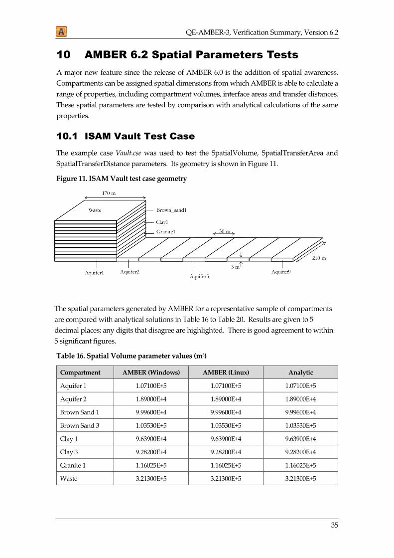
The example case Vault.cse was used to test the SpatialVolume, SpatialTransferArea and

SpatialTransferDistance parameters. Its geometry is shown in Figure 11.

Figure 11. ISAM Vault test case geometry

The spatial parameters generated by AMBER for a representative sample of compartments

are compared with analytical solutions in Table 16 to Table 20. Results are given to 5

decimal places; any digits that disagree are highlighted. There is good agreement to within

5 significant figures.

Table 16. Spatial Volume parameter values (m3)

Compartment AMBER (Windows) AMBER (Linux) Analytic

Aquifer 1 1.07100E+5 1.07100E+5 1.07100E+5

Aquifer 2 1.89000E+4 1.89000E+4 1.89000E+4

Brown Sand 1 9.99600E+4 9.99600E+4 9.99600E+4

Brown Sand 3 1.03530E+5 1.03530E+5 1.03530E+5

Clay 1 9.63900E+4 9.63900E+4 9.63900E+4

Clay 3 9.28200E+4 9.28200E+4 9.28200E+4

Granite 1 1.16025E+5 1.16025E+5 1.16025E+5

Waste 3.21300E+5 3.21300E+5 3.21300E+5


36

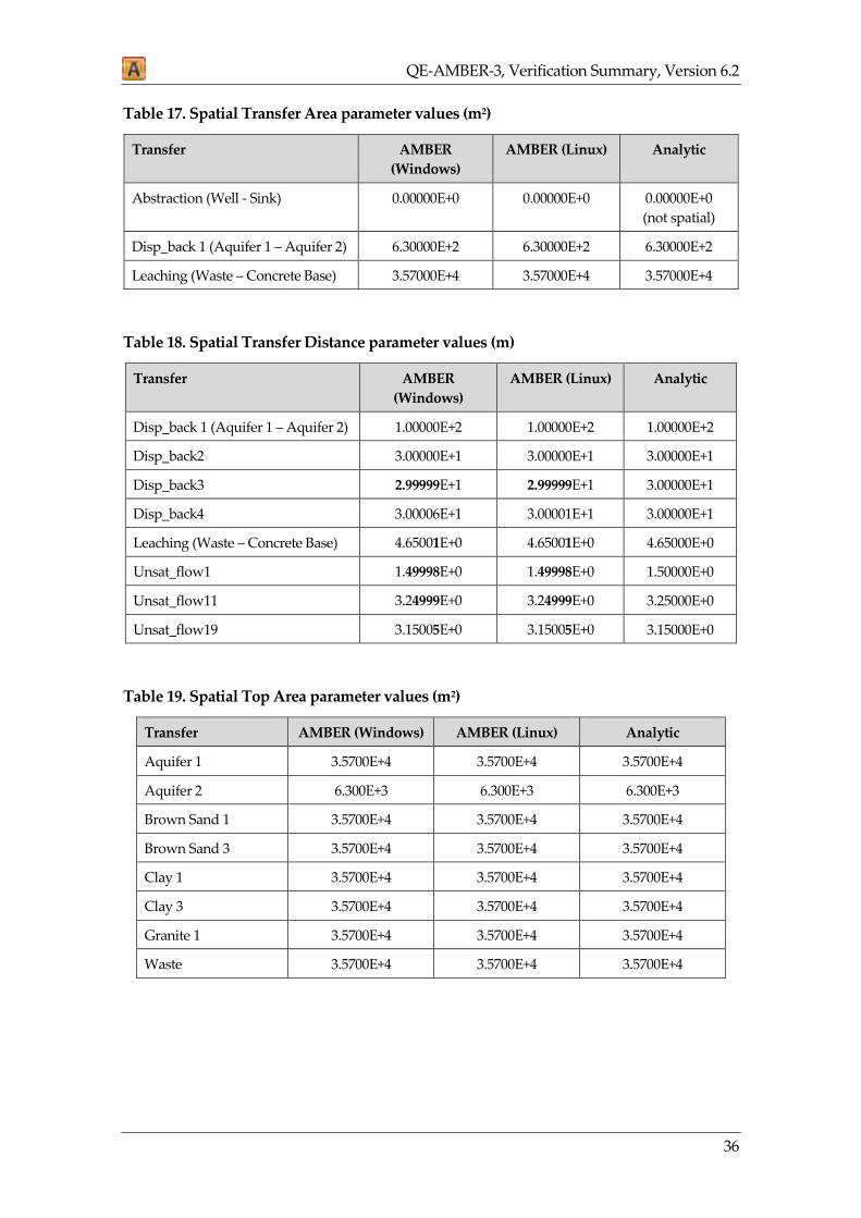
Table 17. Spatial Transfer Area parameter values (m2)

Transfer AMBER

(Windows)

AMBER (Linux) Analytic

Abstraction (Well - Sink) 0.00000E+0 0.00000E+0 0.00000E+0

(not spatial)

Disp_back 1 (Aquifer 1 – Aquifer 2) 6.30000E+2 6.30000E+2 6.30000E+2

Leaching (Waste – Concrete Base) 3.57000E+4 3.57000E+4 3.57000E+4

Table 18. Spatial Transfer Distance parameter values (m)

Transfer AMBER

(Windows)

AMBER (Linux) Analytic


Disp_back2 3.00000E+1 3.00000E+1 3.00000E+1

Disp_back3 2.99999E+1 2.99999E+1 3.00000E+1

Disp_back4 3.00006E+1 3.00001E+1 3.00000E+1


Unsat_flow1 1.49998E+0 1.49998E+0 1.50000E+0

Unsat_flow11 3.24999E+0 3.24999E+0 3.25000E+0

Unsat_flow19 3.15005E+0 3.15005E+0 3.15000E+0

Table 19. Spatial Top Area parameter values (m2)

Transfer AMBER (Windows) AMBER (Linux) Analytic

Aquifer 1 3.5700E+4 3.5700E+4 3.5700E+4

Aquifer 2 6.300E+3 6.300E+3 6.300E+3

Brown Sand 1 3.5700E+4 3.5700E+4 3.5700E+4

Brown Sand 3 3.5700E+4 3.5700E+4 3.5700E+4

Clay 1 3.5700E+4 3.5700E+4 3.5700E+4

Clay 3 3.5700E+4 3.5700E+4 3.5700E+4

Granite 1 3.5700E+4 3.5700E+4 3.5700E+4

Waste 3.5700E+4 3.5700E+4 3.5700E+4


37

Table 20. Spatial Donor Length parameter values (m)



Disp_back2 3.0E+1 3.0E+1 3.0E+1

Disp_back3 3.0E+1 3.0E+1 3.0E+1

Disp_back4 3.0E+1 3.0E+1 3.0E+1


Unsat_flow1 3E-1 3E-1 3E-1

Unsat_flow11 3.25E+0 3.25E+0 3.25E+0

Unsat_flow19 3..3E+0 3..3E+0 3.25E+0


38

10.2 Non-Cuboid Geometry

The three parameters were then tested for a simple spatial model with non-cuboid geometry,

shown in Figure 12. This test case is implemented in SpatialParameters.cse.

Figure 12. Simple non-cuboid geometry shown in the a) x-z and b) x-yplanes

The results from this model are compared with analytical solutions in Table 21 to Table 25.

There is good agreement within 5 significant figures.

Table 21. Spatial Volume parameter values (m3)

Compartment AMBER (Windows) AMBER (Linux) Analytic

Comp1 2.40000E+3 2.40000E+3 2.40000E+3

Comp2 8.00000E+3 8.00000E+3 8.00000E+3

Comp3 1.20000E+3 1.20000E+3 1.20000E+3

Comp4 1.20000E+3 1.20000E+3 1.20000E+3


39

Table 22. Spatial Transfer Area parameter values (m2)


Comp1_TO_Comp2 4.30813E+2 4.30813E+2 4.30813E+2

Comp2_TO_Comp3 2.23607E+2 2.23607E+2 2.23607E+2

Comp3_TO_Comp4 2.00000E+2 2.00000E+2 2.00000E+2

Table 23. Spatial Transfer Distance parameter values (m)


Comp1_TO_Comp2 1.24829E+1 1.24829E+1 1.24829E+1

Comp1_TO_Comp3 1.24828E+1 1.24828E+1 1.24829E+1

Comp3_TO_Comp4 7.33336E+00 7.33336E+00 7.33333E+00

Table 24. Spatial Top Area parameter values (m2)


Comp1 1.2000E+2 1.2000E+2 1.2000E+2

Comp2 4.0000E+2 4.0000E+2 4.0000E+2

Comp3 1.2000E+2 1.2000E+2 1.2000E+2

Comp4 2.56125E+2 2.56125E+2 2.56125E+2

Table 25. Spatial Donor Length parameter values (m)


Comp1_TO_Comp2 5.57086E+1 5.57086E+1 5.57086E+1

Comp1_TO_Comp3 3.71391E+1 3.71391E+1 3.71391E+1

Comp3_TO_Comp4 6.0000E+0 6.0000E+0 6.0000E+0

Note that the SpatialDonorLength is verified as donor volume divided by the interface area.


40

11 AMBER 6.2 Targeted Tests

In order to test the new functionalities added for AMBER 6.2, a series of pass/fail tests were

devised, based on the AMBER 6.2 Release Notes (Quintessa, 2017c). These tests have been

grouped together based on the functionalities tested below. All tests were passed in both

Windows and Linux operating systems.

11.1 Basic Parameter Functionality

The following tests relate to general parameter functionality.

New Internal Parameters: Check that new internal parameters, KgToBq and BqToKg

perform the unit conversions correctly.

Renaming Parameters: Standard and derived parameters with no multiplicity can be

renamed.

Parameter name validity checking: If a parameter name has any spaces in it they are

automatically replaced by “_”. For other illegal characters, a warning message appears

before changes are made to make the name acceptable in AMBER.

Renaming a parameter used elsewhere: The validity of the revised parameter name is

checked before a message asking if you would like to update expressions that use that

parameter.

Non-alphanumeric characters, spaces and hyphens not allowed in NameSet items:

Check is it not possible to use illegal characters in NameSet items or in the name of the

NameSet itself.

Self-Referable parameters: These parameters list themselves in the “Uses” and “Used

By” lists.

Internal Editable parameters only having value be changed: Check that all non-

editable aspects of internal editable parameters are greyed out and cannot be modified.

Donor/Receptor Mappings for Transfers: Check that when new transfers are added to

a model that the Donor/Receptor mappings are correctly updated.

11.2 GUI Properties and Functionality

Ability to export model window and spatial view as images: Check that the model

window for both the main model view and submodel views can be exported as each of

the different image types (png, gif, jpg, bmp, svg). Check that the 3D spatial view can be

exported as each of the different image types (png, gif, jpg, bmp). Note that this feature

is currently limited to export only the visible area of the 3D view.

Use of Tab and Shift+Tab to navigate a parameter grid: It is now possible to use Tab

and Shift+Tab to navigate right and left, respectively, in the grid of a parameter with

double multiplicity.


41

Right-Click Delete Option: Check that when a compartment, transfer or submodel is

right-clicked that ‘Delete’ appears as an option, and works.

Shortcut to Examples folder: There is now a shortcut under the File menu which opens

the folder with the AMBER example case files in it.

Copy+Paste Lookup Time Dependent Parameters: Check that when copying and

pasting a lookup time dependent parameter that the copied parameter is as expected.

Improved Error Messages: When the user attempts something that is not possible, the

error messages give more helpful information to resolve the issue encountered.

Warning before deleting Submodels: Check that if an attempt is made to delete a non-

empty submodel that an appropriate warning message appears.

11.3 Calculation and Output Tests

Multiple Outputs to Excel: When a graph is drawn and the “Output to Excel” option is

selected, this is remembered for subsequent graphs drawn in that session.

Running calculation once an error in case file fixed: If a case has failed to calculate due

to an error, then the error is fixed so it can calculate and you go to calculate again, then

there should be no warning regarding the ADF file as none would have been created

during the failed calculation.

11.4 Other Tests

Rename ‘Shape Preview’ to ‘3D View’.

Excel Graph Output: Ensure that all data is exported when plotting results in Excel.

Truncated Gaussian distribution: Ensure properties are all shown as expected.

Moving compartments: Moving compartments, and submodels, around in the Model

view tab no longer causes a crash.


42

12 Conclusions

The wide-ranging set of test cases documented here verifies the correct functioning of

AMBER 6.2 in both deterministic and probabilistic modes.

These, together with the extensive user interface testing conducted for AMBER 6.2 and the

continuous testing that the software undergoes when it is applied to new cases, show that the

code works well over a wide range of problem types.

Of course, no testing can rule out the possibility of there being undiscovered errors in the

code. To help find these, all users should report any incorrect, or suspicious, behaviour so

that it can be investigated and, if necessary, corrected in subsequent versions.

AMBER Support Team:

e-mail: [email protected]

Telephone: +44 (0)1925 885956

Address: Quintessa Limited,

The Hub,

14 Station Road,

Henley-on-Thames,

Oxfordshire RG9 1AY,

United Kingdom.

Website: https://www.quintessa.org/amber

References

ANDRA (2003). BIOSCOMP Project: Intercomparison Exercise between AQUABIOS,

AMBER and MEPAS for the Calculation of the Transfers of Non-Radioactive Pollutants

within the Biosphere. ANDRA Report Z RP 0ANT 03-029, December 2003.

BIOMOVS II (1996a). Validation Test for Carbon-14 Migration and Accumulation in a

Canadian Shield Lake. BIOMOVS II Technical Report No. 14, published on behalf of the

BIOMOVS II Steering Committee by the Swedish Radiation Protection Institute, Sweden.

BIOMOVS II (1996b). Biosphere Modelling for Dose Assessments of Radioactive Waste

Repositories: Final Report of the Complementary Studies Group. BIOMOVS II Technical

Report No. 12, published on behalf of the BIOMOVS II Steering Committee by the Swedish

Radiation Protection Institute, Sweden.

BIOMOVS II (1996c). Model Validation Studies of Water Flow and Radionuclide Transport

in Vegetated Soils Using Lysimeter Data. BIOMOVS II Technical Report No. 15, published

on behalf of the BIOMOVS II Steering Committee by the Swedish Radiation Protection

Institute, Sweden.

mailto:[email protected]

https://www.quintessa.org/amber


43

Côme B, Béon O, Albrecht A, Gallerand M O, Little R H and Strenge D L (2004). Evaluating

Multimedia Exposure Codes: the BIOSCOMP Exercise. In: Whelan G (ed.), Brownfields

Multimedia Modelling and Assessment, WIT Press, Southampton, UK.

IAEA (2003a). Improvement of Safety Assessment Methodologies for Near Surface Disposal

Facilities, Results of a co-ordinated research project. Volume II: Test Cases. International

Atomic Energy Agency, Vienna.

IAEA (2003b). “Reference Biospheres” for Solid Radioactive Waste Disposal: Report of

BIOMASS Theme 1 of the BIOsphere Modelling and ASSessment (BIOMASS) Programme.

IAEA-BIOMASS-6, International Atomic Energy Agency, Vienna.

IAEA (2003c). The Use of Safety Assessment in the Derivation of Activity Limits for Disposal

of Radioactive Waste to Near Surface Facilities. IAEA-TECDOC-1380, International Atomic

Energy Agency, Vienna.

Jones J, Vahlund F, Kautsky U and Kärnbränslehantering S (2004). Tensit – a Novel

Probabilistic Simulation Tool for Safety Assessments: Tests and Verifications Using

Biosphere Models. SKB Technical Report TR-04-07, June 2004.

Maul P R and Robinson P C (2002). Exploration of Important Issues for the Safety of SFR 1

using Performance Assessment Calculations, SKI Report 02:62, June 2002.

Maul P R, Robinson P C, Broed R, and Avila R (2004). Further AMBER and Ecolego

Intercomparisons. SKI Report 2004:05/SSI Report 2004:01, Stockholm, January 2004.

Maul P R, Robinson P C, Avila R, Broed R, Pereira A and Xu S (2003). AMBER and Ecolego

Intercomparisons using Calculations from SR 97. SKI Report 2003:28/SSI Report 2003:11,

Stockholm, August 2003.

NEA (1993). PSACOIN Level 1B Intercomparison, edited by R.A.Klos et al, OECD, Paris;

1993.

Penfold J (2014). Further Reproduction of SKB’s Calculation Cases and Independent

Calculations of Additional “What If” Cases. Strålsäkerhetsmyndigheten (SSM) Technical

Note 2014:55, Stockholm, Sweden.

Quintessa (2017a). AMBER 6.2 Reference Manual. Quintessa Limited report QE-AMBER-1,

Version 6.2, Henley-on-Thames, UK.

Quintessa (2017b). AMBER 6.2 User Guide. Quintessa Limited report QE-AMBER-2,

Version 6.2, Henley-on-Thames, UK.

Quintessa (2017c). AMBER 6.2 Release Note. Quintessa Limited technical note

QE-AMBER-M4, Version 6.2, Henley-on-Thames, UK.

Robinson, P C, Hodgkinson D P, Tasker P W, Lever D A, Windsor M E, Grime P W and

Herbert A W (1988). A solubility-limited source-term model for the geological disposal of

cemented intermediate-level waste. UKAEA Report R-11854; BNFL Report ILWRP/87/P.12;

DOE Report DOE/RW/88.015; 1988.


44

Scott F A M (1998). An Investigation into the Application of Compartmental Models in their

Representation of Contaminants in the Environment. MSc Thesis, Centre for Environmental

Technology, Imperial College of Science, Technology and Medicine, University of London.

Towler G, Watson C, Maul P and Robinson P (2014). Review of Radionuclide Transport in

the Posive Safety Case for Olkiluoto. Quintessa Limited report QRS-1664E-1, V1.0.

Walke R C (2014). Modelling Comparison of Simple Reference Biosphere Models with LDF

Models. Strålsäkerhetsmyndigheten (SSM) Technical Note 2014:34, Stockholm, Sweden.

Walke R C and Limer L M C (2014). Further Modelling Comparison of Simple Reference

Biosphere Models with the LDF Modelling Approach. Strålsäkerhetsmyndigheten (SSM)

Technical Note 2014:54, Stockholm, Sweden.

Walke R C, Kirchner G, Xu S and Dverstorp B (2015). Post-closure biosphere assessment

modelling: comparison of complex and more stylised approaches. Journal of Environmental

Radioactivity 148, pp. 50-58.

Watkins B M, Robinson P C, Smith G M (1998). Update of Models for Assessing Short-Term

Atmospheric Releases of C-14 and Tritium in the Light of New Information and Experimental

Data. QuantiSci Report to the Ministry of Agriculture, Fisheries and Food, MAFF-5044-1,

version 1.0, QuantiSci Ltd, Henley-on-Thames, UK.

Williams M J and Woods J A (1994). Technical Description of the SPADE Solver for

Differential and Algebraic Equations. QuantiSci Report IENV-COD/12-1, version 1.0,

QuantiSci Ltd, Henley-on-Thames, UK.

amber 6.2 verification summary - quintessa limited verification... · qe-amber-3, verification...

Documents