AM205: Assignment 3 solutions∗

Problem 1 – convergence rates of two integrals

Part (a)

As discussed in class, the trapezoidal integration method has the form

IA ≈ h(

12

f (x0) + f (x1) + f (x2) + ... + f (xn−1) +12

f (xn)

). (1)

To compute the error bound, we need to calculate the second derivative of f . We have

d2 fdx2 =

cos x(54 − cos x)2 − 2 sin2 x(5

4 − cos x)(5

4 − cos x)4. (2)

The left panel of Fig. 1 shows the error bound and error versus h on a log–log scale. Theerror bound is always larger than the error. In addition, the slope of error versus h is 2,which verifies that the trapezoidal method is second-order accurate.

Part (b)

This part is analogous to part (a), except that the error decays exponentially with h. In thiscase, we observe trapezoidal method has exponential convergence (faster than O(hm) forany m). This is due to a special property of the trapezoidal rule when evaluating periodicintegrals. The right panel of Fig. 1 shows the error bound and error versus h on a log–logscale.

Part (c)

Here, we show that

IB =∫ 2π

0f (x)dx =

∫ 2π

0

dx54 − cos x

=8π

3(3)

using the residue theorem. If z = eiθ then cos θ = z+z−1

2 . The denominator of the integralin Eq. 3 can be rewritten as

54− cos θ =

54− z + z−1

2=

54− z2 + 1

2z=−z2 + 2az− 1

2z. (4)

Substituting this expression into the integral transforms it to∮C

1i

2dzz2 − 5

2 z + 1, (5)

∗Solutions to problems 1, 2, and 4 were written by Kevin Chen. Solutions to problems 3, 5 and 6 werewritten by Chris H. Rycroft. Edited by Chris H. Rycroft.

1

10−2

10−1

100

101

10−5

10−4

10−3

10−2

10−1

100

101

h

erro

r

trap errorerror bound

10−2

10−1

100

101

10−14

10−12

10−10

10−8

10−6

10−4

10−2

100

102

h

erro

r

trap errorerror bound

Figure 1: Errors and error bounds as a function of the integration step size h for the two integralsconsidered in problem 1. The left panel shows results for

∫ π/30 f (x)dx and the right panel shows

results for∫ 2π

0 f (x)dx.

where the closed contour C represents unit circle in the complex plane. The integrand hastwo poles at z = 2 and z = 1

2 , and only the pole inside the closed contour contributes tothe integral. Invoking the residual theorem yields the result

IB = 2πi Res

(1i

2dzz2 − 5

2 z + 1, z =

12

)=

8π

3. (6)

Problem 2 – adaptive integration

Part (a) – 3-point Gauss quadrature

The third Legendre polynomial is P3(x) = 12 x(5x2 − 3), which has roots at

x1 = −√

35

, x2 = 0, x3 =

√35

.

We now solve for the weights by integrating the Lagrange interpolation polynomialsthrough these three points. We have

w0 =∫ 1

−1Lo(x)dx =

∫ 1

−1

x− 0−√

3/5− 0× x−

√3/5

−√

3/5−√

3/5dx

=56

∫ 1

−1(x2 −

√3/5x)dx =

56

∫ 1

−1(x2)dx

=56

23=

59

. (7)

2

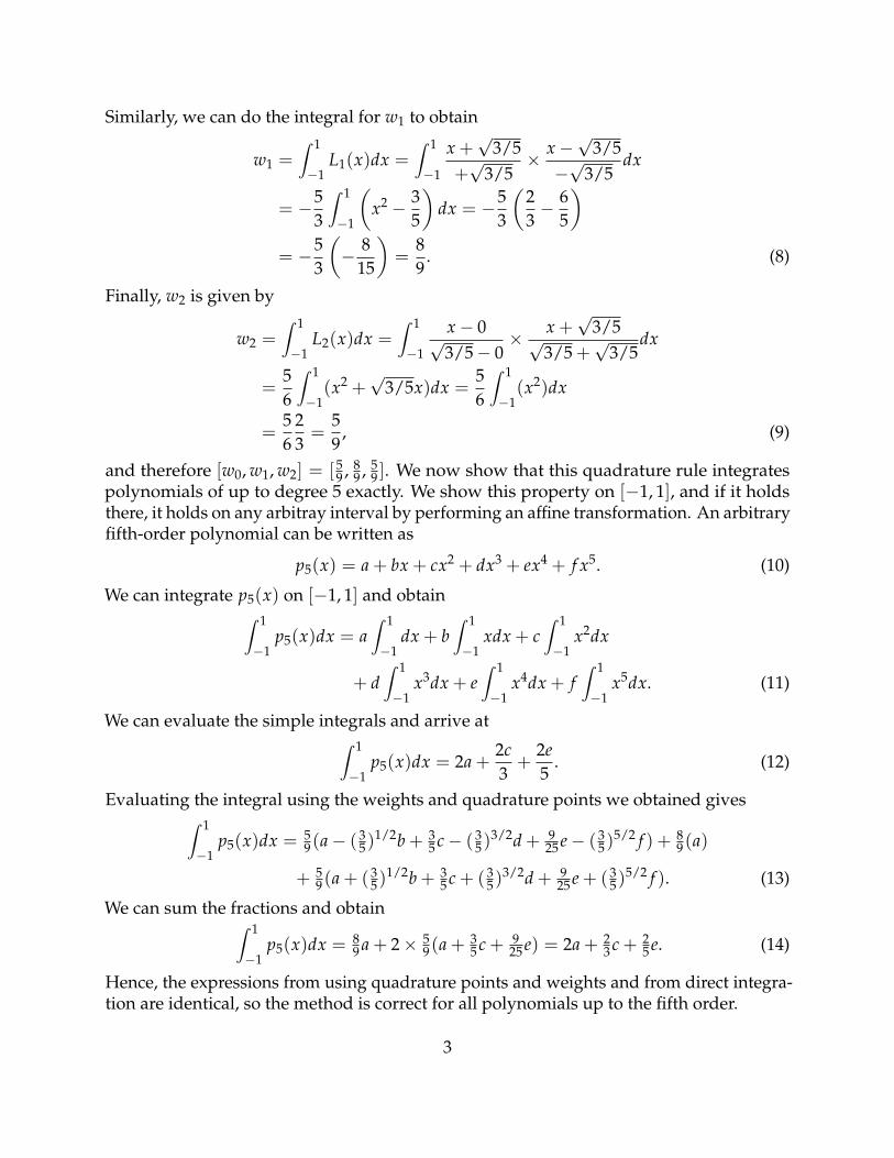
Similarly, we can do the integral for w1 to obtain

w1 =∫ 1

−1L1(x)dx =

∫ 1

−1

x +√

3/5+√

3/5× x−

√3/5

−√

3/5dx

= −53

∫ 1

−1

(x2 − 3

5

)dx = −5

3

(23− 6

5

)= −5

3

(− 8

15

)=

89

. (8)

Finally, w2 is given by

w2 =∫ 1

−1L2(x)dx =

∫ 1

−1

x− 0√3/5− 0

× x +√

3/5√3/5 +

√3/5

dx

=56

∫ 1

−1(x2 +

√3/5x)dx =

56

∫ 1

−1(x2)dx

=56

23=

59

, (9)

and therefore [w0, w1, w2] = [59 , 8

9 , 59 ]. We now show that this quadrature rule integrates

polynomials of up to degree 5 exactly. We show this property on [−1, 1], and if it holdsthere, it holds on any arbitray interval by performing an affine transformation. An arbitraryfifth-order polynomial can be written as

p5(x) = a + bx + cx2 + dx3 + ex4 + f x5. (10)

We can integrate p5(x) on [−1, 1] and obtain∫ 1

−1p5(x)dx = a

∫ 1

−1dx + b

∫ 1

−1xdx + c

∫ 1

−1x2dx

+ d∫ 1

−1x3dx + e

∫ 1

−1x4dx + f

∫ 1

−1x5dx. (11)

We can evaluate the simple integrals and arrive at∫ 1

−1p5(x)dx = 2a +

2c3+

2e5

. (12)

Evaluating the integral using the weights and quadrature points we obtained gives∫ 1

−1p5(x)dx = 5

9(a− (35)

1/2b + 35 c− (3

5)3/2d + 9

25 e− (35)

5/2 f ) + 89(a)

+ 59(a + (3

5)1/2b + 3

5 c + (35)

3/2d + 925 e + (3

5)5/2 f ). (13)

We can sum the fractions and obtain∫ 1

−1p5(x)dx = 8

9 a + 2× 59(a + 3

5 c + 925 e) = 2a + 2

3 c + 25 e. (14)

Hence, the expressions from using quadrature points and weights and from direct integra-tion are identical, so the method is correct for all polynomials up to the fifth order.

3

m Integral value Estimated error Num. of intervals4 2.07598 0 15 1.73474 2.22× 10−16 16 2.08968 3.92× 10−7 87 1.88568 5.98× 10−7 118 2.20458 2.93× 10−7 13

Table 1: Integral values, estimated error, and number of intervals for the 3-point adaptive Gaussquadrature scheme applied to the integral

∫ 5/4−1 (xm − x2 + 1)dx for various values of m.

Integral Integral value Estimated error Num. of intervals∫ 1−1 |x|dx 1 0 2∫ 2−1 |x|dx 2.50000 7.2055× 10−11 16∫ 1

0 x3/4 sin 1x dx 0.4070269 8.73296× 10−8 194326

Table 2: Integral values, estimated error, and number of intervals for four sample integrals, usingthe 3-point adaptive Gauss quadrature scheme.

Part (b) – adaptive integration through 3 point Gauss quadrature

We now implement the adaptive scheme using 3-point Gauss quadrature as discussed inpart (a)—see the attached code examples for details. For the integrals of the form∫ 5/4

−1(xm − x2 + 1)dx, (15)

the computed values, estimated error, and number of intervals are given in Table 1. Asexpected from part (a), the integrals for m = 4 and m = 5 are computed exactly with asingle integration step. The integrals for m ≥ 6 are determined to high accuracy with asmall number of subdivisions of the interval.

Part (c) – sample integrals

We use the same integration routine to compute the integrals given in this problem. Theanswers are tabulated in Table 2.

Problem 3 – integration of a family of functions

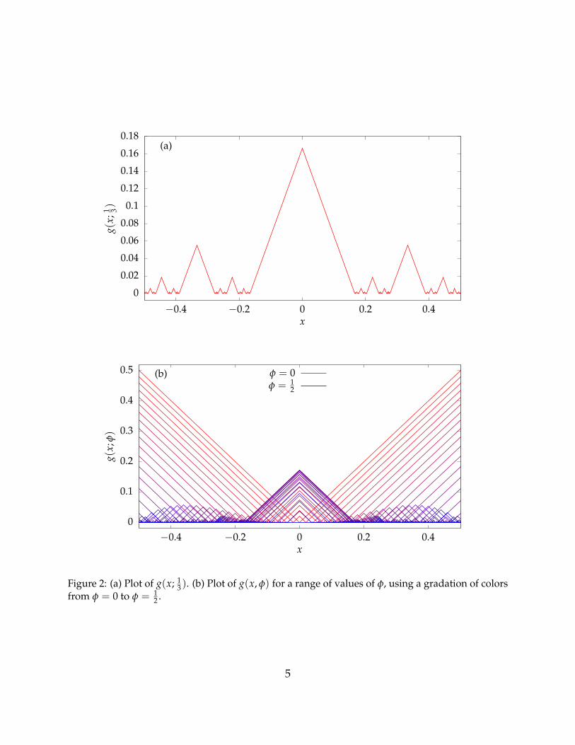
Figure 2(a) shows a plot of the function g(x; 13). The recursive construction of g results

in a function with many peaks in a fractal arrangement that is reminiscent of the Kochcurve.† Figure 2(b) shows a plot of g(x, φ) for twenty six different values of φ in the rangefrom 0 to 1

2 . For φ = 0, g(x; φ) = |x| since all of the φk terms vanish. For φ = 12 , the graph

†https://en.wikipedia.org/wiki/Koch_snowflake

4

0

0.02

0.04

0.06

0.08

0.1

0.12

0.14

0.16

0.18

−0.4 −0.2 0 0.2 0.4

(a)

g(x;

1 3)

x

0

0.1

0.2

0.3

0.4

0.5

−0.4 −0.2 0 0.2 0.4

(b)

g(x;

φ)

x

φ = 0φ = 1

2

Figure 2: (a) Plot of g(x; 13 ). (b) Plot of g(x, φ) for a range of values of φ, using a gradation of colors

from φ = 0 to φ = 12 .

5

0

0.05

0.1

0.15

0.2

0.25

0 0.2 0.4 0.6 0.8 1

(a)

0

500

1000

1500

2000

2500

3000

3500

4000

4500

0 0.2 0.4 0.6 0.8 1

(b)

Inte

gral

valu

e

φ

Num

ber

ofin

terv

als

φ

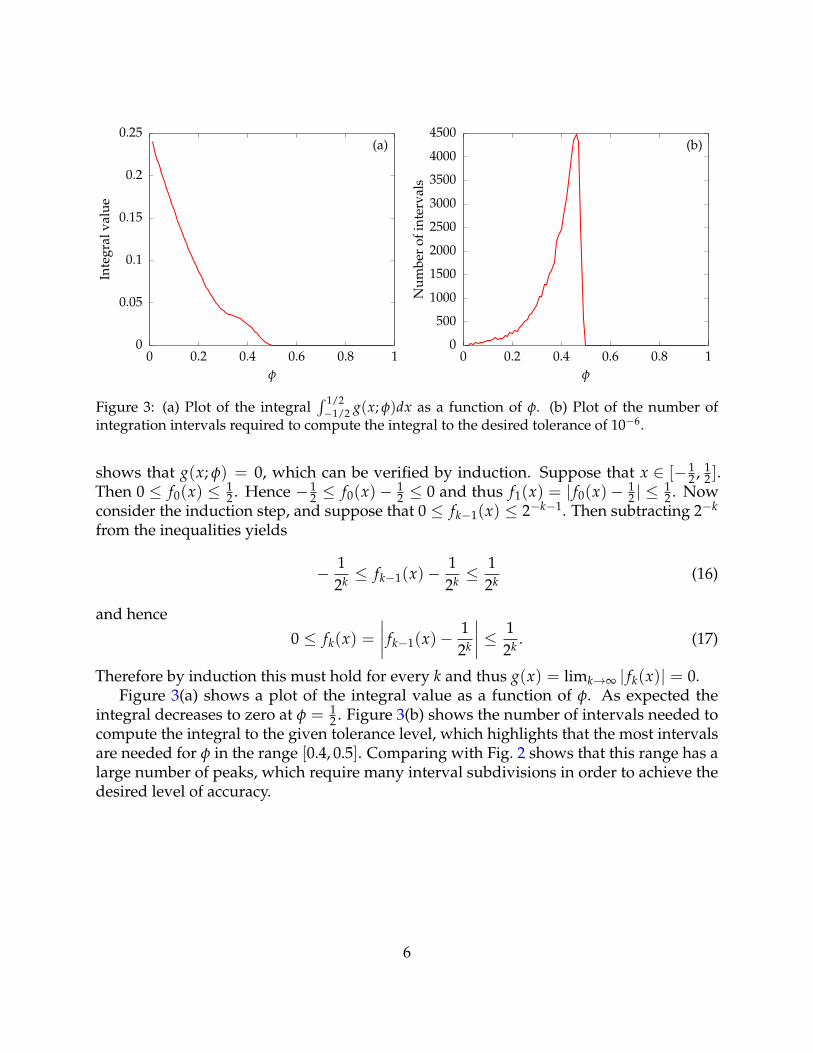
Figure 3: (a) Plot of the integral∫ 1/2−1/2 g(x; φ)dx as a function of φ. (b) Plot of the number of

integration intervals required to compute the integral to the desired tolerance of 10−6.

shows that g(x; φ) = 0, which can be verified by induction. Suppose that x ∈ [−12 , 1

2 ].Then 0 ≤ f0(x) ≤ 1

2 . Hence −12 ≤ f0(x)− 1

2 ≤ 0 and thus f1(x) = | f0(x)− 12 | ≤

12 . Now

consider the induction step, and suppose that 0 ≤ fk−1(x) ≤ 2−k−1. Then subtracting 2−k

from the inequalities yields

− 12k ≤ fk−1(x)− 1

2k ≤12k (16)

and hence

0 ≤ fk(x) =∣∣∣∣ fk−1(x)− 1

2k

∣∣∣∣ ≤ 12k . (17)

Therefore by induction this must hold for every k and thus g(x) = limk→∞ | fk(x)| = 0.Figure 3(a) shows a plot of the integral value as a function of φ. As expected the

integral decreases to zero at φ = 12 . Figure 3(b) shows the number of intervals needed to

compute the integral to the given tolerance level, which highlights that the most intervalsare needed for φ in the range [0.4, 0.5]. Comparing with Fig. 2 shows that this range has alarge number of peaks, which require many interval subdivisions in order to achieve thedesired level of accuracy.

6

Problem 4 – error analysis of a numerical integration rule

Part (a)

We want to use Taylor series to prove the midpoint method

yk+1 = yk + h f(

tk+1/2,yk + yk+1

2

)(18)

converges as a function of h2, where h = tk+1 − tk. We expand y(tk+1) and y(tk) aroundtk+1/2 and obtain

y(tk+1) = y(tk+1/2) +h2

y′(tk+1/2) +h2

8y′′(tk+1/2) + O(h3)y′′′(tk+1/2),

y(tk) = y(tk+1/2)−h2

y′(tk+1/2) +h2

8y′′(tk+1/2) + O(h3)y′′′(tk+1/2) (19)

We can arrive at

y(tk+1)− y(tk)

h= y′(tk+1/2) + O(h3)y′′′(tk+1/2). (20)

We can also expand f (tk+1/2, y(tk)+y(tk+1)2 ) around tk+1/2 and obtain

f(

tk+1/2, y(tk)+y(tk+1)2

)= f

(tk+1/2, y(tk+1/2) +

y(tk)+y(tk+1)2 − y(tk+1/2)

)= y′(tk+1/2) +

(y(tk) + y(tk+1)

2− y(tk+1/2)

)∂ f∂y

∣∣∣∣y(tk+1/2)

+ O(

y(tk) + y(tk+1)

2− y(tk+1/2)

)2 ∂2 f∂y2

∣∣∣∣y(tk+1/2)

. (21)

We can plug in the Taylor expansion of y(tk) and y(tk+1) around y(tk+1/2) to obtain

y(tk) + y(tk+1)

2− y(tk+1/2) =

h2

8y′′(tk+1/2) + O(h3)y′′′(tk+1/2). (22)

As a result, we arrive at the expression

f(

tk+1/2, y(tk)+y(tk+1)2

)= y′(tk+1/2) +

∂ f∂y

∣∣∣∣y(tk+1/2)

(h2

4y′′(tk+1/2) + O(h3)y′′′(tk+1/2)).

(23)Using Eqs. 20 and 23, we aim to compute the truncation error Tk, which gives the conver-gence rate of the method as we invoke the theorem discussed in lecture. The truncationerror is given by

Tk =y(tk+1)− y(tk)

h− f

(tk+1/2,

y(tk) + y(tk+1)

2

)(24)

7

and hence

Tk = y′(tk+1/2) + O(h3)y′′′(tk+1/2)− y′(tk+1/2)

− ∂ f∂y

∣∣∣∣y(tk+1/2)

(h2

4y′′(tk+1/2) + O(h3)y′′′(tk+1/2)

). (25)

Therefore Tk is O(h2) and the method is second-order accurate.

Stability region of midpoint method

We want to find the stability region of the midpoint method for the ode y′ = λy. We plugthe differential equation into the midpoint method and obtain

yk+1 = yk + hλ

(yk + yk+1

2

). (26)

Rearranging the equation leads to

yk+1

(1− hλ

2

)= yk

(1 +

hλ

2

), (27)

which can be rewritten as

yk+1 =

(1 + h/21− h/2

)yk, (28)

where h = hλ ∈ C. This equation is stable if and only if∣∣∣∣1 + h/21− h/2

∣∣∣∣ ≤ 1. (29)

If h is written in terms of real and imaginary parts as h = a + ib then(1 + a

2

)2+ b2 ≤

(1− a

2

)2+ b2 (30)

and hencea ≤ −a, (31)

which implies a ≤ 0 and b ∈ R. Hence, the asymptotically stable case is when h isthe imaginary axis. Anywhere left of the imaginary axis gives strictly converging case.Hence, to have convergence, the discretization of the differential equation must satisfy theRe h ≤ 0. Figure 4 shows the stability region.

8

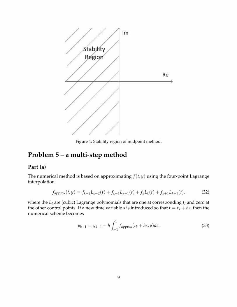
Figure 4: Stability region of midpoint method.

Problem 5 – a multi-step method

Part (a)

The numerical method is based on approximating f (t, y) using the four-point Lagrangeinterpolation

fapprox(t, y) = fk−2Lk−2(t) + fk−1Lk−1(t) + fkLk(t) + fk+1Lk+1(t). (32)

where the Ll are (cubic) Lagrange polynomials that are one at corresponding tl and zero atthe other control points. If a new time variable s is introduced so that t = tk + hs, then thenumerical scheme becomes

yk+1 = yk−1 + h∫ 1

−1fapprox(tk + hs, y)ds. (33)

9

To proceed, consider the integrals of the Lagrange polynomials:∫ 1

−1Lk−2(tk + hs)ds =

1−6

∫ 1

−1(s− 1)s(s + 1)ds = 0, (34)∫ 1

−1Lk−1(tk + hs)ds =

12

∫ 1

−1(s− 1)s(s + 2)ds =

13

, (35)∫ 1

−1Lk(tk + hs)ds =

1−2

∫ 1

−1(s− 1)(s + 1)(s + 2)ds =

43

, (36)∫ 1

−1Lk+1(tk + hs)ds =

16

∫ 1

−1s(s + 1)(s + 2)ds =

13

. (37)

Note that the integral of Lk−2 vanishes because of symmetry. This is an advantage, since itensures that the numerical scheme will achieve a higher order of accuracy, with one fewerfunction evaluation. Hence Eq. 33 becomes

yk+1 = yk−1 +h3( fk−1 + 4 fk + fk+1) . (38)

Part (b)

To solve the differential equation

y′′(t) + 2y′(t) + 17y(t) = 0. (39)

with initial conditions y(0) = 1, y′(0) = 0, consider a possible solution of y = emt. To be asolution, the parameter m must satisfy

m2 + 2m + 17 = 0, (40)

which can also be written as(m + 1)2 = −16. (41)

This has two solutions, m = −1± 4i. Hence, the general solution has the form

y(t) = e−t(A cos 4t + B sin 4t) (42)

where A and B are constants. The first derivative is

y′(t) = e−t((4B− A) cos 4t− (4A + B) sin 4t) (43)

and hencey(0) = A, y′(0) = 4B− A. (44)

Hence A = 1 and B = 14 to satisfy the initial conditions.

10

−0.6

−0.4

−0.2

0

0.2

0.4

0.6

0.8

1

0 0.5 1 1.5 2 2.5 3

y(t)

t

ExactNumerical

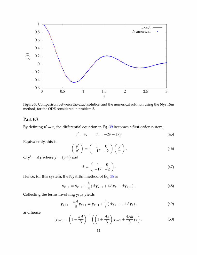
Figure 5: Comparison between the exact solution and the numerical solution using the Nystrommethod, for the ODE considered in problem 5.

Part (c)

By defining y′ = v, the differential equation in Eq. 39 becomes a first-order system,

y′ = v, v′ = −2v− 17y (45)

Equivalently, this is (y′

v′

)=

(1 0−17 −2

)(yv

), (46)

or y′ = Ay where y = (y, v) and

A =

(1 0−17 −2

). (47)

Hence, for this system, the Nystrom method of Eq. 38 is

yk+1 = yk−1 +h3(Ayk−1 + 4Ayk + Ayk+1) . (48)

Collecting the terms involving yk+1 yields

yk+1 −hA3

yk+1 = yk−1 +h3(Ayk−1 + 4Ayk) , (49)

and hence

yk+1 =

(1− hA

3

)−1 ((1 +

Ah3

)yk−1 +

4Ah3

yk

). (50)

11

10−16

10−14

10−12

10−10

10−8

10−6

10−4

10−2

10−3 3× 10−3 0.01 0.03 0.1

Abs

olut

eer

ror

Step size h

Exact set-upLinear fit

Euler set-upLinear fit

Figure 6: Graph showing the absolute error between the exact and numerical solutions at t = 3 afunction of the step size h, for the ODE considered in problem 5. The graph shows the absoluteerrors for the case when the first two steps are set using the exact solution, and for the case whenthey are set using Euler steps. In each case a line of best fit, fitted over the range 10−3 ≤ h ≤ 10−2,is shown.

This is now an explicit formula for yk+1 in terms of the previous values of y. The programq5.py implements this numerical scheme. Figure shows the exact and numerical solutionsand demonstrates that they are near-identical.

Figure 6 shows a log–log plot of the absolute error between the exact and numerical yfor a variety of step sizes between h = 10−1 and h = 10−3. The plot also contains a line ofbest fit, which has a slope of 3.995, confirming that the method is fourth-order accurate.It is worth noting that the method is a remarkably efficient way to achieve fourth-orderaccuracy, since it only requires considering the previous two values at each step.

Part (d)

Figure 6 also shows the absolute error between the exact and numerical solutions when y1and y2 are set using an Euler step. Second-order accuracy is observed, with the best-fitline having slope of 2.009. This should be expected since the truncation error of the Eulermethod is O(h). Since two steps of size h are taken to determine y1 and y2, the local errorincurred is O(h2). The error on these first two steps will dominate the global error at t = 3.

12

Problem 6 – asteroid collision

Part (a)

The Jacobi integral is

J(x, y, u, v) = (x + µ)2 + y2 +2(1− µ)√

x2 + y2+

2µ√(x− 1)2 + y2

− u2 − v2. (51)

The asteroid’s equations of motion are given by the partial derivatives of J,

x′ = u,

y′ = v,

u′ = v + (x− µ)− (1− µ)x(x2 + y2)3/2 −

µ(x− 1)((x− 1)2 + y2)3/2 ,

v′ = −u + y− (1− µ)y(x2 + y2)3/2 −

µy((x− 1)2 + y2)3/2 . (52)

Part (b)

Consider a line segment between two points x1 and x2, and define ∆x = x2 − x1. Considerthe infinite line

x = x1 + λ∆x (53)

where λ ∈ R. The value of λ that minimizes the distance of x from the origin is given byprojecting out part of x1 in the direction of ∆x. This is given in terms of scalar products as

λ = − x1 · ∆x∆x · ∆x

. (54)

If λ ∈ [0, 1], then this point will on the line segment between x1 and x2. If λ < 0, then theclosest point on the segment to the origin will be x1. If λ > 1, then the closest point on thesegment to the origin will be x2.

Define this closest point is xmin. If |xmin| < R then the line segment intersects the circleof radius R at the origin. Otherwise, it does not intersect. This calculation is incorporated inthe detect function in the program threebody.py that is used in the subsequent sections.

Parts (c) and (d)

If the trajectory is assumed to be linear from t = 0 to t = 0.02, then the velocity at t = 0 is

v(0) =x(0.02)− x(0)

0.02. (55)

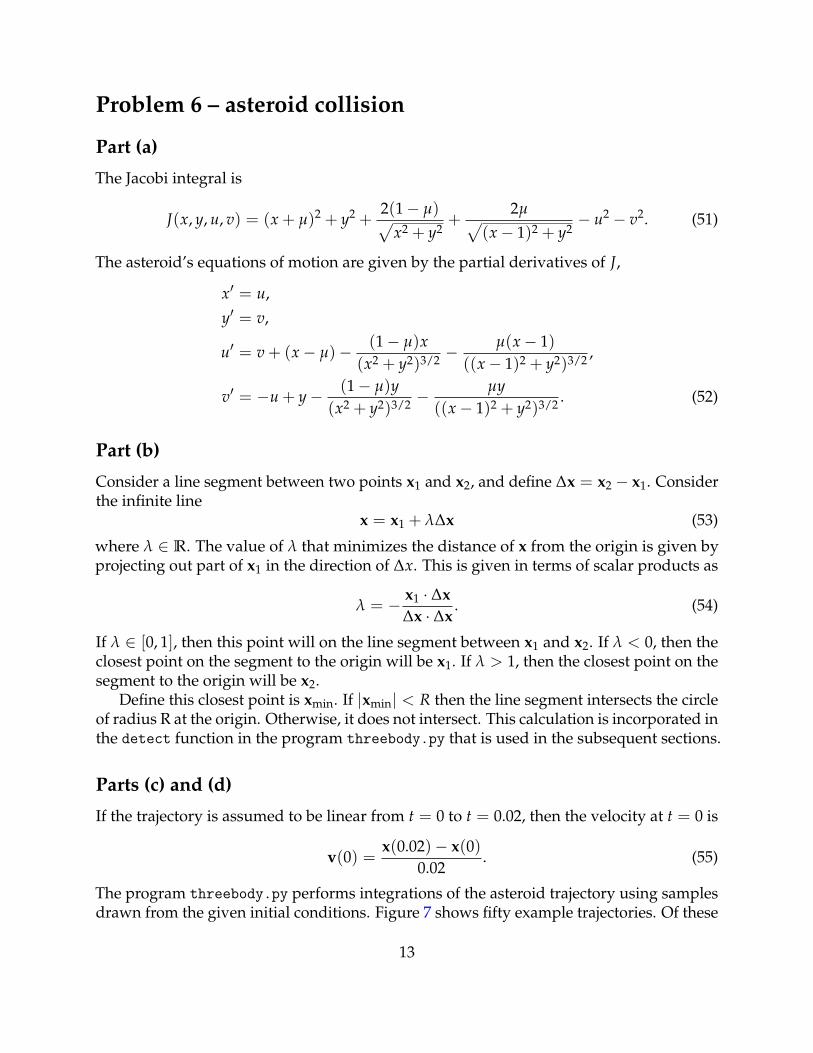
The program threebody.py performs integrations of the asteroid trajectory using samplesdrawn from the given initial conditions. Figure 7 shows fifty example trajectories. Of these

13

−1

−0.5

0

0.5

1

−1 −0.5 0 0.5 1 1.5 2

y

xFigure 7: Fifty possible asteroid trajectories. The Earth is the circle at the origin, and the Moon isthe circle at (1, 0).

−1

−0.5

0

0.5

1

−1 −0.5 0 0.5 1 1.5 2

(a)

−1 −0.5 0 0.5 1 1.5 2

(b)

y

x x

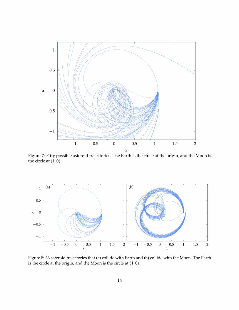
Figure 8: 36 asteroid trajectories that (a) collide with Earth and (b) collide with the Moon. The Earthis the circle at the origin, and the Moon is the circle at (1, 0).

14

Type Cases (linear) Percent SE Cases (exact) Percent SEEscape, t ∈ [0, 10] 338,440,422 67.69 0.0021 346,954,316 69.39 0.0021Earth, t ∈ [0, 10] 128,014,461 25.60 0.0020 118,983,556 23.80 0.0019Moon, t ∈ [0, 10] 939,012 0.1878 0.00019 942,510 0.1885 0.00019Escape, t ∈ (10, 200] 32,457,022 6.491 0.0011 32,968,484 6.594 0.0011Earth, t ∈ (10, 200] 42,920 0.008584 4.1× 10−5 46,508 0.009302 4.3× 10−5

Moon, t ∈ (10, 200] 52,035 0.01041 4.6× 10−5 52,782 0.01056 4.6× 10−5

Persistent, t > 200 54,128 0.01083 4.7× 10−5 51,844 0.01037 4.6× 10−5

Total 500,000,000 100 0 500,000,000 100 0

Table 3: Total occurrences of each type of trajectory, based on two sets of 500× 108 trials. Columns 2–4 contain results for when the asteroid velocity is assumed to be linear between the two observations,and columns 5–7 contain results for when the asteroid velocity is precisely fit so that the trajectorygoes through the two observations. For each set of results, the probability of each type of trajectoryis reported, along with a measure of standard error (SE) of the measurement. The SE is calculatedby assuming the counts follow a binomial distribution.

fifty trajectories, the majority quickly escape the Earth–Moon system, suggesting that thisis the most likely scenario.

Figure 8(a) shows 36 trajectories that collide with the Earth. All but one of the trajec-tories collides with the Earth after a single arc. However, a single trajectory collides byfirst orbiting around the Moon, demonstrating the possibility of complex interactions inthe three-body system. Figure 8(b) shows 36 trajectories that collide with the Moon. Themajority undergo several close passes around the Earth, before colliding with the Moon.

Table 3 shows the estimated probabilities of the different scenarios, based on 5× 108

trials. A trajectory is classified as escaping the Earth–Moon system if |x| > 20. This doesnot rigorously guarantee that a trajectory will escape, but in practice it is a very goodindication. Over the interval t ∈ [0, 10], one finds that 67.69% of trajectories escape, 25.60%of trajectories collide with the Earth, and 0.1878% of trajectories collide with the Moon.The remaining 6.521% of trajectories persist until t = 10, and are analyzed in more detailin part (f).

Part (e)

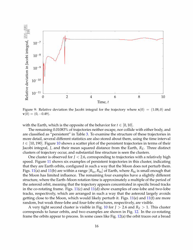
Figure 9 shows a plot of the relative deviation in the Jacobi integral over the time intervalfrom 0 to 10 for the given initial conditions. The relative deviation remains smaller than10−6 throughout the calculation.

Part (f)

For any trajectory that persists until t = 10, the threebody.py program performs a secondintegration up to t = 200. Over this extended time window, 6.491% escape, 0.008584%collide with the Earth, and 0.01041% collide with the Moon. Interestingly, over thisextended time window the probability of colliding with the Moon is higher than colliding

15

10−11

10−10

10−9

10−8

10−7

0 2 4 6 8 10

Rel

ativ

ede

viat

ion

inJa

cobi

inte

gral

,|J(

t)−

J(0)|

J(0)

Time, t

Figure 9: Relative deviation the Jacobi integral for the trajectory where x(0) = (1.08, 0) andv(0) = (0,−0.49).

with the Earth, which is the opposite of the behavior for t ∈ [0, 10].The remaining 0.01083% of trajectories neither escape, nor collide with either body, and

are classified as “persistent” in Table 3. To examine the structure of these trajectories inmore detail, several different statistics are also stored about them, using the time intervalt ∈ [10, 190]. Figure 10 shows a scatter plot of the persistent trajectories in terms of theirJacobi integral, J, and their mean squared distance from the Earth, RE. Three distinctclusters of trajectory occur, and substantial fine structure is seen the clusters.

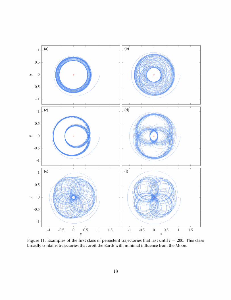
One cluster is observed for J < 2.6, corresponding to trajectories with a relatively highspeed. Figure 11 shows six examples of persistent trajectories in this cluster, indicatingthat they are Earth orbits, configured in such a way that the Moon does not perturb them.Figs. 11(a) and 11(b) are within a range [Rlo, Rhi] of Earth, where Rhi is small enough thatthe Moon has limited influence. The remaining four examples have a slightly differentstructure, where the Earth–Moon rotation time is approximately a multiple of the period ofthe asteroid orbit, meaning that the trajectory appears concentrated in specific broad tracksin the co-rotating frame. Figs. 11(c) and 11(d) show examples of one-lobe and two-lobetracks, respectively, which are arranged in such a way that the asteroid largely avoidsgetting close to the Moon, which would likely perturb it. Figs. 11(e) and 11(f) are morerandom, but weak three-lobe and four-lobe structures, respectively, are visible.

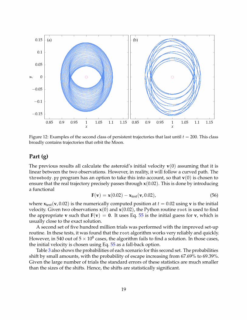
A very tight second cluster is visible in Fig. 10 for J > 2.6 and RE > 1. This clustercorresponds to lunar orbits, and two examples are shown in Fig. 12. In the co-rotatingframe the orbits appear to precess. In some cases like Fig. 12(a) the orbit traces out a broad

16

1.4

1.6

1.8

2

2.2

2.4

2.6

2.8

3

3.2

0.5 0.55 0.6 0.65 0.7 0.75 0.8 0.85 0.9 0.95 1 1.05

Jaco

biin

tegr

al,J

Root mean squared distance from Earth, RE

Figure 10: Scatter plot showing all of the asteroid trajectories that persist until t = 200, arrangedaccording to their Jacobi integral and root mean squared distance from Earth. 54,128 trajectories areshown, out of the total of 500× 108 that were simulated.

swath of space in the co-rotating frame, but in others like Fig. 12(b) the orbit appearslocked into a small number of distinct tracks. It is not clear whether Fig. 12(b) is purelycoincidental or if resonances due to the Earth cause this behavior.

The final cluster visible in Fig. 10 has J > 2.6 and RE < 1 and corresponds to trajectorieswith complex Earth–Moon interactions. Figure 13 shows six examples. Fig. 13(a) showsan example with a high RE, where the asteroid first orbits the Moon but is eventuallyperturbed and enters an Earth orbit. Figs. 13(b–e) show other examples, where the asteroidorbits the Earth, but occasionally encounters the Moon, often perturbing it into a differentorbital configuration. Figure 13(f) shows a very special extreme example at (RE, J) =(0.8031, 2.986), which is visible as an isolated point outside of the cluster in Fig. 10. Thistrajectory undergoes a very large elliptical orbit that forms a six-fold pattern in the co-rotating frame, which is arranged in such a way that it avoids getting too close to theMoon.

It is likely that most of the trajectories shown in Fig. 10 are not truly stable, but takeadvantage of very special coincidences—it is worth recalling that only 0.01% of the totaltrajectories fall into this category. The trajectories in Fig. 13 are particularly likely to beperturbed, since at some point an interaction with the Moon may cause the asteroid toescape, or set it on a collision course.

17

−1

−0.5

0

0.5

1 (a) (b)

-1

-0.5

0

0.5

1 (c) (d)

-1

-0.5

0

0.5

1

-1 -0.5 0 0.5 1 1.5

(e)

-1 -0.5 0 0.5 1 1.5

(f)

yy

y

x x

Figure 11: Examples of the first class of persistent trajectories that last until t = 200. This classbroadly contains trajectories that orbit the Earth with minimal influence from the Moon.

18

−0.15

−0.1

−0.05

0

0.05

0.1

0.15

0.85 0.9 0.95 1 1.05 1.1 1.15

(a)

0.85 0.9 0.95 1 1.05 1.1 1.15

(b)

y

x x

Figure 12: Examples of the second class of persistent trajectories that last until t = 200. This classbroadly contains trajectories that orbit the Moon.

Part (g)

The previous results all calculate the asteroid’s initial velocity v(0) assuming that it islinear between the two observations. However, in reality, it will follow a curved path. Thethreebody.py program has an option to take this into account, so that v(0) is chosen toensure that the real trajectory precisely passes through x(0.02). This is done by introducinga functional

F(v) = x(0.02)− xtest(v, 0.02), (56)

where xtest(v, 0.02) is the numerically computed position at t = 0.02 using v is the initialvelocity. Given two observations x(0) and x(0.02), the Python routine root is used to findthe appropriate v such that F(v) = 0. It uses Eq. 55 is the initial guess for v, which isusually close to the exact solution.

A second set of five hundred million trials was performed with the improved set-uproutine. In these tests, it was found that the root algorithm works very reliably and quickly.However, in 540 out of 5× 108 cases, the algorithm fails to find a solution. In those cases,the initial velocity is chosen using Eq. 55 as a fall-back option.

Table 3 also shows the probabilities of each scenario for this second set. The probabilitiesshift by small amounts, with the probability of escape increasing from 67.69% to 69.39%.Given the large number of trials the standard errors of these statistics are much smallerthan the sizes of the shifts. Hence, the shifts are statistically significant.

19

−1

−0.5

0

0.5

1 (a) (b)

-1

-0.5

0

0.5

1 (c) (d)

-1

-0.5

0

0.5

1

-1 -0.5 0 0.5 1 1.5

(e)

-1 -0.5 0 0.5 1 1.5

(f)

yy

y

x x

Figure 13: Examples of the third class of persistent trajectories that last until t = 200. This classbroadly contains trajectories that undergo complex Earth–Moon interactions.

20