INTERNATIONAL BACCALAUREATE MATH

STUDIES

INTERNAL ASSESSMENT TOPIC:

DATA COLLECTION AND STATISTICS

Research Question:

Is there a relationship between Total Juvenile Crime, Total Students

Graduated, and Total Law Enforcement employed, in the United States?

Supervisor: Tim Venhuis

Candidate: Paulo L. Alvarez

Candidate Number: 000046-0008

Word Count: 3256

 

 

 

 

 

  2

Introduction and Statement of Intent

With the year 2016 approaching, the US Presidential election comes closer to 146,311,000 Americans who will decide the future of their nation. Amongst the candidates, issues like education and crime are inevitably going to show up. I’ve always taken an interest with these two issues, as they have a significant impact on the development of a nation, and more importantly, its youth. In this vein, could it be possible that a state that has more law enforcement officials employed or more high school graduates, lessen total juvenile crimes reported? Similarly, if a state has less law enforcement officials employed or less high school graduates, will total juvenile crimes reported be greater than states that have higher graduates and law enforcement? This investigation will be geared in addressing these issues using data from The United States of America’s Federal Bureau of Investigation and the National Center for Education Statistics. The USA has been selected as my country of focus because of its reliability in collecting data, relative economic similarity between its states, and its extensive data archiving. The amount of data that will be used in this investigation will be 50, looking at all US states to properly assess the extent of this topic. The overall purpose of this investigation is to see if there exists a relationship between total juvenile crimes, total law enforcement employed, and total high school graduates. The data that will be used in this investigation did not need to be collected through a survey, as it is gathered from the United States of America’s Federal Bureau of Investigation, census site Proximity.com, The US Department of Justice National Report Series for Juvenile Arrests 2012, and the National Center for Education Statistics. The majority of these sources are affiliated with the US National Government, and would be considered credible information, and to that extent credible for this investigation. The data collected from these sources will be processed into two tables; Table One shall detail Law Enforcement and Juvenile Crime according to each 50 US State in 2012. The Second shall detail Education; High School Graduation Rate and Total High School Graduates per each 50 US State in 2012. I have organized these tables in this manner in order to separate the variables that I will test, since I want to observe the relationship between total juvenile crimes, total law enforcement employed, and total high school graduates employed. I have then created 3-column graphs, which cover Total Juvenile Crimes, Total High School Graduates, and Total Law Enforcement Employed in the year 2012. Going back to the tables, all tables include the averages of their respective category and the averages of Total High School Graduates and Total Law Enforcement Employed for my chi-square test. Because my chi-square contingency tables have a degree of freedom of 1 and I’m testing at a 5% significance level, my significance level will be 3.84, and I will use the Yates Correction Continuity Test for both Chi Square Tables.

  3

In the succeeding pages, two sets of tabulations (in Tables 1 and 2) will be presented for all 50 states of the U.S as samples. At the bottom of these tables, two important measures of central tendency, the mean and median, will be computed for with the help of Microsoft Excel software. In getting the mean, the following formula was utilized:

𝑥 =      𝑥!  

!"!!!

𝑛     ,𝑤ℎ𝑒𝑟𝑒  𝑥!  𝑖𝑠  𝑎  𝑠𝑎𝑚𝑝𝑙𝑒  𝑎𝑛𝑑  𝑛  𝑖𝑠  𝑡ℎ𝑒  𝑡𝑜𝑡𝑎𝑙  𝑠𝑎𝑚𝑝𝑙𝑒  𝑠𝑖𝑧𝑒    

Since it was evident from the data that some states like California, Alaska, and Vermont were consistent outliers, the median was also computed as an alternate indicator. The median, regardless of outliers would be a better metric in comparing the variables with. In getting the median for this even-numbered sample size of 50, the following formula was utilized, after arranging the samples from least value to greatest value:

𝑀𝑒𝑑𝑖𝑎𝑛 =  

𝑛2 𝑡ℎ  𝑣𝑎𝑙𝑢𝑒 + 𝑛

2 + 1    𝑡ℎ  𝑣𝑎𝑙𝑢𝑒

2     ,𝑤ℎ𝑒𝑟𝑒  𝑛  𝑖𝑠  𝑡ℎ𝑒  𝑠𝑎𝑚𝑝𝑙𝑒  𝑠𝑖𝑧𝑒  

Substituting 𝑛 = 50:

𝑀𝑒𝑑𝑖𝑎𝑛 =  

502 𝑡ℎ  𝑣𝑎𝑙𝑢𝑒 + 50

2 + 1    𝑡ℎ  𝑣𝑎𝑙𝑢𝑒

2  

And then simplifying:

𝑀𝑒𝑑𝑖𝑎𝑛 =  25!! + 26!!

2      

With this in mind, the raw data in Table 1 is shown below:

  4

  Table 1: Law Enforcement and Juvenile Crime and US States in 2012 with Averages

State   Law  Enforcement  Employed  

Violent  Crime     Property  Crime    

Drug  Abuse   Weapon  Possession  

Total  Juvenile  Crimes  

Alabama   12,745   57   698   286   11   1052  Alaska   1,968   246   1485   622   50   2403  Arizona   22,999   152   1109   653   34   1948  Arkansas   9,148   143   1001   328   44   1516  California   117,268   225   669   253   123   1270  Colorado   17,270   111   1108   611   65   1895  Connecticut   10,271   162   599   211   45   1017  Delaware   3,151   389   1245   546   73   2253  Florida   65,683   263   1264   480   56   2063  Georgia   34,769   169   927   302   61   1459  Hawaii   3,720   248   826   880   67   2021  Idaho   4,265   87   1198   549   70   1904  Illinois   45,505   751   1395   1337   291   3774  Indiana   12,032   160   981   387   45   1573  Iowa   7,375   183   1347   403   49   1982  Kansas   9,675   112   809   369   23   1313  Kentucky   9,728   91   562   166   20   839  Louisiana   19,364   445   1385   477   90   2397  Maine   2,826   54   1133   412   26   1625  Maryland   17,956   295   1100   617   102   2114  Massachusetts   19,282   177   305   84   28   594  Michigan     23,165   135   658   274   53   1120  Minnesota   13,476   114   1267   525   47   1953  Mississippi   5,662   63   1004   377   64   1508  Missouri   19,487   187   1258   468   61   1974  Montana   2,405   113   1535   406   15   2069  Nebraska   4,943   115   1711   719   57   2602  Nevada   9,447   243   941   405   40   1629  New  Hampshire   3,436   54   650   543   0   1247  New  Jersey   37,881   199   523   526   80   1328  New  Mexico   6,023   202   1278   644   78   2202  New  York   79,358   218   1024   485   56   1783  North  Carolina   33,353   162   969   319   138   1588  North  Dakota   1,968   89   1343   501   37   1970  Ohio   19,288   100   703   252   43   1098  Oklahoma   12,445   130   958   354   49   1491  Oregon   9,918   133   1215   699   45   2092  Pennsylvania   30,203   303   770   387   90   1550  Rhode  Island   3,045   128   735   407   130   1400  South  Carolina   15,135   146   911   516   87   1660  South  Dakota   2,820   87   1495   1043   60   2685  Tennessee   26,268   281   949   431   85   1746  Texas   72,877   121   785   471   29   1406  Utah   7,042   76   1328   492   85   1981  Vermont   1,677   70   391   239   17   717  Virginia   23,625   74   620   337   41   1072  Washington   14,212   163   1039   399   60   1661  West  Virginia   4,475   57   323   138   10   528  Wisconsin   18,638   234   1793   648   143   2818  Wyoming   2,074   51   1264   1122   66   2503  Mean   19,027   171   1,012   482   63   1,728  

  5

Median   12,239   145   1003   450   56   1,661  

Table 2: High School Graduation Rate, High School Graduates and Us States in 2012 with Averages State   High  School  

Graduation  Rate  (in  Percent)  

Youth  Population  (Age  15-­‐19)  

Total  High  School  Graduates  (Aged  15-­‐19)  

Alabama   80 343,123 274,498 Alaska   72 51,379 36,993 Arizona   75 460,459 345,344 Arkansas   85 203,600 173,060 California   80 2,813,521 2,250,817 Colorado   77 338,471 260,623 Connecticut   86 250,257 215,221 Delaware   80 64,446 51,557 Florida   76 1,223,857 930,131 Georgia   72 705,508 507,966 Hawaii   82 84,426 69,229 Idaho   83   115,237 95,647 Illinois   83 916,375 760,591 Indiana   87 475,499 413,684 Iowa   90 216,848 195,163 Kansas   86 203,128 174,690 Kentucky   86 295,593 254,210 Louisiana   74 326,087 241,304 Maine   86 88,286 75,926 Maryland   85 404,292 343,648 Massachusetts   85 462,674 393,273 Michigan     77 739,534 569,441 Minnesota   80 367,809 294,247 Mississippi   76 222,938 169,433 Missouri   86 421,368 362,376 Montana   84 66,538 55,892 Nebraska   88 128,796 113,340 Nevada   71 182,317 129,445 New  Hampshire   87 93,593 81,426 New  Jersey   88 597,591 525,880 New  Mexico   70 149,440 104,608 New  York   77 1,365,555 1,051,477 North  Carolina   83 652,589 541,649 North  Dakota   88 47,105 41,452 Ohio   82 823,604 675,355 Oklahoma   85 262,928 223,489 Oregon   69 254,818 175,824 Pennsylvania   86 905,023 778,320 Rhode  Island   80 79,688 63,750 South  Carolina   78 324,237 252,905 South  Dakota   83 57,489 47,716 Tennessee   86 436,141 375,081 Texas   88 1,873,088 1,648,317 Utah   83 220,983 183,416 Vermont   87 46,003 40,023 Virginia   84 547,561 459,951 Washington   76 461,092 350,430 West  Virginia   81 120,073 97,259 Wisconsin   88 399,160 351,261 Wyoming   77 38,024 29,278 Mean   82   438,563   357,132  

  6

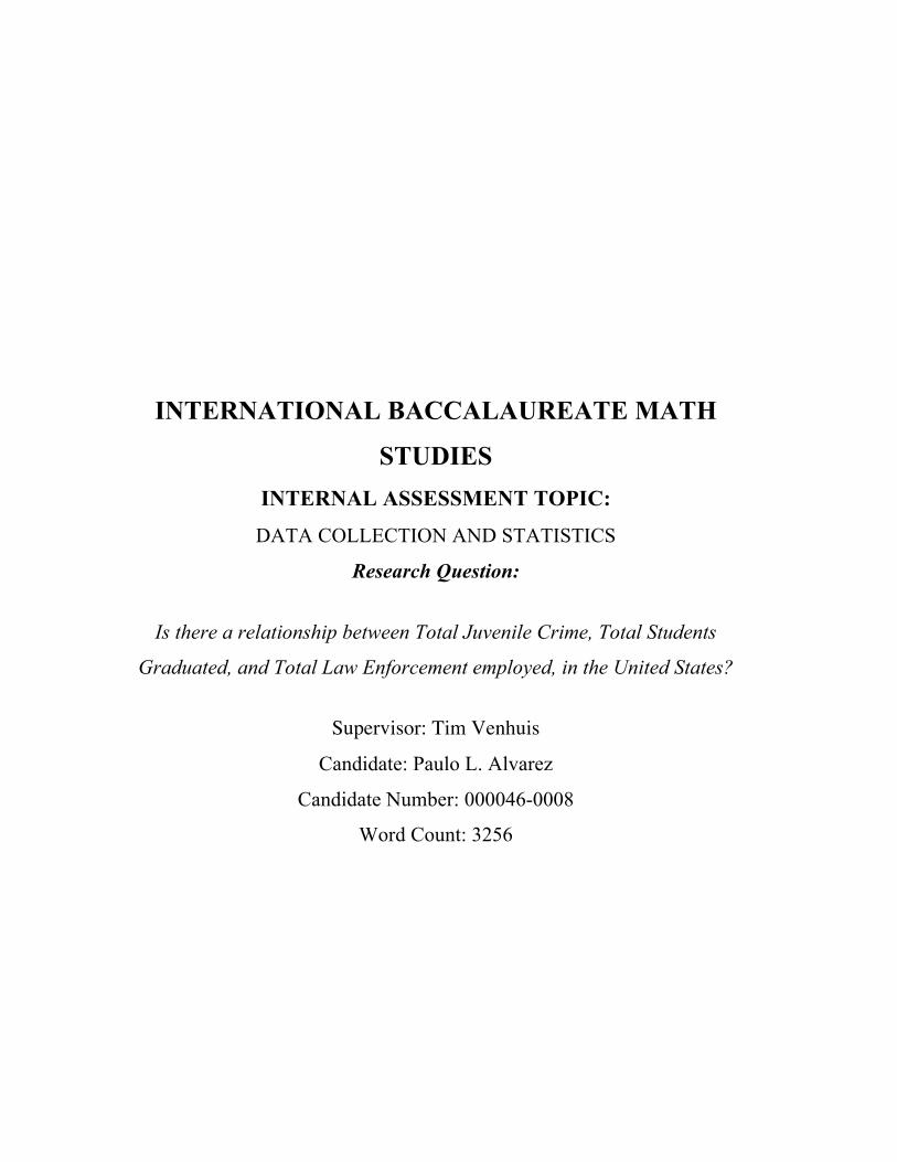
Median   83   309,915   247,105  

Column Graphs 1, 2, and 3:

Column Graphs: An advantage to using the column graph for visually organizing my

variables is that it highlights states that are either particularly strong or weak in a given

variable. These graphs can also be used to make an initial visual judgment regarding, in an

attempt at correlation/causation. Lastly, the column graph is useful for my project, as the

scope of it takes place in one year, and deals with 50 different subjects/states.

Graph 1: Column Graph of Total Juvenile Crimes per State in 2012

Observations:

As this investigation will be looking at the effects of High School Graduates and Law

Enforcement in a state, it is natural to start off by looking at the Total Juvenile Crimes per

State. With regards to total juvenile crimes per state in 2012, Illinois, Wisconsin, South

Dakota, Nebraska, and Wyoming make up the top five states with the highest in total crimes

reported. While California, Connecticut, Kentucky, Massachusetts, and West Virginia have

the lowest. While the investigation factors in all 50 states, these 10 states happen to be the

strongest and weakest in regards to crime, thus it could be expected that their law

enforcement employed and high school graduates would either be high for low crime and for

high crime states.

  7

Graph 2: Column Graph of Total High School Graduates per State in 2012

Graph 3: Column Graph of Law Enforcement Employed per State in 2012

Observations: With the variables that will be tested with total Juvenile Crimes, law

enforcement and total high school graduates are presented visually on graphs 2 and 3 with

some disparity. For instance there are states like California, which visually, has the most high

  8

school graduates and law enforcement employed, yet in regards to crime, isn’t the lowest

state. States like Massachusetts and West Virginia are the two lowest states regarding crime,

but visually appear to be fairly low with high school graduates and law enforcement

employed. A possible explanation for this disparity, and a potential weakness with the data

collected, is that the youth population of each state varies in levels. Going back to California,

Massachusetts, and West Virginia, California’s youth population is about 2,813,521.

Compare that to West Virginia and Massachusetts and their combined youth population of

582,747 is only about 20.7% of California’s. Hence it would be expected that California

almost acts like an outlier in that it has a significantly higher youth population than most

states, thus yielding higher graduates and law enforcement employed. However, California’s

data will not be considered as an outlier since it is a US state, and therefore qualifies as being

included in this investigation. So while at a glance these column graphs cannot be used to

support correlation/causation of the variables a stronger method to do so would be the Chi-

Square test of independence.

Chi Square Test

For my further process in this investigation, I shall use two Chi-Square tests to determine if

Total Juvenile Crimes is independent from Total High School Graduates and Total Law

Enforcement Employed. My determiners for the Chi-Square tests are going to be based on

the averages of Law Enforcement Employed; 19,027 and Total High School Graduates;

357,132. With the averages I will divide the 50 states with those that are above and including

the average, and those that are below the average. A summary of the earlier computations is

shown below:

Law Enforcement Employed Total High School Graduates (Aged 15-19)

Mean 19,027 357,132

Median 12,239 247,105

Next, with regards to Total Juvenile Crime, I have divided the total into violent and non-

violent crimes. An example in calculating the total non-violent and violent crimes, I will add

the number of Violent Crime and Property Crime reported to make up violent crimes.

  9

Likewise, I will add the number of Drug abuse and weapons possession reported to make up

non-violent crimes. Table 4: Division of Violent Crimes (Bold Red) and Non-Violent Crimes per US State in 2012

State   Violent  Crime     Property  Crime    

Drug  Abuse   Weapon  Possession  

Alabama   57   698   286   11  Alaska   246   1485   622   50  Arizona   152   1109   653   34  Arkansas   143   1001   328   44  California   225   669   253   123  Colorado   111   1108   611   65  Connecticut   162   599   211   45  Delaware   389   1245   546   73  Florida   263   1264   480   56  Georgia   169   927   302   61  Hawaii   248   826   880   67  Idaho   87   1198   549   70  Illinois   751   1395   1337   291  Indiana   160   981   387   45  Iowa   183   1347   403   49  Kansas   112   809   369   23  Kentucky   91   562   166   20  Louisiana   445   1385   477   90  Maine   54   1133   412   26  Maryland   295   1100   617   102  Massachusetts   177   305   84   28  Michigan     135   658   274   53  Minnesota   114   1267   525   47  Mississippi   63   1004   377   64  Missouri   187   1258   468   61  Montana   113   1535   406   15  Nebraska   115   1711   719   57  Nevada   243   941   405   40  New  Hampshire   54   650   543   0  New  Jersey   199   523   526   80  New  Mexico   202   1278   644   78  New  York   218   1024   485   56  North  Carolina   162   969   319   138  North  Dakota   89   1343   501   37  Ohio   100   703   252   43  Oklahoma   130   958   354   49  Oregon   133   1215   699   45  Pennsylvania   303   770   387   90  Rhode  Island   128   735   407   130  South  Carolina   146   911   516   87  South  Dakota   87   1495   1043   60  Tennessee   281   949   431   85  Texas   121   785   471   29  Utah   76   1328   492   85  Vermont   70   391   239   17  Virginia   74   620   337   41  Washington   163   1039   399   60  West  Virginia   57   323   138   10  Wisconsin   234   1793   648   143  Wyoming   51   1264   1122   66  

  10

For the first Chi-Square test that will compare the corresponding means between High

School Graduates and Juvenile Crimes, the null hypothesis and alternate hypotheses will be

presented:

High School Graduates and Juvenile Crimes

𝑯𝟎: High School Graduates and Juvenile Crimes are independent

𝑯𝟏 : High School Graduates and Juvenile Crimes are not independent  

Degrees of Freedom:

Using the Degrees of Freedom (df) Formula:

𝒅𝒇 = 𝑟 − 1 𝑐 − 1 , 𝑤ℎ𝑒𝑟𝑒  𝒅𝒇  𝑟𝑒𝑝𝑟𝑒𝑠𝑒𝑛𝑡𝑠  𝐷𝑒𝑔𝑟𝑒𝑒𝑠  𝑜𝑓  𝐹𝑟𝑒𝑒𝑑𝑜𝑚,  

𝒓  𝑟𝑒𝑝𝑟𝑒𝑠𝑒𝑛𝑡𝑠  𝑡ℎ𝑒  𝑛𝑢𝑚𝑏𝑒𝑟  𝑜𝑓  𝑟𝑜𝑤𝑠,      

𝑎𝑛𝑑  𝒄  𝑟𝑒𝑝𝑟𝑒𝑠𝑒𝑛𝑡𝑠  𝑡ℎ𝑒  𝑛𝑢𝑚𝑏𝑒𝑟  𝑜𝑓  𝑐𝑜𝑙𝑢𝑚𝑛𝑠  

𝑖𝑛  𝑡ℎ𝑒  𝐶𝑜𝑛𝑡𝑖𝑛𝑔𝑒𝑛𝑐𝑦  𝑇𝑎𝑏𝑙𝑒

𝒅𝒇                   = 2− 1 2− 1

∴ 𝒅𝒇   = 𝟏

According to the Degrees of Freedom table, below:

The data, therefore, shall be tested at a 5% significance level of 3.84.

  11

Chi Square Table 1: Average of High School Graduates in 2012 with Violent and Non

Violent Crimes Contingency Table

Crime Category

Total High School

Graduates (Aged 15-19)

Violent

Non-Violent

Total

≥ 357,132

17,325

8,073

25,398

< 357,132

41,829

19,166

60,995

Total 59,154

27,239

86,393

Expected Value Table for Average of High School Graduates in 2012 with Violent and

Non Violent crimes

Crime Category

Total High

School

Graduates

(Aged 15-19

Violent

Non-Violent

Total

≥ 357,132

59,154  ×  25,39886,393 = 17,390

27,239  ×  25,39886,393 = 8,008

25,398

< 357,132

59,154  ×  60,99586,393 = 41,764

27,329  ×  60,99586,393 = 19,231

60,995

Total

59,154

27,239

86,393

  12

𝒳!"#!!

𝑓!

𝑓! 𝑓! − 𝑓! (  𝑓! − 𝑓!)! (  𝑓! − 𝑓!)!

𝑓!

17,325

17,390

- 65

4,225

0.242

41,829

41,764

65

4,225

0.101

8,073

8,008

65

4,225

0.527

19,166

19,231

-65

4,225

0.219

Total

1.09

∴  𝒳!"#!! = 1.09

Since the 𝒳!"#!! value of 1.09 is less than the critical value of 3.84, we can reject 𝐻! and

accept 𝐻!. Therefore High School Graduates and Juvenile Crimes are independent of each

other. Because the contingency table is a 2x2 table with a df of 1, the Yates Correction for

Continuity Test must be used. The Yates test was developed by English Statistician Frank

Yates, and is meant to account for the upwards bias in a 2x2 contingency table.

Yates Correction For Continuity Test

Using the Yates Formula:

𝒳!"#$%! =

𝑓!!  𝑓! − 0.5 !

𝑓!

!

  13

Therefore in tabular form, the following values were derived:

(  𝑓! − 𝑓!)!

𝑓!  

(  𝑓! − 𝑓! − 0.5 !

𝑓!

0.242

0.239

0.101

0.996

0.527

0.519

0.219

0.216

1.09

1.07

∴ Since 1.07 < 3.84, we can now accept the 𝐻! and reject 𝐻!  to conclude that High School

Graduates and Juvenile Crimes are independent.

Now that we have tested the total high school graduates with juvenile crimes, a second test

will be performed with the second variable with juvenile crimes, the total number of law

enforcement employed.

Law Enforcement Employed and Juvenile Crimes

𝐻!: Law Enforcement Employed and Juvenile Crimes are independent

𝐻! : Law Enforcement Employed and Juvenile Crimes are not independent  

  14

Chi Square Table 2: Contingency Table of Average Law Enforcement Employed in

2012 with Violent and Non Violent crimes

Crime Category

Law Enforcement

Employed

Violent

Non-Violent

Total

≥ 19,027

19,732

8,895

28,627

< 19,027 38,447

17,806

56,253

Total

58,179

26,701

84,880

Expected Value Table for Law Enforcement Employed in 2012 with Violent and Non

Violent crimes

Crime Category

Law

Enforcement

Employed

Violent

Non-Violent

Total

≥ 19,027

58,179  ×  28,62784,880 = 19,622

26,701×  28,62784880 = 9,005

28,627

  15

< 19,027

58,179  ×  56,25384,880 = 38,557

27,329  ×  60,99584,880 = 17,696

56,253

Total

58,179

26,701

84,880

𝒳!"#!!

𝑓!

𝑓! 𝑓! − 𝑓! (  𝑓! − 𝑓!)! (  𝑓! − 𝑓!)!

𝑓!

19,732

19,622

110

12,100

0.616

38,447

38,557

-110

12,100

0.313

8,895

9,005

-110

12,100

1.34

17,806

17,696

110

12,100

0.683

Total

2.95

∴  𝒳!"#!! = 2.95

Yates Correction For Continuity Test Since the 𝒳!"#!

! value of 2.95 is less than the critical value of 3.84, we can reject 𝐻! and

accept 𝐻!. Therefore Law Enforcement and Juvenile Crimes are independent of each other.

Similar to the first Chi-Square Table, this contigency table is a 2x2 table and has a df of 1.

Hence it must go through the Yates Continuity Test before comparing to the df of 3.84. I

used use my Ti-84 graphing calculator and produced the following values:

  16

(  𝑓! − 𝑓!)!

𝑓!  

(  𝑓! − 𝑓! − 0.5)!

𝑓!

0.2429557217

0.6110615636

0.1011636816

0.3109746609

.5275974026

1.331510272

.2196973636

0.677568377

2.957944161

2.931114874

∴ 2.931114874 < 3.84 we can now accept the 𝐻! and say that High School Graduates and

Juvenile Crimes are independent.

Conclusion

In exploring the relationship between Total Juvenile Crimes with total high school graduates

and total law enforcement employed, I have used two Chi-Square tests then subsequently

used the Yates Correction for Continuity test, as my contingency tables are 2x2 and yield a

degrees of freedom of 1. I’d then compare the values yielded by the Yates test, and found

that for total high school graduates, the sum of (  !!!!!!!.!)!

!! = 1.074687763 which is less than

the significance level of 3.84 thus the relationship between Total High School Graduates and

Total Juvenile Crimes, is independent. For Total Law Enforcement Employed, the sum of (  !!!!!!!.!)!

!! = 2.931114874 is less than 3.84, hence the relationship between Total Law

Enforcement and Total High School Graduates is independent. Thus, it can be concluded that

Total Juvenile Crimes has no relationship with both Total Law Enforcement Employed and

the Total High School Graduates in a given US State. In this investigation I had faced some

issue with the extent of the data collected and used. For instance the data used came from

  17

2012, nearly four years have passed since then and the numbers in regards to the variables

used may have changed substantially. The reason I had used 2012 as the basis of my

investigation, is because no other year beyond 2012 has a complete set of data that I needed,

specifically the number of total High School Graduates in a given state. I also acknowledge

that the reliability of the data source could come under question, as all of the data used in this

investigation are from government sources, and the extent to which the data is true or inflated

due to different criteria for all 50 states may be troublesome to the overall data. Lastly,

regarding the nature of this issue, the scope used may not be adequate as the investigation

only focused on Juvenile crimes. When it may be possible that a student may commit a

crime later in their lives.

  18

Works Cited Page

"State Population by Age and Gender: Census 2000, 2010 and Change | Fastest Growing States." State Population by Age and Gender: Census 2000, 2010 and Change | Fastest Growing States. Proximity, 2012. Web. 10 Jan. 2016.

United States of America. Department of Justice. Office of Juvenile Justice and Delinquency Prevention. Office of Juvenile Justice and Delinquency Prevention Juvenile Arrests 2012. By Charles Puzzanchera. US Department of Justice, Dec. 2014. Web.

United States of America. Federal Bureau of Investigation. Criminal Justice Information Service Division. Full-time Law Enforcement Employees. By CJIS. N.p.: n.p., 2012. FBI Crime in the US. Web.

United States of America. Federal Bureau of Investigation. Criminal Justice Information Service Division. Violent Crime. By CJIS. N.p.: n.p., 2013.FBI Crime in the US 2013. Web.