alternative approaches for resale housing price indexes · deleted sparse observation on the tails...

Alternative Approaches for Resale Housing Price Indexes

by Erwin Diewert University of British Columbia and

University of New South Wales

Ning Huang Statistics Canada

and Kate Burnett-Isaacs

Statistics Canada

15th Meeting of the Ottawa Group Eltville am Rhein, May 10, 2017

Germany

1

Introduction

• In order to fill out the cells in a nation’s balance sheets, it is necessary to decompose property value into land and structure components.

• Information on the amount of land (and its price) is necessary in order to determine the productivity performance of the country.

• The problem is that information on the value of the land component of property value is almost completely lacking.

• Thus in this paper, we will attempt to partially fill this statistical gap by indicating how residential property values could be decomposed into land and structure components.

• We also look at alternative models of depreciation and compare alternative hedonic regression models

2

Data

• The data for this study were obtained from the Multiple Listing Service for the city of Richmond, British Columbia, Canada for 36 quarters: Q1 in 2008 to Q4 in 2016.

• We started out with 13,199 sales of detached houses but we deleted sparse observation on the tails of the distribution of selling prices and on the distribution of the characteristics used to describe the properties.

• We ended up with 11,045 observations. • The main price determining characteristics of the properties

are the area of the land plot L, the floor space area of the structure S, the age A of the house and its location (postal code area).

• We had information on the above characteristics plus a few additional characteristics.

3

Data (continued)

The ranges of the variables that we used are as follows:

• The land plot area L is between 3000 and 12000 square feet; • Floor space area S (also called living area or structure area)

is between 1000 and 4800 square feet; • The age A of the structure is less than or equal to 60 years; • The structure has 1 to 6 bathrooms (NBA); • The structure has 3 to 7 bedrooms (NBE); • The structure has 1 to 3 kitchens; • The structure has less than 4 covered parking spots; • For the sales prices, we deleted the bottom 1% and

approximately the top 3% of selling prices by year.

4

Data (continued)

• We did not use the kitchen or parking characteristics in our regressions; these variables were used to eliminate properties with an unusual number of kitchens or parking spots.

• In addition to the above variables, we had information on which one of 6 postal code regions for Richmond was assigned to each property.

• Finally, we used a quarterly residential construction cost index for the Metropolitan Area of Vancouver which we denote as pSt for quarter t = 1,...,36.

• This index (in dollars per square foot of floor space area) is derived from Statistics Canada residential house construction cost models for Metro Vancouver.

• In the following Table, V denotes the value of the property; i.e., the selling price.

5

Data (concluded)

• Table 1: Descriptive Statistics for the Variables

6

Name No. of Obs. Mean Std. Dev Minimum Maximum Unit of Measurement V 11045 $1134.1 473.61 $450 $3435 1000 dollars A 11045 26.093 16.746 0 60 No. of Years L 11045 6.5101 1.8720 3.003 12.000 1000 ft2

S 11045 2.6196 0.7507 1.000 4.793 1000 ft2 NBA 11045 4.3928 0.9789 3 7 Number NBE 11045 3.5283 1.2768 1 6 Number

3. The Builder’s Model

• The builder’s model for valuing a detached dwelling unit postulates that the value of the property is the sum of two components: the value of the land which the structure sits on plus the value of the structure.

• The simplest model for a new structure is the following one: (1) Vtn = αtLtn + βtStn + εtn ; t = 1,...,36; n = 1,...,N(t). • Older structures will be worth less than newer structures due

to the depreciation of the structure. • Assuming that we have information on the age of the

structure n at time t, say A(t,n), a more realistic hedonic regression model than that defined by (1) above is the following basic builder’s model (with geometric depreciation):

(2) Vtn = αt Ltn + βt(1 − δ)A(t,n)Stn + εtn ; t = 1,...,36; n = 1,...,N(t)

where δ is the annual structure depreciation rate. 7

The Builder’s Model with Geometric Depreciation

• Note that the above model is a supply side model as opposed to a demand side model.

• Basically, we are assuming competitive suppliers of residential properties so that we are in Rosen’s (1974; 44) Case (a), where the hedonic surface identifies the structure of supply.

• This assumption is justified for the case of newly built houses but it is less well justified for sales of properties with older structures where a demand side model may be more relevant.

• Experience has shown that it is usually not possible to estimate sensible land and structure prices in a hedonic regression like that defined by (2) due to the multicollinearity between lot size and structure size.

8

Builder’s Model 1

• Thus in order to deal with the multicollinearity problem, we replace the parameter βt in (2) by pSt, the period t Statistics Canada construction cost price for houses in the Greater Vancouver area and we obtain the following Model 1:

(3) Vtn = αt Ltn + pSt(1 − δ)A(t,n)Stn + εtn .

• This model has 36 quarterly land price parameters (the αt) and one (net) geometric depreciation rate δ.

• The R2 (between the observed values and the predicted values) was 0.7233 which is not too bad for such a simple model.

• The estimated depreciation rate was 2.85% per year. • Land prices grew from α1 = $74.16 per ft2 in the first quarter

of 2008 to α36 = $214.00 per ft2 in the last quarter of 2016, a 2.89 fold increase over the sample period.

9

Builder’s Model 2

• In order to take into account possible neighbourhood effects on the price of land, we introduced postal code dummy variables, DPC,tn,j, into the hedonic regression (3).

• These 5 dummy variables are defined as follows: for t = 1,...,36; n = 1,...,N(t); j = 1,...,5:

(4) DPC,tn,j ≡ 1 if observation n in period t is in Postal Code j of Richmond; ≡ 0 if observation n in period t is not in Postal Code j of Richmond. • We now modify the model defined by (3) to allow the level of

land prices to differ across the 6 postal codes in Richmond. The new nonlinear regression Model 2 is the following one:

(5) Vtn = αt(∑j=16 ωjDPC,tn,j)Ltn + pSt(1 − δ)A(t,n)Stn + εtn.

10

Builder’s Model 2 (continued)

• Comparing the models defined by equations (3) and (5), it can be seen that we have added an additional 6 neighbourhood relative land value parameters, ω1,...,ω6, to the model defined by (3).

• However, looking at (5), it can be seen that the 36 land time parameters (the αt) and the 6 location parameters (the ωj) cannot all be identified.

• Thus we need to impose at least one identifying normalization on these parameters.

• We chose the following normalization (the 4th postal code region had the most observations)

(6) ω4 ≡ 1. • Note that if we initially set all of the ωj equal to unity, Model

2 collapses down to Model 1; i.e., the models are nested.

11

Builder’s Model 2: Results

• The final log likelihood for Model 2 was an improvement of 892.96 over the final LL for Model 1 (for adding 5 new neighbourhood parameters) which of course, is a highly significant increase.

• The R2 increased to 0.7662 from the previous model R2 of 0.7233.

• The new estimated depreciation rate turned out to be 0.0274 or 2.74% per year (previous model was 2.85% per year).

• The price of land increased 2.90 fold over the sample period (the previous model generated a 2.89 fold increase).

• There are significant neighbourhood effects! • Up to this point, we have assumed that land plots in the same

neighbourhood sell at a constant price per square foot of lot area. In our next model, we see if there is some nonlinearity in the price of land as lot size increases. 12

Builder’s Model 3

• In order to capture lot size nonlinearity, we divided up our 11,045 observations into 7 groups of observations based on their lot size.

• For each observation n in period t, we define the 7 land dummy variables, DL,tn,k, for k = 1,...,7 as follows:

(7) DL,tn,k ≡ 1 if observation tn has land area that belongs to group k; ≡ 0 if observation tn has land area that does not belong to group k. • These dummy variables are used in the definition of the following

piecewise linear function of Ltn, fL(Ltn), defined as follows: (9) fL(Ltn) ≡ DL,tn,1λ1Ltn + DL,tn,2[λ1L1+λ2(Ltn−L1)] + DL,tn,3[λ1L1+λ2(L2−L1)+λ3(Ltn−L2)] + ... + DL,tn,7[λ1L1+λ2(L2−L1)+ ... + λ6(L6−L5)+λ7(Ltn−L6)] • where the λk are unknown parameters and L1 ≡ 4, L2 ≡ 5, L3 ≡ 6,

L4 ≡ 7, L5 ≡ 8 and L6 ≡ 9. (We are splining the land area). 13


• The function fL(Ltn) defines a relative valuation function for the land area of a house as a function of the plot area.

• The new nonlinear regression Model 3 is the following one: (10) Vtn = αt(∑j=1

6 ωjDPC,tn,j)fL(Ltn) + pSt(1 − δ)A(t,n)Stn + εtn ; t = 1,...,36; n = 1,...,N(t). • Comparing Models 2 and 3, it can be seen that we have

added an additional 7 land plot size parameters, λ1,...,λ7, to the model defined by (5).

• We impose the following identification normalizations on the parameters for Model 3:

(11) ω4 ≡ 1; λ5 ≡ 1. • If we set all of the λk equal to unity, Model 3 collapses down

to Model 2. 14


• The final log likelihood for Model 3 was an improvement of 1761.68 over the final LL for Model 2 (for adding 6 new lot size parameters) which is a highly significant increase.


• The new estimated depreciation rate turned out to be 0.0405 or 4.05% per year.

• The price of land increased 2.69 fold over the sample period. • The sequence of marginal land prices generated by this

model are as follows: λ1 = 1.1350, λ2 = 0.6915, λ3 = 0.1198, λ4 = 0.2963, λ5 = 1.0000 (this value was imposed), λ6 = 0.3871 and λ7 = 0.0086. Thus the marginal land prices as functions of lot size are not monotonic but for very large land plots, the marginal price of an extra square foot of land is very low.

15

Builder’s Model 4

• We now allow the marginal price of adding an extra amount of structure to vary as the size of the structure increases.

• In order to capture this nonlinearity, we divided up our 11,045 observations into 5 groups of observations based on their structure size.

• The Group 1 properties had structures with floor space area less than 2,000 ft2, …

• The Group 5 properties had structure areas greater than or equal to 3,500 ft2.

• 5 structure dummy variables, DS,tn,m, were defined as follows: (12) DS,tn,m ≡ 1 if observation tn has structure area that belongs to structure group m; ≡ 0 if observation tn has structure area that does not belong to group m.

16


• These dummy variables are used in the definition of the following piecewise linear function of the structure area variable S, gS(Stn), defined as follows:

(13) gS(Stn) ≡ DS,tn,1µ1Stn + DS,tn,2[µ1S1+µ2(Stn−S1)] + DS,tn,3[µ1S1+µ2(S2−S1)+µ 3(Stn−S2)] + DS,tn,4[µ1S1+µ2(S2−S1)+µ3(S3−S2) + µ4(Stn−S3)] + DS,tn,5[µ1S1+µ2(S2−S1)+µ3(S3−S2)+µ 4(S4−S3)+µ 5(Stn−S4)]. • where the µm are unknown parameters and S1 ≡ 2, S2 ≡ 2.5,

S3 ≡ 3 and S4 ≡ 3.5. • The function gS(Stn) defines a relative valuation function for

the structure area of a house as a function of the structure area.

17


• The new nonlinear regression model is the following Model 4:

(14) Vtn = αt(∑j=16 ωjDPC,tn,j)fL(Ltn) + pSt(1 − δ)A(t,n) gS(Stn) + εtn ;

t = 1,...,36; n = 1,...,N(t). • Comparing the models defined by equations (10) and (14), it

can be seen that we have added an additional 5 structure floor space parameters, µ1,...,µ5, to the model defined by (10).

• Again, we add the normalizations (11) in order to identify all of the parameters in the model.

• There are a total of 53 unknown parameters in Model 4. • Note that if we set all of the µm equal to unity, Model 4

collapses down to Model 3.

18


• The final log likelihood for Model 4 was an improvement of 934.91 over the final LL for Model 3 (for adding 5 new structure size parameters).

• The R2 increased to 0.8520 from the previous model R2 of 0.8283. • The new depreciation rate turned is 0.0298 or 2.98% per year. • The price of land increased 3.34 fold over the sample period. • The sequence of marginal land prices generated by this model are

as follows: λ1 = 1.3042, λ2 = 0.7729, λ3 = 0.2613, λ4 = 0.3536, λ5 = 1.0000 (this value was imposed), λ6 = 0.6410 and λ7 = 0.1268.

• The marginal structure floor space prices estimated by Model 4 were as follows: µ1 = 1.4318, µ2 = 1.1697, µ3 = 1.5871, µ4 = 2.4859, µ5 = 0.6222.

• Thus there is a considerable amount of variability in both the marginal land and structure price parameters.

19

Builder’s Model 5

• In Model 5, we allowed the geometric depreciation rates to differ after each 10 year interval.

• For each observation n in period t, we define the 6 age dummy variables, DA,tn,i, for i = 1,...,6 as follows:

(15) DA,tn,i ≡ 1 if observation tn has structure age that belongs to age group i; ≡ 0 if observation tn has structure age that does not belong to age group i. • Define the following function of the age variable, gA(Atn): (16) gA(Atn) ≡ DA,tn,1(1−δ1)A(t,n) + DA,tn,2(1−δ1)10(1−δ2)A(t,n)−10 + DA,tn,3(1−δ1)10(1−δ2)10(1−δ3)A(t,n)−20

+ DA,tn,4(1−δ1)10(1−δ2)10(1−δ3)10(1−δ4)A(t,n)−30 + DA,tn,5(1−δ1)10...(1−δ4)10(1−δ5)A(t,n)−40 + DA,tn,6(1−δ1)10...(1−δ5)10(1−δ6)A(t,n)−50.

20


• The new Model 5 nonlinear regression model is the following one:

(17) Vtn = αt(∑j=16 ωjDPC,tn,j)fL(Ltn) + pStgS(Stn)gA(Atn) + εtn .

• Comparing the models defined by equations (14) and (17), it can be seen that we now have 6 depreciation rates, δ1,...,δ6, in place of the single depreciation rate δ which appeared in Model 4.

• Again, we add the normalizations (11) in order to identify all of the parameters in the model.

• There are a total of 58 unknown parameters in Model 5. • Note that if we initially set all of the δi equal to the δ which

appeared in Model 4, then Model 5 collapses down to Model 4.

21


• The final log likelihood for Model 5 was a modest improvement of 24.36 over the final LL for Model 4 (for adding 5 new depreciation rate parameters).


• Using this model, the price of land increased 3.34 fold over the sample period, the same increase as occurred in Model 4.

• The new decade by decade estimated depreciation rates turned out to be as follows: δ1 = 0.0351, δ2 = 0.0229, δ3 = 0.0267, δ4 = 0.0462, δ5 = 0.0220 and δ6 = −0.0239.

• Thus properties with structures which are over 50 years old tend to have a negative depreciation rate; i.e., the value of the structure tends to increase by 2.39% per year.

• The marginal land and structure prices did not change much from the estimates from Model 4.

22

Builder’s Model 6

• For our final two models, we introduce bathroom and bedroom variables into the hedonic regressions.

• The number of bathrooms (NBAtn) in our sample ranged from 1 to 6 bathrooms.

• We assume that the number of bathrooms in the structure affects the quality of the structure. Thus define the following 6 dummy variables,

(18) DBa,tn,i ≡ 1 if observation n in period t is a house with i bathrooms; ≡ 0 if observation n in period t does not have i bathrooms. • We use the bathroom dummy variables defined above in

order to define the following bathroom quality adjustment function:

(19) gBa(NBAtn) ≡ (Σi=16 ηiDBa,tn,i)NBAtn.

23



(20) Vtn = αt(∑j=16 ωjDPC,tn,j)fL(Ltn)

+ pStgS(Stn)gA(Atn)gBa(NBAtn) + εtn . • Comparing the models defined by equations (17) and (20), it

can be seen that we now have added 6 new bathroom parameters, η1,...,η6, to Model 5.

• Not all of these new parameters can be identified so we impose the identifying normalizations (21):

(21) ω4 ≡ 1; λ5 ≡ 1; η3 ≡ 1. • There are a total of 63 unknown parameters in Model 6. • Note that if we initially set all of the ηi equal to 1, then Model

6 collapses down to Model 5. 24


• The final log likelihood for Model 6 was an improvement of 38.08 over the final LL for Model 5 (for adding 5 new bathroom parameters).

• The R2 increased to 0.8536 from the previous model R2 of 0.8526. • The price of land again increased 3.34 fold over the sample period,

the same increase as occurred in Models 4 and 5. • The new bedroom parameters turned out to be as follows: η1 =

1.1021, η2 = 0.9368, η3 = 1.000 (imposed), η4 = 0.9526, η5 = 0.8946 and η6 = 0.9631. These estimates are reasonable.

• The new decade by decade estimated depreciation rates turned out to be: δ1 = 0.0339, δ2 = 0.0242, δ3 = 0.0304, δ4 = 0.0445, δ5 = 0.0202 and δ6 = −0.0237. These rates are similar to the depreciation rates generated by the previous model.

• The marginal land and structure prices did not change much from the previous estimates from Models 4 and 5. 25

Builder’s Model 7

• Finally, we introduce the number of bedrooms into the hedonic regressions.

• The number of bedrooms in our sample ranged from 3 to 7 bedrooms.

• Thus define the following 5 dummy variables, DBe,tn,i, for t = 1,...,36; n = 1,...,N(t); i = 3,4,...,7:

(22) DBe,tn,i ≡ 1 if observation n in period t is a house with i bedrooms; ≡ 0 if observation n in period t does not have i bedrooms. • We use the bedroom dummy variables defined above in

order to define the following bedroom quality adjustment function, gBe(NBEtn):

26


(23) gBe(NBEtn) ≡ (Σi=37 θiDBa,tn,i)NBEtn.


(24) Vtn = αt(∑j=16 ωjDPC,tn,j)fL(Ltn)

+ pStgS(Stn)gA(Atn)gBa(NBAtn)gBe(NBEtn) + εtn

• We have added 5 new bedroom parameters, θ3,...,θ7, to Model 6.

• We impose the following normalizations: (25) ω4 ≡ 1; λ5 ≡ 1; η3 ≡ 1; θ5 = 1. • There are a total of 67 unknown parameters in Model 7. • Note that if we set all of the θi equal to 1, then Model 7

collapses down to Model 6.

27


• The final log likelihood for Model 7 was a big improvement of 180.70 over the final LL for Model 6 (for adding 4 new bathroom parameters).

• The R2 increased to 0.8583 from the previous model R2 of 0.8536. • The price of land increased 3.50 fold which is an increase over the

3.34 fold increase that occurred in Models 4-6. • The estimated coefficients for Model 7 are listed in Table 2 of the

paper. • The new estimated depreciation rates are as follows (the

corresponding rates from Model 6 are listed in brackets): δ1 = 0.0298 (0.0339), δ2 = 0.0202 (0.0242), δ3 = 0.0301 (0.0304), δ4 = 0.0345 (0.0445), δ5 = 0.0132 (0.0202) and δ6 = −0.0180 (−0.0237).

• The standard errors on the δi are fairly large and hence the depreciation parameters are not estimated with great precision.

28

Section 4. Sales Price Indexes for the Geometric Depreciation Models

• Once the parameters for Model 4 have been determined, the predicted constant quality amount of land for property n sold during period t, Ltn

*, can be defined as follows: (26) Ltn

* ≡ (∑j=16 ωjDPC,tn,j)fL(Ltn) ; t = 1,...,36; n = 1,...,N(t).

• The corresponding quarter t constant quality land price is the estimated coefficient, αt, for t = 1,...,36.

• Similarly, the predicted constant quality amount of structure for property n sold during period t, Stn

*, can be defined as follows:

(27) Stn* ≡ (1 − δ)A(t,n) gS(Stn) ; t = 1,...,36; n = 1,...,N(t).

• The corresponding quarter t constant quality structure price is the quarter t Statistics Canada price index pSt for t = 1,...,36.

29

Sales Price Indexes (continued)

• In order to form an overall quarter t property price index, it is necessary to aggregate the individual property amounts of constant quality land and structure into quarterly aggregates, say Lt

* and St*.

• This task can be accomplished by simple addition. • The corresponding quarter t aggregate prices will be αt and

pSt respectively. • Rescale these price indexes so that they equal 1 in quarter 1.

Denote these normalized price indexes by PLt and PSt for quarter t.

• Normalizing the price indexes means that the corresponding quarter t quantity aggregates need to be normalized in the opposite direction.

30


• Thus for Model 4, we end up with the following definitions for the price and quantity of aggregate constant quality land and structures for each quarter t = 1,...,36:

(28) P4Lt ≡ αt/α1 ; (29) L4t

* ≡ α1 Σn=1N(t) (∑j=1

6 ωjDPC,tn,j)fL(Ltn) ; (30) P4St ≡ pSt/pS1 ; (31) S4t

* ≡ pS1Σn=1N(t) (1 − δ)A(t,n) gS(Stn).

• P4Lt and P4St, are listed in Table 4 below. • We used the above land and structure aggregates to form

Fisher (1922) chained property price indexes. • These Model 4 aggregate property price indexes are listed as

P4t in Table 3 in the paper. • Later, we will show a Chart which plots the land price index.

31


• A similar procedure can be used in order to construct land and structure subindexes for Models 5, 6 and 7, P5Lt- P7Lt and P5St- P7St, along with the corresponding overall property price indexes, which we denote by P5t, P6t and P7t in Table 3.

• Note that definitions (28) and (30) are used to define the land and structure price indexes for each model but the counterparts to definitions (31) will differ for each model.

• For example, the counterpart definitions to (31) for Model 7 are the following definitions for t = 1,...,36:

(32) S7t* ≡ pS1Σn=1

N(t) gS(Stn)gA(Atn)gBa(NBAtn)gBe(NBEtn). • The structure price indexes generated by Models 4-7 are all

identical (and equal to the Statistics Canada index). • The overall property price indexes P4t - P7t along with a

simple mean and median price index are shown below.

32

Alternative Property Price Indexes

The mean and median indexes are more volatile; the other indexes P4t – P7t are very close to each other.

33

0.8

1.0

1.2

1.4

1.6

1.8

2.0

2.2

2.4

1 2 3 4 5 6 7 8 9 10 11 12 13 14 15 16 17 18 19 20 21 22 23 24 25 26 27 28 29 30 31 32 33 34 35 36

p4t p5t p6t p7t pMean pMedian

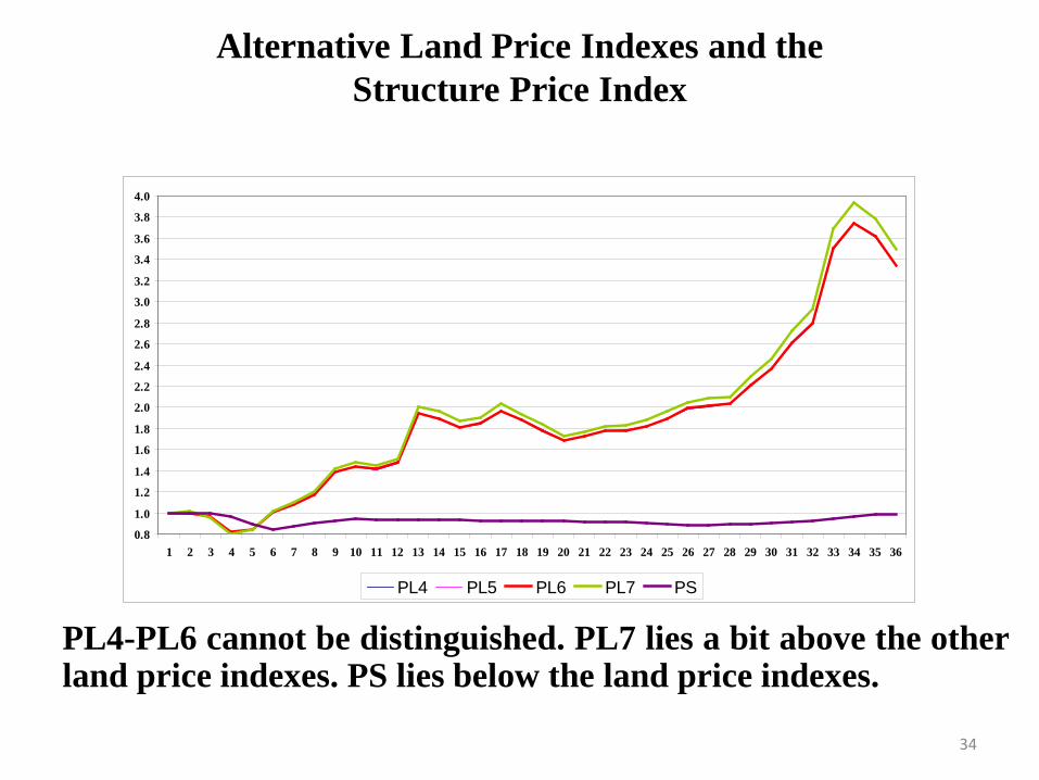
Alternative Land Price Indexes and the Structure Price Index

PL4-PL6 cannot be distinguished. PL7 lies a bit above the other land price indexes. PS lies below the land price indexes.

34

0.8

1.0

1.2

1.4

1.6

1.8

2.0

2.2

2.4

2.6

2.8

3.0

3.2

3.4

3.6

3.8

4.0

1 2 3 4 5 6 7 8 9 10 11 12 13 14 15 16 17 18 19 20 21 22 23 24 25 26 27 28 29 30 31 32 33 34 35 36

PL4 PL5 PL6 PL7 PS

Sales Price Indexes using Geometric Depreciation: Conclusion

• Our conclusion here is that it appears that Model 4, which has only a single geometric depreciation rate and does not make use of the bathroom and bedroom variables, generates land and overall property price indexes which adequately approximate our subsequent hedonic regression Models which require additional information on housing characteristics.

• This is an important result for statistical agencies in that it is typically difficult to get information on housing characteristics.

• Thus information on property location, the floor space area of the structure, the age of the structure and the lot size can be sufficient to generate price indexes that are reasonably accurate. 35

5. Approximate Price Indexes for Housing Stocks

• House price indexes are used for different purposes. • For many macroeconomic purposes, price indexes for the

sales of houses are not so important; what is more important is the construction of price indexes for the stock of houses.

• In this section, we show how our sales price indexes could be used to value residential housing stocks.

• The details in this section are omitted here. • The message in this section is as follows: once we have

estimated our hedonic regression model, then if we have characteristics information on the housing stock, we can value the stock and construct land and structure price indexes for the stock.

• For Richmond, it turns out that the stock price inflation rate is higher than the sales price inflation rate.

• The reason: sales data over represent new structures. 36

6. Sales Price Indexes for Piecewise Linear Depreciation Models

• In this section, we re-estimate Models 1-7 which were explained in Section 3.

• The geometric depreciation rates which were used in Section 3 are replaced by either straight line depreciation for Models 1-4 and by piecewise linear depreciation for Models 5-7.

• Recall that Models 1-4 were defined by equations (3), (5), (10) and (14) in Section 3.

• For the new Models 1-4, replace the term (1 − δ)A(t,n) which appears in these equations by the term (1−δAtn) so that δ is now interpreted as the straight line depreciation rate which was previously a geometric or declining balance depreciation rate.

• The parameter normalizations that were used in the geometric models are also used here.

37

Price Indexes for Piecewise Linear Depreciation Models

• Recall that Models 5-7 in Section 3 were defined by equations (17), (20) and (24).

• For the piecewise linear depreciation Models 5-7 that are estimated in this section, replace the old depreciation function gA(Atn) by the new depreciation function defined as follows (where Atn is the age of the structure on property n sold during period t and the age dummy variables DA,tn,i are defined by (15)):

(35) gA(Atn) ≡ DA,tn,1(1−δ1Atn) + DA,tn,2(1− 10δ1 − δ2(Atn−10)) + DA,tn,3(1− 10δ1 − 10δ2 − δ3(Atn−20))

+ DA,tn,4(1− 10δ1 − 10δ2 − 10δ3 − δ4(Atn−30)) + DA,tn,5(1− 10δ1 − 10δ2 − 10δ3 − 10δ4 − δ5(Atn−40)) + DA,tn,6(1− 10δ1 − 10δ2 − 10δ3 − 10δ4 − 10δ5 − δ6(Atn−50)).

38

Piecewise Linear Depreciation Models (continued)

• The remaining parts of Models 1-7 remain unchanged. • In Table 5 below, we list the R2 and improvement in the log

likelihood (∆LL) for each new model over the previous model. • For Models 1-4, we list the estimated straight line

depreciation rate δ1 for each model and for Models 5-7, we list the 6 decade by decade linear depreciation rates δ1-δ6 that were estimated by these models.

• These depreciation rates of course are somewhat different from our previously estimated geometric depreciation rates.

• However, for both the geometric depreciation Model 7 and the piecewise linear depreciation Model 7, the depreciation rate δ6 becomes an appreciation rate for structures in the 50-60 year old range.

39

Piecewise Linear Depreciation Models: Results

40

R2 ∆LL δ1 δ2 δ3 δ4 δ5 δ6 Model 1 0.7494 0.0247 Model 2 0.7914 955.60 0.0242 Model 3 0.8429 1861.43 0.0279 Model 4 0.8476 170.45 0.0210 Model 5 0.8525 181.44 0.0301 0.0140 0.0141 0.0150 0.0052 −0.0054 Model 6 0.8535 38.43 0.0292 0.0150 0.0154 0.0140 0.0047 −0.0053 Model 7 0.8583 182.55 0.0261 0.0134 0.0166 0.0123 0.0039 −0.0052

Piecewise Linear Depreciation Models: Results (continued)

• Although the estimated depreciation rates for our new Model 7 differ considerably from the geometric depreciation rates that we estimated for Model 7 in Section 3, the age functions that these two models generate are somewhat similar.

• If structure depreciation is geometric at the rate of 3% per year, the quality adjusted fraction of a structure that is A years old is g1(A) ≡ (1 − 0.03)A.

• Using the 6 decade by decade geometric depreciation rates that are listed in Table 2 and the 6 piecewise linear depreciation rates that are listed in Table 6 for Model 7, we can generate similar age functions which are denoted by g2(A) and g3(A) on Chart 1.

• It can be seen that all three age functions approximate each other closely for the first decade of age but they diverge in subsequent decades.

41

Comparing 3 Alternative Age Functions

The bottom curve is g1(A), the middle curve is g2(A) and the top curve is the age function for the piecewise linear depreciation model with 6 break points, g3(A).

42

Chart 1: Alternative Age Functions

0.00

0.20

0.40

0.60

0.80

1.00

0 3 6 9 12 15 18 21 24 27 30 33 36 39 42 45 48 51 54 57 60

g1(A) g2(A) g3(A)

Comparison of Land Prices for Models 4-7 Using Alternative Depreciation Models

• Chart 2 plots the land price indexes P4L, P6L, P7L for the geometric models and compares these indexes with the land price indexes P4LN, P6LN, P7LN for the piecewise linear models of depreciation.

• The lowest land price series P4LN, which uses a single straight line depreciation rate, generates indexes that are rather different from the other models.

• The land price indexes P4L, P6L (based on geometric depreciation) and the land price index P6LN (based on piecewise linear depreciation rates) are also too close to distinguish on Chart 2.

• The highest land price indexes are P7L and P7LN and they are too close to each other to distinguish on Chart 2.

43

Comparison of Land Prices for Models 4-7 Using Alternative Depreciation Models (continued)

44

Chart 2: Land Price Indexes Using Geometric and Piecewise Linear Depreciation Models

0.8 1.3 1.8 2.3 2.8 3.3 3.8

1 2 3 4 5 6 7 8 9 10 11 12 13 14 15 16 17 18 19 20 21 22 23 24 25 26 27 28 29 30 31 32 33 34 35 36 P4L P6L P7L P4LN P6LN P7LN

Comparison of Land Prices for Models 4-7 Using Alternative Depreciation Models: Concluded

• Our conclusion at this point is that if we use multiple depreciation rates, the price indexes that the geometric and generalized straight line depreciation generate are essentially identical.

• A more tentative conclusion is that the geometric model of depreciation with a single rate (Model 4) generates an acceptable land price index and hence also generates an overall sales property price index that approximates subsequent property price indexes based on models that require information on more characteristics.

• The depreciation rates that we have estimated in this paper do not account for all of the structure depreciation that occurs in the housing market: our data on sales of properties do not include structures which have been demolished before they reach the end of their useful life.

• Thus demolition depreciation should be taken into account.

45

7. Estimating Structure Depreciation Rates from Traditional Log Price Hedonic Regression Models • Time does not permit us to outline demand side interpretation that

can be placed on traditional time dummy variable property regressions.

• The plain vanilla traditional regression model is the following one: (41) lnVt = ρt + αlnL + βlnS + γA. • The estimates for ρt when exponentiated form a property price

index for sales of properties. • Following Shimizu, Nishimura and Watanabe (2010; 795), the

estimate for γ can be turned into a geometric depreciation rate δ for the structure:

(43) δ = 1 − eγ/β. • When we estimated a generalized version of (41) using the same

characteristics as used in our Model 7s, we found that the estimated depreciation rate generated by this log price time dummy hedonic regression was 3.003 per cent per year, which corresponds very well to our Model 4 geometric rate of 2.98 %.

46

Traditional Log Price Hedonic Regression Models (cont)

• The plain vanilla log price time dummy hedonic regression model takes the data for all quarters and estimates the α, β and γ parameters, which of course are constant across all quarters.

• Instead of running one big regression, one can take the data for 2 consecutive periods and estimate two consecutive ρt along with the α, β and γ parameters.

• Then ρt/ρt-1 can be calculated and a chained property price index can be formed.

• The advantage of this adjacent period time dummy regression model is that it allows for taste change.

• We used our Richmond data to construct property price indexes using both the one big regression approach and the chaining approach.

47

Traditional Log Price Hedonic Regression Models (cont)

• The single regression and the adjacent period overall property price indexes Pt and PCHt are plotted on Chart 3 below along with our final geometric depreciation property price index P7t and the mean and median price indexes PMean and PMedian for comparison purposes.

• From viewing Chart 3, it can be seen that the two traditional log price time dummy property price indexes, Pt and PCHt, can barely be distinguished from our final geometric depreciation property price index P7t.

• This is a very encouraging result: it means that it is possible for the traditional time dummy log price hedonic regressions to generate overall property price indexes that are consistent with the overall indexes generated by the builder’s model.

48

Comparison of Traditional Log Price Hedonic Regression Model with Our Model 7 Geometric Model

49

Chart 3: Alternative Overall Property Price Indexes for Richmond

0.8 1.0 1.2 1.4 1.6 1.8 2.0 2.2 2.4

1 2 3 4 5 6 7 8 9 10 11 12 13 14 15 16 17 18 19 20 21 22 23 24 25 26 27 28 29 30 31 32 33 34 35 36 Pt PCHt P7t PMean PMedian

Comparison of Traditional Log Price Hedonic Regression Model with Our Model 7 Geometric Model: Land and Structure Prices

50

Chart 4: Alternative Land and Structure Price Indexes

0.7

1.2

1.7

2.2

2.7

3.2

3.7

1 2 3 4 5 6 7 8 9 10 11 12 13 14 15 16 17 18 19 20 21 22 23 24 25 26 27 28 29 30 31 32 33 34 35 36 PLt PCHLt P7Lt PSt PCHSt P7St

Comparison of Traditional Log Price Hedonic Regression Model with Our Model 7 Geometric Model: Land and Structure Prices

• Chart 4 above looks at the land and structure price subindexes that can be derived from the log price time dummy hedonic regression models.

• PLt is the land price index that is implied by the one big time dummy hedonic regression;

• PCHLt is the land price index that is implied by the adjacent period time dummy hedonic regression models;

• P7Lt is the land price index generated by the geometric depreciation version of Model 7;

• PSt, PCHSt and P7St are the structure price counterparts to the above land price indexes.

• Note that while the traditional time dummy hedonic regression models generate overall price indexes that are similar to our builder’s model price indexes, this correspondence does not hold for the land and structure subindexes.

51

Conclusion

• The builder’s model can generate reasonable overall house price indexes along with reasonable land and structure subindexes using just four characteristics: the land plot area L, the structure floor space area S, the age of the structure A and the location of the property (typically the postal code).

• Introducing spline segments for the land and structure area of a property does lead to a massive improvement in the fit of the builder’s model.

• It is useful to introduce multiple depreciation rates for different ages of the structure in terms of improving the fit of the model. However, a single geometric depreciation rate does provide an adequate approximation to the more complex models for the Richmond data.

52

Conclusion (continued)

• Once we introduce multiple age dependent depreciation rates, the geometric and piecewise linear depreciation models generate virtually identical indexes. This conclusion does not hold if we have only a single depreciation rate for both types of model.

• In countries with rapidly rising residential land prices (such as Australia and Canada), the inflation rate that is generated by estimating a sales price index will tend to understate the corresponding house price inflation rate for the stock of housing.

• Simple mean and median property price indexes generated property price indexes that captured the trend in our constant quality property price indexes. However, these indexes are much more volatile than our hedonic property price indexes (as is well known).

53

Conclusion (the end!)

• The traditional log price time dummy hedonic regression approach generated overall property price indexes which were virtually identical to our builder’s model overall property price indexes when both types of model used the maximum number of characteristics.

• The traditional log price time dummy hedonic regression approach generated an implied geometric structure depreciation rate which was virtually identical to the single geometric depreciation rate generated by the builder’s model. This is a very encouraging result.

• However, our demand side utility interpretation of the traditional log price time dummy hedonic regression approach did not generate reasonable land and structure subindexes (and we explained why this result holds). The builder’s supply side model seems to generate much more reasonable results.

54

alternative approaches for resale housing price indexes · deleted sparse observation on the tails...

Documents