BPEA Conference Drafts, March 23–24, 2017

Along the watchtower: The rise and fall of U.S. low-skilled immigration

Gordon Hanson, University of California, San Diego

Chen Liu, University of California, San Diego

Craig McIntosh, University of California, San Diego

Along the Watchtower: The Rise and Fall of U.S. Low-Skilled Immigration

Gordon Hanson, UC San Diego and NBER

Chen Liu, UC San Diego

Craig McIntosh, UC San Diego

March 2017

From the rhetoric during and since the 2016 presidential election, one would think that the United States continues to experience a surge of low-skilled immigration. Although in previous decades such labor inflows certainly occurred, since the Great Recession U.S. borders have become a far less active place when it comes to the net arrival of foreign labor. The number of undocumented immigrants has declined in absolute terms, while the overall population of low-skilled foreign-born workers has remained stable. In this paper, we examine how the scale and composition of low-skilled immigration in the United States has evolved over time and how relative income growth and demographic shifts in the Western Hemisphere have contributed to the recent immigration slowdown. Because major source countries for U.S. immigration are now seeing and will continue to see weak labor-supply growth relative to the United States, the future immigration of young low-skilled workers looks set to decline further, whether or not U.S. immigration policies take a more draconian turn. We thank Janice Eberly, Adriana Kugler, and Edward Lazear for helpful comments on an earlier draft, Daniel Leff for excellent research assistance, and the Center on Global Transformation at UC San Diego for financial support.

1

Introduction Immigration is a prominent and divisive issue in public discourse about U.S. economic policy. From the rhetoric on the campaign trail over the course of the 2016 presidential election, one would think that the United States continues to see surges of undocumented immigration across its borders. During previous decades, such inflows undoubtedly occurred. The Pew Research Center estimates that between 1990 and 2007 the U.S. population of undocumented immigrants, which as of 2013 accounted for nearly two-thirds of the U.S. foreign-born adult population with 12 or fewer years of schooling, grew on net by an annual average of 510,000 individuals (Borjas, 2016; Passel and Cohn, 2016). These inflows contributed to a substantial overall increase in the U.S. supply of low-skilled foreign-born workers (Figure 1). Over the 1990 to 2007 period, the number of working-age immigrants with 12 or fewer years of schooling more than doubled, rising from 8.5 million to 17.8 million individuals. Since the Great Recession, however, U.S. borders have become a far less active place when it comes to net inflows of low-skilled labor from abroad. The undocumented population declined in absolute terms between 2007 and 2014, falling on net by an annual average of 160,000 individuals, while the overall population of low-skilled immigrants of working age remained stable. Viewed through the lens of the U.S. business cycle, the recent slowdown in low-skilled immigration hardly comes as a surprise (Villarreal, 2014). Construction is the second largest sector of employment for undocumented labor and the third largest among all low-skilled immigrants (Passel and Cohn, 2016). Because the collapse in the U.S. housing market helped precipitate the Great Recession (Mian and Sufi, 2014), it follows logically that the downturn in home building after 2006 would have triggered a drop in new arrivals of low-skilled foreign-born workers. Yet, there are good reasons to believe that the Great Recession may have merely advanced forward in time an inevitable reduction in low-skilled immigration. Today, around half of low-skilled immigrants are from Mexico and another one quarter are from elsewhere in Latin America and the Caribbean. Because these countries had marked declines in fertility after the late 1970s, they started to see slower growth in the size of cohorts coming of working age in the 2000s, thereby weakening a key demographic push factor for emigration (Hanson and McIntosh, 2010 and 2012). Just as relatively strong growth in U.S. GDP and Latin American labor supplies a generation ago helped initiate the great U.S. immigration wave of the late 20th century, the reversal of these conditions may be launching the United States into an era of far more modest low-skilled labor inflows (Hanson and McIntosh, 2009 and 2016). The current debate about U.S. immigration policy—with its discussion of walls at the border and mass deportations of undocumented residents—thus has something of an anachronistic feel to it. The dilemma facing the United States is not so much how to arrest massive increases in the supply of foreign labor, but rather how to prepare for a lower-immigration future. The pertinent issues for economists to address include how the scale and composition of low-skilled labor inflows have changed over time, whether the drop in inflows is primarily a cyclical phenomenon or represents a secular decline, and how the U.S. economy would adjust to an environment with

2

modest numbers of low-skilled foreign-born workers entering the labor force each year. These questions guide the analysis in this paper. We begin by summarizing trends in low-skilled immigration over the last several decades. As is well known, supplies of less-educated, foreign-born labor increased sharply after 1970, while their national origins shifted from Europe to Latin America. Perhaps less appreciated, the demographic structure of this population has also changed, moving from younger, recent arrivals toward an older, more-settled population. Which types of individuals select into immigration also appears to have changed, a pattern we examine in detail for the case of Mexico given its outsize importance as a source country for U.S. immigrants. In 1990, those having recently migrated from Mexico to the United States—as captured by the population censuses of the two countries—were drawn more heavily from just above versus just below the mean of potential labor-market earnings in Mexico (Chiquiar and Hanson, 2005). This mild positive selection weakened over the 1990s and the 2000s, such that by 2010 the population of recent Mexican immigrants was close to a random draw of working-age individuals from Mexico, with a slight over-representation of individuals from the middle of the skill distribution. Although immigrant selection captured in census data may be subject to measurement error associated with undercounts of undocumented immigrants (Fernandez-Huertas Moraga, 2011), selection patterns in these data are similar to those in the Mexican Family Life Survey, which appears less subject to missing information on the undocumented (Kaestner and Malamud, 2014). The largely neutral selection of immigrants from Mexico in terms of skill implies that any future shock to Mexican immigration—such as a dramatic further tightening of U.S. borders—would target middle-income earners in Mexico, while affecting low-wage earners in the United States. Recent changes in low-skilled immigration have occurred in a tumultuous environment for the U.S. labor market. Even prior to the economic turbulence that occurred after 2006, there were adverse changes in the demand for less-skilled labor associated with automation and increased import competition from low-wage countries (Autor and Dorn, 2013; Autor, Dorn, and Hanson, 2013; Pierce and Schott, 2015; Cortes, Jaimovich, and Siu, 2016). At the higher end of the labor market, demand for young, college-educated labor has also weakened (Beaudry, Green and Sand, 2016). Together, these changes combined to create a period low-wage growth after 2000 for all but the highest-earning U.S. workers (Valletta, 2016). To put recent changes in U.S. labor-market conditions in a global context, we compare the level and volatility of U.S. income to that in major sending countries for low-skilled immigrants. The gap between the 25th percentile of the income distribution in the United States and the 50th percentile of the income distribution in Mexico—which approximates the expected gains in earnings for the typical Mexican migrant—was stable during the 1990s and early 2000s but shrunk noticeably after 2007. Relative volatility in income growth has also changed. The Great Moderation heralded a period of steady U.S. GDP growth from the early 1980s to the mid 2000s (Bernanke, 2004), a calm that was brought to an end by the Great Recession. In Mexico and other migrant-sending nations of the Western Hemisphere, the pattern is roughly the opposite. The 1980s and early 1990s were periods of high macroeconomic volatility, whereas the 2000s were a

3

period of steady if not spectacular economic growth. Shrinking income gaps and reduced income volatility between the United States and major migrant-sending nations have eased pressures for net labor flows into the United States. Another factor contributing to the decline in low-skilled immigration is changes in U.S. enforcement against illegal labor inflows (Roberts, Alden, and Whitley, 2013). Between 2000 and 2010, the number of U.S. Border Patrol agents policing the U.S.-Mexico border doubled, from 8,600 officers to 17,500 officers, and has since remained at historically high levels. Concurrently, the U.S. government intensified immigration enforcement in the interior of the country, which led to an increase in deportations of non-criminal aliens—many of whom are apprehended through traffic stops or other routine law-enforcement operations—from 116,000 individuals in 2001 to an average of 226,000 individuals per year over 2007 to 2015.1 Increases in border enforcement, which deter potential migrants from choosing to enter to the United States (Gathmann, 2008; Angelucci, 2012), and in interior enforcement, which reduces the existing population of undocumented immigrants and may also deter future immigration, appear very likely to continue under the Trump Administration.2 Looking toward the future of U.S. low-skilled immigration, there are forces at work likely to weaken pressures for labor inflows that will remain in place for the next several decades. By the mid-1970s, the size of U.S. cohorts coming of working age was growing much more slowly than in Mexico and the rest of Latin America, creating steady pressure for migration to the United States. However, by the mid-2000s this demographic push factor had largely disappeared. Because U.S. neighbors to the south are today experiencing much slower labor-supply growth, the future immigration of young low-skilled labor looks set to decline rapidly, whether or not more-draconian policies to control U.S. immigration are implemented. If changes in global macroeconomic conditions and U.S. enforcement policy have combined to weaken recent growth in the U.S. supply of low-skilled foreign-born labor, what are the implications for U.S. labor markets? As a way of answering this question, we examine the net impact of immigration-induced changes in labor supply on U.S. labor-market tightness. To perform this analysis, we apply the approach in Katz and Murphy (1992) to CPS data, which involves modelling the relative hourly earnings of more- and less-skilled labor as a function of their relative supplies and a flexible time trend, meant to capture the evolution of labor demand. We estimate the model using earnings and employment data over the period 1976 to 2007 and then project relative earnings forward in time through 2015, using either actual labor supplies or labor supplies under counterfactual assumptions about low-skilled immigration. If,

1 Non-citizens (including legal immigrants) convicted of an aggravated felony, a drug crime, or multiple crimes involving moral turpitude are subject to deportation upon or before completion of their prison sentence. Deportations of criminal aliens also increased in the 2000s, from 73,000 in 2001 to an average of 156,000 per year over 2007 to 2015. See http://www.pewresearch.org/fact-tank/2016/12/16/u-s-immigrant-deportations-fall-to-lowest-level-since-2007/. 2 See, e.g., https://www.donaldjtrump.com/policies/immigration and Laura Meckler, “Trump Orders Wall at Mexican Border,” Wall Street Journal, January 25, 2017.

4

counterfactually, low-skilled foreign labor supply had grown at the same rate over 2008 to 2015 as it did over 1994 to 2007, our simple model implies that the wage gap between more and less-skilled labor would have been 6 to 9 percentage points higher in 2015. This finding, while not a general-equilibrium assessment of the wage impacts of U.S. immigration, illustrates the magnitude of the immigration slowdown in terms of U.S. wage pressures. To the extent that slowing low-skilled immigration puts downward pressure on the skill premium, we would expect firms to invest more in automation and other changes in production techniques that reduce reliance on low-skilled labor (Card and Lewis, 2007; Lewis, 2011), impacts that are likely to register most strongly in immigrant-intensive industries such as agriculture, construction, eating-and-drinking establishments, and nondurable manufacturing. Our work complements existing literature on immigration, much of which takes national changes in low-skilled foreign labor supply as given and examines its impact on the earnings of U.S. native-born workers.3 As is well known, estimates of the wage impacts of immigration vary widely across studies (e.g., Blau and Mackie, 2016). Results depend on how one defines the geographic scope of labor markets, skill groups within these labor markets, and the interchangeability of native- and foreign-born workers on the job (Borjas, 2003 and 2013; Card, 2001 and 2009; Ottaviano and Peri, 2012; Dustmann, Frattini, and Preston, 2013). To explain instability in the wage impacts of immigration, the literature has studied factors which may confound empirical analysis, including offsetting migration by native-born workers (Borjas, 2006), location choices of immigrant workers (Cadena and Kovak, 2016), firm-level changes in technology (Lewis, 2011), occupational downgrading by immigrant workers (Peri and Sparber, 2009; Dustmann, Frattini, and Preston, 2013), and measurement error in labor-market earnings (Aydemir and Borjas, 2011). Relative to existing work, we offer the inverse perspective of how and why low-skilled immigrant labor supply has changed. Given the abundance of research on how immigration affects U.S. wages, the factors that govern the magnitude of low-skilled immigration are understudied. Our work helps address this gap in knowledge.

I. Presence of Low-Skilled Immigrants in the U.S. Labor Force We begin our analysis with an overview of the characteristics of low-skilled immigrants in the United States and then examine how selection into U.S. migration among individuals from Mexico has changed over time. For the analysis in this section and the next, we focus on individuals of working age, defined to be those 18 to 64 years old. We utilize data from the U.S. Population Census, American Communities Survey, and Current Population Survey, and from the Mexico Population Census, as compiled by Ipums.org.

3 Other literature on the impacts of low-skilled immigration in the United States examines its consequences for local consumer prices (Cortes, 2008), the labor supply of high-skilled native-born women (Cortes and Tessada, 2011), local housing prices (Saiz, 2007), state GDP growth (Edwards and Ortega, 2016), cultural diversity (Ottaviano and Peri, 2005), and occupational employment and wages of native-born workers in local labor markets (Burstein, Hanson, Tian, and Vogel, 2017).

5

A. Characteristics of Low-Skilled Immigrants

A preliminary issue we must address is how to define low-skilled labor. When it comes to the analysis of immigration, the literature alternatively defines low-skilled workers as those with less than a high-school education (e.g., Borjas, 2003) or those with a high-school education or less (e.g., Card, 2001).4 The difference matters because those completing less than 12 years of schooling are an ever-smaller share of the U.S. native-born population but continue to account for a majority of adults in low- and middle-income countries. In the nations that send large numbers of low-skilled migrants to the United States—including Colombia, Cuba, the Dominican Republic, Ecuador, El Salvador, Guatemala, and Mexico—compulsory schooling is through grade 8 or 9, as opposed to being through age 16 in most U.S. states. The median worker in many sending countries thus has well less than the equivalent of a U.S. high-school education (Clemons, Montenegro, and Pritchett, 2008). Cross-national differences in compulsory education are manifest in the distribution of years of schooling among less-educated foreign- and native-born adults in the United States. In 1970, those not completing high school accounted for just over half of U.S. native-born adults with a high-school education or less, a share which declined to 29.4 percent in 1990 and to 16.6 percent in 2015 (Table 1). Among the U.S. foreign-born adult population with a high-school education or less, the share with less than 12 years of schooling has also fallen but from a much higher base, beginning at 65.2 percent in 1970 and dropping to 55.0 percent in 1990 and to 44.7 percent in 2015. To ensure our analysis is robust to the definition of skill, we utilize both education-based definitions of low-skilled labor.5 When viewed over the sweep of the last half century, the U.S. low-skilled foreign-born population has transformed not just in terms of its size but also in its demographic structure. These evolutions are evident in Tables 1 and 2, which present summary statistics on U.S. low-skilled foreign- and native-born individuals going back to 1970 using data from the U.S. Census and American Communities Survey. In 1970, when the presence of the foreign born in the U.S. population was at a historic low, low-skilled immigrants, in comparison to the native born, were relatively aged and likely to be female. This population came in its majority (52.9 percent) from Europe, was dominated by individuals who had arrived in the United States in 1960 or earlier (66.1 percent), and had a near majority (45.6 percent) with eight or fewer years of schooling. As the incipient immigration wave gained momentum, the composition of low-skilled immigrants became younger, more likely to have come from Latin America, and more educated. These changes were most dramatic between 1970 and 1990. During this period, the fraction of the

4 We define high-school education to mean completing 12 years of school, whether or not a degree is granted, a convention we adopt because the meaning of a high-school degree varies across countries. Throughout the paper, we use high-school education and 12 years of schooling interchangeably. 5 Education is, of course, an imperfect definition of skill. Language barriers and occupational licensing present obstacles to foreign-born workers in integrating themselves into the U.S. labor force, which may induce some immigrants to downgrade occupationally by taking jobs for which, based on their observable skills, they would appear overqualified (Lazear, 1999 and 2007; Dustmann, Frattini, and Preston, 2013).

6

foreign-born ages 18 to 33 rises from 28.6 to 43.2 percent, the fraction of males rises from 41.8 to 48.8 percent, and the fraction completing 12 years of education rises from 34.8 to 45.0 percent. In terms of origin countries, among immigrants with a high-school education or less, the fraction born in Mexico rises from 11.6 to 34.0 percent, the fraction born elsewhere in Latin America (and the Caribbean) rises from 13.2 to 23.7 percent, and the fraction born in Asia rises from 5.7 percent to 16.2 percent.6 The 1970 to 1990 increase in the shares of immigrants coming from Mexico and the rest of Latin America is even larger among those with less than a high-school education, rising from 15.4 to 47.5 percent and from 12.6 to 21.2 percent, respectively. By 1990, nearly 7 in 10 (68.7 percent) of the least-skilled U.S. immigrants of working age come from other nations in the Western Hemisphere. Durand, Massey, and Zenteno (2001) describe this era of U.S. immigration as one marked by a preponderance of itinerant workers who come to the United States to take seasonal jobs, especially on farms in the Southwest, and often return home during periods when labor demand was slack. During the two decades after 1970, the share of low-skilled immigrant workers employed in agriculture does rise, from 3.2 percent to 5.7 percent (as compared to a decline of 3.9 to 3.0 percent among the low-skilled native-born of working age), and the fraction with 10 or fewer years of residence in the United States grows from 34.0 to 45.8 percent.7 However, throughout the sample period, farm workers account for only a small share of low-skilled immigrant employment. During the first decades of the late 20th century immigration wave, low-skilled immigrants spread themselves across a wide range of jobs, while concentrating more heavily, when compared to their native-born counterparts, in agriculture, construction, eating and drinking establishments, nondurable manufacturing, and personal services. In subsequent decades, the low-skilled immigrant population has become more mature and more settled, at least when measured in terms of length of U.S. residence. By 2015, three quarters (75.1 percent) of low-skilled immigrants had resided in the United States for 11 or more years, while the share of the population ages 18 to 33 had dropped to 27.2 percent. Since 1990, the fraction of low-skilled immigrants from Mexico and the rest of Latin America has continued to rise, reaching 45.1 percent and 27.3 percent, respectively, in 2015. Among immigrants with less than a high-school education, these shares are 59.3 percent and 24.9 percent, respectively, meaning that today, nearly 9 in 10 (85.2 percent) of the least-skilled foreign-born workers are from Latin America and the Caribbean. Importantly, we see that Mexico’s dominance as a source country for low-skilled immigrants peaks in 2005, at 48.1 percent of those with a high-school education or less and 64.0 percent of those with less than a high-school education. The 4.7 percentage-point drop in Mexico’s share of the least-skilled-immigrant population over 2005 and 2015 is largely offset by Central America’s jump over the same period of 3.5 percentage points. As we will discuss in section III, demographic push factors help account for Mexico’s recent decline and Central America’s 6 Half of the 1970 to 1990 increase in low-skilled immigration from Asia (55.1 percent) is from Southeast Asia, with much of this inflow associated with a substantial but temporary rise in U.S. refugee admissions from the region that occurred following the end of the Vietnam War. 7 The question for length of U.S. residence reads, “When did this person come to live in the United States?” with the instruction, “If this person came to live in the United States more than once, print latest year.”

7

continuing gain as source regions. After Latin America, Asia remains the next most important source region of low-skilled immigration, in 2015 accounting for 15.8 percent of all low-skilled immigrants and 10.8 percent of those with less than 12 years of schooling. Over time, low-skilled immigrants have become more specialized in particular lines of work. The share employed in immigrant-intensive sectors in 2015 reaches 14.8 percent in construction (from 7.8 percent in 1990), 11.3 percent in eating and drinking establishments (from 8.7 percent in 1990), 7.2% in personal services (from 6.9% in 1990), and 6.9 percent in agriculture (from 5.7% in 1990). The one immigrant-intensive sector registering a decline in its share of low-skilled-immigrant employment is nondurable manufacturing, which includes apparel and textiles, two sectors whose overall employment in the United States has fallen sharply in recent decades due to technological change and competition from China and other low-wage countries. The transition of the U.S. low-skilled immigrant population from sojourners to settlers, first noted by Cornelius (1986) three decades ago, today appears to be largely complete. Part of this shift is the natural result of a dynamic process of immigration in which early arrivals initially dominate the population only to decline in importance as the existing stock grows and matures (Piore, 1980). However, the shift is also the result of the pronounced slowdown in low-skilled immigration since the mid 2000s, as seen in Figure 1. Because the immigration levels in Table 2 reflect changes in net immigration, they are uninformative about whether this slowdown is the result of reduced inflows of new immigrants, larger outflows of existing immigrants returning to their home countries, or some combination of the two. We next summarize evidence on changing inflows and outflows of immigrants over time. Figures 2a-2c give counts of immigrants by current age, age of arrival in the United States (inferred from years of U.S. residence), and census year for three source regions—Mexico, other countries in Latin America and the Caribbean, and Southeast Asia—which together account for the large majority of low-skilled immigration in the United States. To avoid concerns about tracking individuals who educate themselves out of the low-skilled category over time, we include all immigrants from these source regions, regardless of schooling. Several patterns are apparent in the data. First, for most current-age groups and in most census years, the largest cohorts are those arriving between 15 and 24 years of age. That is, for a given current-age group if we compare bars that have the same color (thus comparing different arrival-age cohorts in the same census year for the same current-age group) those in the 15-to-24 arrival-age category are the largest in nearly all cases. Second, between 2000 and 2010, there are substantial declines in the sizes of given arrival-age/birth-year cohorts. For individuals from Mexico arriving in the United States between ages 5 and 14, the number who are 15 to 24 in 2000 is much larger than the number who are 25 to 34 in 2010. We see similar declines in the number of Mexican immigrants who 25 to 34 years old in 2000 and the number who are 35 to 44 years old in 2010, both for the cohort arriving between ages 5 and 14 and the cohort arriving between ages 15 and 24. Similar patterns hold for immigrants from other countries in Latin America and from Southeast Asia. Declines in cohort size as measured in the census may result from mortality, return migration, or changes over time in the fraction of individuals in a cohort who are enumerated in the census. Given the

8

youth of the cohorts considered, mortality seems unlikely to explain this decline. Moreover, given that we expect enumeration rates to increase with residence in the United States, declines in enumeration seem an unlikely explanation, which leaves return migration as the most likely cause for the decline in measured immigrant cohort sizes between 2000 and 2010. The net impact of these changes is that the size of immigrant cohorts in 2010 is skewed heavily towards individuals who have more than ten years of residence in the United States. For immigrants from Mexico in 2010 (indicated by the darkest colored bars), those with less than 10 years of U.S. residence are the smallest cohort among all current age groups, a pattern that holds for other countries in Latin America and for Southeast Asia as well.

B. Presence of Low-Skilled Immigrants in the U.S. Labor Force

To consider how the presence of low-skilled immigrants in the U.S. labor force has changed in recent years, we focus on movements at annual frequencies using data from the Current Population Survey. Because the CPS only begins asking questions about nativity in 1994, our use of these data is for that year forward. We use two measures of the working-age population: raw data on body counts and these values expressed in terms of productivity-equivalent units following the weighting procedure in Autor, Katz & Kearney (2008).

Consistent with the post-1970 rise in low-skilled immigration seen in Figure 1, Figure 3 shows that the presence of the low-skilled foreign born in the U.S. working-age population rises steadily from 1994 to 2007 but has been stable since. The left panel of Figure 3 plots four measures of low-skilled immigration. The top value gives the share of the foreign born with a high-school education or less among all working-age individuals in the United States. This fraction rises from 6.5 percent in 1994 to 9.1 percent in 2007, before stabilizing in subsequent years, settling at 8.8 percent in 2015. Just under half of these foreign-born individuals were born in Mexico (43.1 percent in 1994, 47.3 percent in 2015). When we alternatively define low-skilled immigrants more narrowly as those with less than 12 years of schooling, we also see a growing immigrant presence in the U.S. working-age population, rising from 3.6 percent in 1994 to 4.5 percent in 2007 and showing little change thereafter. Individuals born in Mexico account for a high fraction of the less-than-high-school foreign-born population (61.1 percent in 1993, 64.4 percent in 2014). Body counts of low-skilled immigrants overstate their presence in the U.S. labor force to the extent that these individuals have low labor productivity relative to the average U.S. person of working age. To measure the population in terms of Productivity Equivalent Units (or PEUs), we apply the approach in Autor, Katz and Kearney (2008), which involves reweighting individuals by their projected relative earnings.8 Specifically, the weight attached to an individual is the ratio of the

8 When applying wage-based weights to the entire population, we assume that non-working individuals would earn the same average wage as full-time workers who share their age, gender, race, education and nativity profile. Because employment rates increase with potential earnings, this assumption may lead our productivity-adjusted shares of the low-skilled immigrant population to overstate shares one would

9

average weekly wage among full-time, full-year workers in her race, gender, education, and labor-market experience cell to the average weekly wage for white, male, high-school graduates with 8 to 12 years of potential work experience.9 Population shares expressed in terms of productivity-equivalent units appear in the right panel of Figure 3. These shares are naturally smaller than in the left panel, owing to the fact that low-skilled immigrant workers have low earnings relative to other U.S. workers. Using the productivity-adjusted measure, foreign-born individuals with 12 or fewer years of schooling reaches 6.5 percent of the U.S. working-age population in 2007, a share that declines slightly to 6.3 percent in 2015.10 Low-skilled immigrants tend to have high rates of labor-force participation and employment when compared to similarly skilled native-born workers (Borjas, 2016). Consequently, the population shares in Figure 3 may give an incomplete characterization of the presence of the low-skilled foreign-born workers in effective U.S. labor supply. Figure 4 reports the shares of low-skilled immigrants in total hours worked, both using raw hours (left panel) and productivity-adjusted hours (right panel). The share of total hours worked by immigrants with 12 or fewer years of schooling rises from 5.2 percent in 1994 to 8.4 percent in 2007, before falling modestly to 8.0 percent in 2015. When expressed in productivity-equivalent units, these shares are 3.6 percent, 5.8 percent, and 5.5 percent, respectively. Because undocumented immigrants account for a large share of the low-skilled immigrant population and because these individuals come in their large majority from Mexico and Central America, low-skilled foreign-born labor accounts for a relatively high fraction of employment in the states along the U.S. border with Mexico. Figure 5 plots the share of low-skilled immigrants in hours worked for in the five U.S. border states, again in terms of both raw hours and productivity-adjusted hours. Among these border states, the share of foreign-born workers with 12 or fewer years of education in total hours worked rises from 11.9 percent in 1994 to 16.2 percent in 2005 and then drops to 14.1 percent in 2015. Immigrant presence is also high in industries intensive in the use of less-skilled labor. As seen in Table 3, in 2015 immigrants with 12 or fewer years of schooling account for 29.3 percent of total hours worked in agriculture (up from 3.9 percent in 1970), 21.8 percent in personal services (up from 6.4 percent in 1970), 20.3 percent in

calculate based on “true” wage weights. This problem is partially ameliorated when we examine the share of low-skilled immigrants in total hours worked, as we do in Figure 4. 9 We construct these weights as follows. First, we divide workers into labor-market groups broken down by gender, two education categories (less than 12 years of education, exactly 12 years of education), and eight experience categories (0-4, 5-9, 10-14, 15-19, 20-20, 25-29, 30-34, and 35-39 years of potential-labor-market experience). Then, for each gender-education-experience group, we calculate the weight as average weekly earnings in each year (for full-time, full-year workers, defined to be those working at least 35 hours per week and 40 weeks a year) divided by average weekly earnings for white, male, high-school graduates with 8 to 12 years of labor-market experience. 10 The number of Mexican-born workers in the United States increased by more than 350,000 per year over the 20 years from 1980 to 2000. Negative net migration of 160,000 per year subsequent to 2007 therefore represents a drop of a half a million people per year relative to the prior trend, enough to constitute a sizeable change in the foreign-born population when cumulated over a decade of low migration.

10

construction (up from 3.9 percent in 1970), 16.8 percent in eating and drinking establishments (up from 8.3 percent in 1970), and 13.5 percent in non-durable manufacturing (up from 5.9 percent in 1970), as compared to just 5.0 percent of employment in all other industries. For these immigrant-intensive industries, future changes in low-skilled immigration matter immensely.

C. Who Chooses to Migrate to the United States? Is the increase in low-skill immigration in the United States the result of increasing immigration from countries that are relatively abundant in low-skilled labor or the result of low-skilled labor being relatively likely to select into international migration? One cannot answer this question by examining U.S. data alone. Differences in educational attainment across countries would make the average worker from, say, Mexico appear to be low skilled in the U.S. labor market, whereas at home she would fall into the middle of the earnings distribution. In seminal research, Borjas (1987) derives the conditions under which immigrants are negatively or positively selected in terms of skill. Conditions favoring negative selection—meaning that immigrants are drawn disproportionately from the bottom half of the skill distribution—are high returns to skill in the sending country relative to the receiving country and migration costs that are proportional to worker productivity (e.g., costs that have an iceberg form), which combine to give less-skilled workers a relatively strong incentive to migrate. Migration costs that are fixed in nature and a marginal utility of income that is not strongly decreasing favor positive selection of immigrants in terms of skill (Grogger and Hanson, 2011), in which case immigrants are drawn more heavily from the top half of the skill distribution. Whether immigrants are negatively or positively selected in terms of skill matters for how labor movements affect the distribution of income in sending and receiving countries and for the ease with which immigrants from low-income countries integrate themselves into high-income-country labor markets. If, for example, immigrants from Mexico are negatively selected in terms of skill, shocks that contribute to a positive net flow of labor from Mexico to the United States would tend to decrease Mexican wage inequality—by reducing Mexico’s relative supply of low-wage workers—and to increase U.S. wage inequality—by expanding the U.S. relative supply of low-wage workers. Further, immigrants who are negatively selected in terms of skill may face greater challenges in assimilating economically in the U.S. labor market and may be more likely to be a net drain on public resources (Borjas, 2016). To examine the composition of low-skilled immigration in the United States from the sending-country perspective, we focus on the case of Mexico, which is by far the largest source country for U.S. labor inflows, accounting for nearly half of all U.S. low-skilled immigrants and nearly two thirds of those with less than 12 years of schooling. We extend forward in time the analysis in Chiquiar and Hanson (2005), which utilizes the methodology in DiNardo, Fortin, and Lemieux

11

(1996) for constructing counterfactual wage distributions.11 To examine differences in the distribution of skills between Mexican residents (i.e., non-migrants in Mexico) and Mexican immigrants, we compare the actual wage density in Mexico for Mexican residents to the counterfactual wage density that Mexican immigrants in the United States would obtain were they paid according to Mexico’s prevailing wage structure. This comparison reveals from where in Mexico’s wage distribution migrants to the United States are drawn. Because this analysis projects U.S. immigrants onto Mexico’s wage distribution based on workers’ observable skills, it ignores the role of unobserved characteristics in migration and earnings. And because it takes Mexico’s current wage distribution as given, the analysis is silent about the equilibrium impact of immigration on U.S. or Mexican wages. Let f i(w|x) be the density of wages w in country i, conditional on observed characteristics x, h(x|i=MX) be the density of observed characteristics among workers in Mexico, and h(x|i=US) be the density of observed characteristics among Mexican immigrants in the United States. The density of wages that would prevail for Mexican immigrants in the United States if they were to be paid according to the price of skills in Mexico is given by,

∫ == dxUSixhxwfwg MXMXUS )|()|()( . (1)

This quantity corresponds to the counterfactual distribution of wages that arises from projecting the skill distribution of Mexican immigrants in the United States onto the current wage structure of Mexico. Although this distribution is unobserved, we can rewrite it as

dxMXixhxwfwg MXMXUS )|()|()( === ∫θ , (2)

where Mexico’s conditional wage distribution fMXi(w|x) and the skill distribution of its resident population h(x|i=MX) are observed and where

)|()|(

MXixhUSixh

==

=θ . (3)

Hence, we can obtain the counterfactual wage density that we desire in equation (1) simply by applying the appropriate weight θ to the existing distribution of wages in Mexico. To compute this weight, one can use Bayes’ Law to write,

)|Pr()Pr()|()(

xUSiUSiUSixhxh

===

= (4)

and

11 Also on the selection of immigrants from Mexico in terms of observable skill, see Feliciano (2001), Orrenius and Zavodny (2005), McKenzie and Rapoport (2007, 2011), and Akee (2010).

12

)|Pr()Pr()|()(

xMXiMXiMXixhxh

===

= . (5)

Combining (4) and (5), we obtain an expression for θ that is the ratio of the conditional probability that a Mexican-born worker resides in the United States, Pr(i=US|x)/Pr(i=MX|x), to the unconditional probability that a Mexican-born worker resides in the United States, Pr(i=US)/Pr(i=MX). We estimate these probabilities via a logit model, use the estimates to calculate θ , and apply the θ weights to estimate the counterfactual wage density in (2).12 We construct actual and counterfactual wage densities for males and females, separately, in three years, 1990, 2000, and 2010. Earnings are annual labor income for individuals ages 18 to 64. We estimate the logit regressions used to predict whether an individual born in Mexico resides in the United States separately for men and women as a function of education (7 categories based on years of schooling: 0-4, 5-8, 9, 10-11, 12, 13-15, 16 plus) and age (46 categories, one for each year in the range 18 to 64). The population is all working-age individuals in Mexico and Mexican immigrants in the United States who have resided in the country for 10 or fewer years. Results are similar when we expand the analysis to include immigrants with 20 or fewer years of U.S. residence, who constitute the large majority of working-age Mexican immigrants in the United States. Wage densities are plotted relative to mean log earnings for workers in Mexico of a given gender in a given year, such that actual wage densities are centered on zero. Figure 6 presents the results, where in each plot the dashed line is the actual wage density for Mexico and the solid line is the counterfactual wage density in Mexico for current Mexican immigrants. For the case of males, shown in the panels on the left of Figure 6, we see that in each year the actual and counterfactual densities are very similar to each other, suggesting that the observable skills of Mexican immigrants match closely those of individuals who have not migrated abroad. In 1990, the counterfactual wage density lies slightly to the right of the actual wage density, indicating that Mexican immigrants are mildly positively selected in terms of observable skill. This difference is more defined in Figure 7, which plots the difference between counterfactual and actual wage densities. In 1990, this difference, as seen in panel (a), has a negative mass just below zero and a positive mass just above zero, indicating that male immigrants are underrepresented among those who would earn slightly less than mean earnings in Mexico and overrepresented among those who would earn slightly more than mean earnings in Mexico. The slight rightward shift in the counterfactual relative to the actual wage density is also present in 2000 and 2010. However, the difference between actual and counterfactual densities becomes less pronounced over time, such that in panel (a) of Figure 7 the negative hump below zero and the 12 This method for constructing weights ignores differences in labor-force participation rates in the two countries. Whereas labor-force participation among male residents of Mexico and male Mexican immigrants in the United States are similar, labor-force participation is higher among immigrant Mexican women than among non-migrant Mexican women. Not accounting for these differences would tend to overstate negative selection among immigrants. See Chiquiar and Hanson (2005) for details and for methods to account for cross-national differences in labor-force participation.

13

positive hump above zero are smaller in 2000 than in 1990 and smaller still in 2010 relative to 1990. These changes are also seen in panel (b) of Figure 7, which reports the double difference in densities: counterfactual relative to actual wage densities in 2010 relative to this difference in either 1990 or 2000. The double difference using 2010 and 1990 is larger than that for 2010 and 2000, indicating a lessening of positive selection over time. By the time that we arrive in 2010, working-age Mexican immigrants who reside in the United States appear to be close to a random draw on the population of working-age individuals in Mexico. The panels on the right of Figure 6 repeat the analysis for women. Among women, we see evidence of stronger positive selection in 1990 and 2000 when compared to men. In each year, the rightward shift of the counterfactual wage density relative to the actual wage density is more pronounced than the corresponding density difference for males. As with males, the strength of positive selection diminishes over time, such that by 2010 the counterfactual and actual wage densities for women are very similar. We conclude that by 2010, the selection of immigrants from Mexico is close to neutral in terms of observable skill. As mentioned earlier, these results are silent about the pattern of immigrant selection in terms of unobservables. One concern about the results in Figures 6 and 7 is that we use census data to evaluate immigrant selection. Any undercount of the Mexico-born population in either Mexico or the United States that depends systematically on an individual’s age or education could result in biased estimates either of the wage density for Mexico or of the counterfactual wage density that we construct for Mexican immigrants in the United States. There is a long-standing belief among demographers that the U.S. Census undercounts undocumented immigrants in the United States (e.g., Warren and Passel, 1987). To address the undercount issue, some studies evaluate immigrant selection using data from Mexico exclusively (e.g., Ibarraran and Lubotsky, 2007). In noteworthy work, Fernandez-Huertas Moraga (2011) uses data from Mexico’s national employment survey (known by its Spanish acronym as the ENE), which follows households for five consecutive quarters and includes in the survey questions about whether household members have migrated to the United States in the period of time since the last survey was conducted. Distinct from Chiquiar and Hanson (2005), Fernandez-Huertas Moraga finds that Mexican immigrants are negatively selected in terms of skill, as captured by residuals from Mincerian wage regressions. The ENE, however, has measurement problems of its own. It suffers from high rates of attrition by households from the sample within the five-quarter survey window, which a recent National Academies of Science, Engineering, and Medicine study concludes makes it problematic as a data source for evaluating Mexican migration to the United States (Carriquiry and Majmundar, 2013). Fortunately, there is a data source that provides longitudinal data on households in Mexico and that tracks information on individuals who migrate to the United States. The Mexican Family Life Survey (MxFLS) has been conducted in three waves, 2002, 2006, and 2009, with a recontact rate of respondents between each wave of 90 percent. Importantly, the survey follows household members who migrate to the United States between waves. Kaestner and Malamud (2014) use data from the first two MxFLS waves to analyze the selection of immigrants according to various measures of skill. Similar to what one sees in census data, migrants to the United States in the

14

MxFLS are more likely to be young. In terms of education, both male and female migrants are more likely to have middle-levels of schooling (4 to 9 years for men, 4 to 12 years for women) than to have low levels of schooling (0 to 3 years). For men, but not for women, migrants are less likely to have very high levels of schooling (more than 12 years) than to have very low levels (0 to 3 years). The MxFLS also provides a measure of cognitive ability in the form of a Raven’s Progressive Matrices test score (Raven, Court, and Raven, 1983). Although cognitive ability is a frequently discussed source of skill in the analysis of earnings (e.g., Heckman and Vytlacil, 2001), few data sources provide evidence of how cognitive skills relate to migration decisions. Among both men and women, Kaestner and Malamud report no difference between migrants and non-migrants in terms of their Raven’s scores, suggesting that the two populations have a similar distribution of observable cognitive abilities. Following Fernandez-Huertas Moraga (2011), Kaestner and Malamud also examine migrant selection in terms of observable and unobservable characteristics using Mincerian wage regressions. Their analysis shows that workers with the highest predicted earnings or the highest residual earnings in the first MxFLS wave—meaning those among the top quintile of predicted or residual wage earners—are less likely to migrate but that there is no pattern of selection among lower-wage individuals. Despite problems with possible undercounts of undocumented migrants in census data, they provide a characterization of immigration selection that is comparable to that based on high-quality longitudinal micro data. Immigrants from Mexico to the United States are overrepresented among individuals whose skills place them in the middle of Mexico’s wage distribution and mildly under-represented among individuals who would be very low-wage or very high-wage earners in their home country. When we examine U.S. immigration from other sources countries, evidence of positive selection in terms of observable skills such as education is even more pronounced (Grogger and Hanson, 2011). In nearly all source countries for U.S. labor inflows, immigrants are relatively likely to come from among the more educated.13 Summary. The U.S. population of low-skilled immigrants has gone through an epochal half-century of growth, transforming from a small cadre of older immigrants from Europe to a large population of immigrants from Latin America and Asia who are nearing middle age and who have now lived in the United States for an extended period of time. Immigrants from Mexico, who account for one-half to three-fifths of the low-skilled foreign born depending on the definition of skill, are preponderantly individuals who would be middle-income earners in their birth country. As the United States looks forward to an era of weakened incentives for low-skilled immigration due to changing labor-demand and labor–supply conditions at home and abroad, it will be shocks to middle-wage workers in migrant-sending countries that matter disproportionately for who migrates. Attempts to dislodge the existing population of low-skilled immigrants, such as through recently proposed changes in U.S. immigration policy, would target a population that appears to be fairly well settled in the United States.

13 One exception to this pattern is Puerto Rico, which as an unincorporated territory of the United States is not subject to the same barriers to U.S. immigration as foreign nations (Borjas, 2008).

15

II. Labor Demand, Labor Supply, and Low-Skilled Immigration

In the following two sections, we examine factors affecting the net flow of low-skilled immigrants into the United States. We begin in this section by describing recent changes in conditions surrounding low-skilled immigration, including income differences between the United States and major migrant-sending countries, U.S. immigration policy, and relative labor-supply growth in the United States and major sending countries. We then analyze for the case of Mexico the contribution of labor-demand and labor-supply shocks to migration to the United States.

A. Income Differences between Countries Perhaps the simplest manner in which to evaluate the incentive for immigration is to compare income between countries. Beginning with Sjaastad (1962), economists have modelled immigration as an investment decision, in which the upfront cost of migration yields an income flow over time equal to the difference in earnings between the home and foreign economies. There may be considerable heterogeneity in the time horizon over which individuals consider migration (Dustmann, 2003). Seasonal workers may focus on income differences between countries no more than a few months in advance, other individuals may be uncertain about their desire to relocate permanently and so put weight on the income differences they expect to be sustained over the next several years, and still others may treat migration as a long-term decision and therefore evaluate the expected discounted difference in income streams over their full working lives. To examine high-frequency changes in the incentive for immigration, we abstract away from such heterogeneity and consider point-in-time income differences between the United States and migrant-sending countries, an approach taken in the large literature that uses the gravity model to analyze bilateral migration flows (e.g., Karemera, Oguledo, and Davis, 2000; Clark, Hatton, and Williamson, 2007; Bertoli and Moraga, 2013). Even in making point-in-time income comparisons, one faces many choices for how to measure income. One approach is to evaluate earnings for individuals with similar observable skills who were born in the same country and now live in different countries. Using data from U.S. and Mexico population censuses, Hanson (2006) reports that in 2000 the average hourly wage for a 28-to-32-year-old male with 9 to 11 years of education is $2.40 in Mexico and $8.70 among recent Mexican immigrants in the United States (these income values like those we report below are PPP-adjusted in terms of 2000 dollars). At a labor supply of 35 hours per week and 48 weeks per year, this would yield annual income gain of $10,600. Combining data from Mexico’s national survey of income and expenditure with data from the U.S. Census, Clemens, Montenegro, and Pritchett (2008) obtain similar results, estimating that in 2000 the annual income gain to migration for a 35-year-old Mexican male with 9 to 12 years of education is $9,200. Comparing migrants to non-migrants is problematic if there are unobserved characteristics that affect both the migration decision and an individual’s income-earning ability. An alternative approach is to use longitudinal data for the same individual, which allows comparisons of income

16

before and after migration. Rosenzweig (2007) uses data from the New Immigrant Survey to estimate the change in income for new U.S. permanent legal immigrants in 2003. He checks their current U.S. earnings against earnings in the last job they held in their country of origin. For a legal immigrant from Mexico with 9 to 12 years of education, the average gain in income is $15,900 (at 35 hours a week and 48 weeks a year). Comparing the same individual in two countries corrects for selection into migration associated with unobserved time-invariant individual characteristics but may introduce other complications. If in preparing to migrate individuals reduce their labor supply in a manner that diminishes income (or if negative shocks to income precipitate migration), this approach may overstate the income gains to migration.14 Evaluating how the incentive to migrate to the United States has changed across countries and over time is complicated by the fact that few countries produce annual household-survey data. This leaves one to use census data, which are amassed infrequently. Our approach is to construct income differences between countries by combing annual data on average income from national accounts with data on the variance in income as inferred from summary statistics on income inequality. Although statistics on income inequality, such as the Gini coefficient, are often constructed at a less than an annual frequency, they tend to change slowly from one year to the next (Solt, 2016), which permits interpolation of their values to create an annual series. Under the assumption that income is log normally distributed across households, which is approximately consistent with data for many countries (Pinkovskiy and Sala-i-Martin, 2009), one can use the Gini coefficient to calculate the variance of income across individuals and then combine this value with average income to construct income at different percentiles of the distribution (Grogger and Hanson, 2011).15 Given the neutral selection of immigrants from Mexico in terms of observable skills, the 50th percentile (equal to $8,800 in 2000) is a natural choice for the reference income of a prospective Mexican migrant. To select the reference income in the United States for a typical immigrant from Mexico, we choose the percentile of the U.S. income distribution that yields an income gain to migration in the year 2000 that is approximately equal to the average income gain for migrants in Hanson (2006), Clemens, Montenegro and Prichett (2008), and Rosenzweig (2007). The 25th percentile of the U.S. income distribution ($20,100 in 2000) serves this purpose. In panel (a) of Figure 8, we report the ratio of the 50th percentile of the Mexican income distribution to the 25th percentile of the U.S. income distribution, where we construct these values using Gini coefficients from the WIDER World Income Inequality Database and PPP-adjusted per capita GDP from the World Development Indicators.16 This ratio is stable in the 1990s and early 2000s, averaging 0.44 between 1990 and 2007. Over this period, a middle-income earner in Mexico 14 Since Rosenzweig (2007) examines legal immigrants, his figures are not directly comparable to Hanson (2006) or Clemens, Montenegro, and Prichett (2008), whose samples include all immigrants. 15 Suppose log income is normally distributed with mean μ and variance σ. Given an estimate of the Gini coefficient G, the standard deviation of log income is 𝜎𝜎 = √2Φ−1([𝐺𝐺 + 1]/2). The value of log income at the α quantile is then 2exp( z / 2)αµ σ −σ , where αz is the αth percentile of N(0,1). 16 Because Gini coefficients are not available in all years, we interpolate values for missing years. The series on Gini coefficients ends in 2012 in some countries and 2013 in others. We assume that Ginis in later years equal those in the last year for which data are available.

17

who chooses to become a low-income earner in the United States would see her real earnings increase by a factor of 2.3. After the Great Recession, the U.S.-Mexico income difference compresses, with the ratio of 50th-percentile of Mexican income to the 25th-percentile of U.S. income rising to an average of 0.53 between 2008 and 2015 and to 0.58 over the later period of 2011 to 2015. In panel (b) of Figure 8, we report the corresponding ratio of 50th percentile sending-country income to 25th percentile U.S. income for a composite of other countries in Latin America and the Caribbean. We choose the next-largest sending countries for which data on Gini coefficients are available (Colombia, Dominican Republic, Ecuador, El Salvador, Guatemala, Honduras, Jamaica), where we weight each country’s income by its relative share of working age low-skilled immigrants in the United States in 2000.17 The time path of relative income is similar to that for the Mexico-U.S. comparison, though the absolute income gap is larger. The income ratio is stable from 1990 to 2007, averaging 0.22, and then rises after the onset of the Great Recession, averaging 0.30 over 2008 to 2015. Since 2007, relatively slow U.S. income growth and rapid growth in neighboring countries has compressed the income gap between the United States and migration-sending nations, presumably weakening incentives for immigration. In forming expectations about future income differences between countries, prospective migrants are likely to consider not just the level of income but also its variance. Over short time horizons, higher perceived variance in income in the sending country relative to the receiving country may add to the incentive for migration. At a monthly frequency, changes in attempted undocumented migration from Mexico to the United States, as captured by apprehensions at the U.S.-Mexico border, are strongly sensitive to changes in the U.S.-Mexico real exchange rate, with attempted entry surging during periods following currency crises in Mexico (Hanson and Spilimbergo, 1999; Monras, 2015). When expanding data to include countries throughout the Western Hemisphere, emigration rates to the United States are larger for cohorts subject to a higher incidence of financial crises in their home country (Hanson and McIntosh, 2012). To characterize changes in U.S. income volatility relative to that in migrant-sending economies, panel (a) of Figure 9 reports the standard deviation in quarterly real GDP growth in Mexico and the United States for rolling eight-quarter windows covering the period 1990q1 to 2016q1. Throughout the time span, volatility in GDP growth is higher in Mexico (average eight-quarter standard deviation of 3.7 percent) than in the United States (average eight-quarter standard deviation of 2.0 percent). Yet, there are evident changes in relative volatility over time. After the 1995 peso crisis, volatility spikes in Mexico while remaining low in the United States. Over the ensuing ten years, volatility remains uniformly higher in Mexico, though well below the elevated

17 In 2000, the share of U.S. low-skilled working-age immigrants accounted for by these countries is 15.0 percent (4.1 percent for El Salvador, 2.8 percent for the Dominican Republic, 2.3 percent for Guatemala, 1.7 percent for Jamaica, 1.6 percent for Colombia, 1.3 percent for Honduras, and 1.1 percent for Ecuador). Gini coefficients are unavailable for Cuba and Haiti (2.5 and 1.5 percent of U.S. low-skilled immigrants in 2000, respectively), leading us to leave them out of Figures 8 and 9. Significant sending nations for U.S. low-skilled immigrants outside of the Western Hemisphere (and their shares of this population in 2000) include Vietnam (4.1 percent), the Philippines (2.2 percent), China (2.1 percent), Korea (1.5 percent), Germany (1.4 percent), Italy (1.2 percent), Canada (1.2 percent), India (1.2 percent), and Poland (1.1).

18

levels of crisis periods. With the onset of the Global Financial Crisis of 2008 to 2010, volatility jumps in both economies, declining thereafter to roughly equal levels. Reduced Mexico-U.S. differences in income volatility reflect the improved execution of monetary and fiscal policies in Mexico, which as in much of Latin America has helped lower inflation, reduce government debt, and stabilize GDP growth (Edwards, 2009). In panel (b) of Figure 9, we compare volatility in quarter-to-quarter GDP growth in the United States to the same migrant-sending countries examined with regard to relative GDP levels in Figure 8. Here again, we see that volatility in GDP growth in migrant-sending nations has decreased relative to the United States, which has presumably dampened pressures for cross-border labor flows.

B. U.S. Immigration Policy Low-skilled immigrants enter the United States through three channels: on permanent legal residence visas (green cards), on temporary work visas, and through undocumented entry. The tenor of political debate about immigration in the United States may tempt one to believe that the U.S. government has been lax when it comes to enforcing U.S. borders against undocumented immigration. During the 2000s, however, the country engaged in a massive buildup in enforcement efforts, with most newly committed resources allocated to the U.S. border with Mexico. To understand how changes in immigration policy may have affected incentives for low-skilled immigration, we review recent adjustments in U.S. policy mechanisms. Legal Immigration. The vast majority of low-skilled immigrants who obtain green cards do so through family sponsorship, for which visa eligibility derives from having a relative who is a U.S. citizen or legal resident, or as refugees or asylees (Rosenzweig, 2007). The number of U.S. green cards and the policies governing their allocation have been stable since 1990. In that year, the Immigration Act set the annual number of family-sponsored visas at 480,000, the annual number of employer-sponsored visas (which go primarily to skilled workers) at 140,000, and the annual number of diversity visas (allocated via lottery to countries that have historically low migration to the United States) at 55,000. Visas available to immediate relatives of U.S. citizens are uncapped, though applications for these visas may be subject to processing delays. The number of green cards given to refugees and asylees, while having no set cap, shows no trend over time, falling from 114,000 per year in the 1990s to 83,000 per year in the 2000s before rising to 109,000 per year over the 2010-2115 period.18 Any increase in low-skilled immigration via permanent legal visas thus cannot have occurred through expanded quotas for green cards. It must instead have occurred through increases in the number of low-skilled immigrants qualifying for, applying for, and receiving visas from the annual allocation of visas.19

18 A refugee is a foreign resident who is unable or unwilling to remain in her country of nationality because of fear of persecution based on race, religion, social group, or political opinion; an asylee is a foreign national who meets the conditions of a refugee and is already in the United States. A refugee is eligible to apply for a green card after one year of U.S. residence. At the beginning of each fiscal year, the President, in consultation with Congress, sets a worldwide ceiling on refugee admissions. 19 All data on legal immigration are from the U.S. Department of Homeland Security Yearbook of Immigration Statistics. See https://www.dhs.gov/immigration-statistics.

19

Qualifying for a green card under family sponsorship requires having an immediate relative who is a U.S. citizen—which gives one access to visas that are not subject to numeral limit—or a more distant relative who is a U.S. citizen or legal resident—which allows one to apply for the fixed annual allocation of green cards. Because the number of new applications exceeds the annual cap on green cards, and has for many years, there is often a substantial lag between the time of application and the time of visa receipt, with wait times of several years in length being common. The wait time depends in part on one’s visa preference category, which is a function of how closely related one is to a U.S. resident, and in part on the number of green-card applicants from an individual’s country of birth who are higher up in the visa queue. Family sponsorship for green cards makes immigration a self-reinforcing process. As the number of permanent legal immigrants from a sending country increases, so too does the number of residents of that country who are eligible for a green card. For example, permanent visas awarded to residents of Mexico rise from 64,000 per year in the 1970s, to 166,000 per year in the 1980s and to 225,000 per year in the 1990s, before dropping to 169,000 per year since 2000.20 Visa growth from the 1970s to the 2000s reflects in part the growing population of Mexican residents who have family members who are legal U.S. residents, which has expanded the pool of eligible green-card applicants. Yet, idiosyncratic changes in immigration policy are also at work. The 1990s blip in green cards awarded to residents of Mexico is partly a result of the legalization of undocumented immigrants under the 1986 Immigration Reform and Control Act, which delivered green cards to undocumented residents who met eligibility requirements on a one-time basis. The recent slowdown in low-skilled immigration is evident in green-card allocations. Green cards awarded to Mexican residents declined from 175,000 per year over 2001 to 2005 to 140,000 per year over 2011 to 2015. Since more residents of Mexico were eligible for green cards in 2010 than in 2000, the slowdown in green cards issued must be due to a decrease in demand for U.S. visas, which may be due to improved economic conditions in Mexico relative to the United States. Another form of legal immigration available to low-skilled foreign-born workers is a temporary work visa. These visas permit a non-U.S. resident to work in the United States for a period of less than one year. The H2A program provides work permits to agricultural workers, while the H2B program gives work permits to non-agricultural workers, often for seasonal jobs in construction or tourism. The number of H2 visas has risen over time, for the H2A from 46,000 in 2006 to 284,000 in 2015 and for the H2B from 97,000 in 2006 to 120,000 in 2015. However, because these visas permit stays of less than one year in duration and are non-renewable,21 they account for no more than a small share (less than 3 percent) of the over 17 million low-skilled working-age immigrants who resided in the United States as of the mid 2010s.

20 Regarding permanent-legal-resident admissions from nations in the rest of Latin America and the Caribbean, green cards issued have risen from 50,000 per year in the 1970s, to 180,000 per year in the 1980s, to 205,000 per year in the 1990s, and to 250,000 per year since 2000. 21 That is, if a current H2 visa holder desires to return on an H2 visa in the following year, she must return to her country of residence and seek admission out of the following year’s visa allocation.

20

Undocumented Immigration. The most significant recent changes in U.S. policy governing low-skilled immigration regard how the country monitors and enforces its borders and ports of entry. Undocumented immigrants gain entry to the United States either by overstaying legal immigration visas or by crossing a U.S. border or entry point illegally.22 The United States has substantially expanded the resources it devotes to preventing undocumented labor inflows (Roberts, Alden, and Whitley, 2013). Figure 10 plots the number of Border Patrol agents stationed at the U.S.-Mexico border and other entry points. In 2016, 85.9 percent of agents were stationed in the U.S. Southwest, a share similar to that in 1992. The expansion in personnel at the border—which increases by a factor of 4.8 by 2016—encompasses only part of the buildup. There have also been substantial investments in infrastructure at the border and changes in how those caught attempting undocumented entry are treated. To comprehend the dimensions of these changes, consider how the environment along the San Diego-Tijuana segment of the U.S.-Mexico border today compares with that in 1992, before the modern enforcement buildup began. In 1992, there were 1,009 Border Patrol agents assigned to the San Diego region, which stretches from the Pacific Ocean for about 60 miles east, among the 3,555 agents stationed along the entire U.S.-Mexico border. Barriers at the border itself were insubstantial, consisting in many areas, including those adjacent to the heart of urban Tijuana, of no more than a chain-link fence, in which large holes were cut on a frequent basis. In 1992, the Border Patrol apprehended 545,000 individuals in the San Diego sector, representing 542 apprehensions per agent. Across the entire U.S.-Mexico border, there were 1,134,000 apprehensions, representing 319 apprehensions per agent. Agents spent much of their time chasing down migrants as they attempted to run into the United States and find cover in San Diego neighborhoods. Over 95 percent of those apprehended were Mexican nationals and nearly all were subject to “voluntary removal,” under which they face no legal sanction for being apprehended. After capture, most were bussed across the nearest border crossing, leaving them free to attempt entry again soon thereafter (Hanson, 2007). Thus, as of the early 1990s, the U.S.-Mexico border was porous, the enforcement presence was unsophisticated and lightly resourced, and sanctions against migrants attempting illegal entry were weak. Today, the San Diego-Tijuana border, as with much of the U.S.-Mexico border, is a much different place. The number of Border Patrol officers in San Diego has grown to 2,325, among the 17,026 stationed along the entire border. San Diego and Tijuana are now separated by multiple layers of border barriers, which include rows of closely spaced vertically mounted steel beams that reach 18 feet in height. These barriers constitute part of the 650 miles of fencing along the U.S.-Mexico, 600 miles of which were constructed between 2006 and 2010 (Roberts, Alden, and Whitley, 2013), which cover nearly all of the U.S-Mexico border that does not coincide with the Rio Grande, a river that spans the near entirety of Texas’ border with Mexico. The San Diego-Tijuana border is patrolled by Border Patrol agents in SUVs, who traverse groomed roads constructed between 22 As of the mid 2000s, approximately 45% of undocumented immigrants in the United States appeared to be visa overstayers (many of whom do not remain in the United States in the longer term). See http://www.pewhispanic.org/2006/05/22/modes-of-entry-for-the-unauthorized-migrant-population/ and U.S. Department of Homeland Security (2016) for recent estimates of annual overstay rates by country.

21

each layer of border fencing, with manned and unmanned aircraft surveilling from above. Night-vision-capable video cameras posted every few hundred yards provide a continuous feed to Border Patrol stations nearby. In 2015, apprehensions in the San Diego sector were down to 26,000 (11 apprehensions per agent) and 337,000 for the U.S.-Mexico border as a whole (29 apprehensions per agent). Whereas in the past, the Border Patrol spent much of its time physically apprehending migrants, today its job is to serve as a deterrence force against those who would consider illegal entry. In fiscal year 2017, the U.S. Department of Homeland Security spent $7 billion on salaries and benefits for Border Patrol agents and Customs and Border Protection officers (whose employment numbers are roughly equal), $3.6 billion on Coast Guard efforts to maintain the security of U.S. ports, waterways, and coastal areas, $2.9 billion on the detention and removal of deportable aliens, and $410 million to maintain infrastructure and purchase communications equipment related to border security.23 Sanctions against undocumented immigration have also changed. The era of voluntary removal is over, replaced by a Consequence Delivery System (Argueta, 2016). The disposition of those apprehended is conditional on their previous crossing activity and other circumstances. Since 2000, nearly all of those apprehended at the border (meaning within 100 miles of a border and 14 days of entering the United States) are fingerprinted and recorded in a digital database. Consequences depend on whether the apprehension is the first ever or a repeat event. Since the early 2010s, the large majority of those apprehended (over 85 percent) are subject at minimum to “expedited removal” (or “reinstatement of removal” if they have been removed before), which is a formal and immediate removal order that carries the considerable penalty of making the individual ineligible for legal U.S. immigration during the subsequent ten years (enforceable via an individual’s fingerprint record). Those with multiple prior apprehensions may be subject to a “warrant of arrest” and misdemeanor prosecution. Roughly one third of those deported are now repatriated to a port of entry far from their attempted crossing point, which disrupts smuggling operations in which individuals pay smugglers for multiple attempts to cross the border (as a hedge against the risk of apprehension).24 Since the enactment of the Consequence Delivery System, recidivism rates have dropped. During the period 2005 to 2007, 25 to 30 percent of those apprehended had been apprehended within the same year. Recidivism began to decline in 2009, the year in which the consequence program was rolled out, and in 2015 stood at 15 percent. The intensity of immigration enforcement has increased in the U.S. interior, as well.25 Immigration and Customs Enforcement is the government agency tasked with locating and removing “deportable aliens” in the U.S. interior, meaning all immigrants whose criminal activities—be they related to immigration or non-immigration infractions—warrants deportation. By working

23 See https://www.dhs.gov/sites/default/files/publications/FY2017_BIB-MASTER.pdf. 24 The Alien Transfer Exit Program repatriates Mexican nationals through geographic areas different from their attempted point of entry (Argueta, 2016). 25 Changes in interior enforcement are important, in light of the fact that around two-fifths of undocumented immigrants may have entered the country on legal visas, which they subsequently overstayed (Passel and Cohn, 2016). By increasing border and interior enforcement simultaneously, the Department of Homeland Security may reduce incentives for border crossers to become visa overstayers.

22

more closely with local law enforcement agencies, ICE agents have expanded deportations of individuals accused of minor infractions, including driving without a license or driving under the influence.26 These changes in part account for the increase in deportations of non-criminal aliens (i.e., those whose non-immigration crimes alone do not warrant deportation) from 112,000 per year during the first three years of the George W. Bush Administration (2001-2003) to 223,000 per year during the first three years of the Obama Administration (2009-2011). Deportations of criminal aliens—those whose non-immigration crimes do warrant deportation—has also increased—from 77,000 per year over 2001-2003 to 164,000 per year over 2009-2011—which may reflect a combination of an expanding population of criminal aliens and increased efforts by ICE to locate and remove these individuals on completion of their prison terms. The ICE budget for the Department of Homeland Security in fiscal year 2017 is $6.2 billion. What have these changes in policy meant for undocumented immigration? One indication of the impact of border enforcement is movements in the price for smuggling services. Most of those attempting to cross the U.S.-Mexico border hire a smuggler, or coyote, to serve as a guide through the desert and mountain regions of Arizona and Texas, where most undocumented immigrants now attempt to cross the border. Measures of coyote prices are available from the Border Patrol, which asks a subset of those apprehended whether they hired a coyote and the price paid; the Mexican Migration Project (MMP), which surveys individuals in Mexico about their previous border-crossing experiences; and the Survey of Migrants in the Northern Border of Mexico (known by its Spanish acronym as the EMIF), which surveys migrants returning from the United States at bus stations and other transport points in Mexico.27 None of these sources are free of measurement problems. Border Patrol data are only available from those apprehended and questioned about their behavior, while the MMP and the EMIF are based on the selected sample of migrants who have returned to Mexico. Although average coyote prices differ across these sources, their time trends are similar (Roberts, Hanson, Cornwell, and Borger, 2010). Border Patrol data show smuggler prices rising from $1,000 in 1999 to $1,600 in 2008 (in 2007 dollars). Using data from the MMP, Gathmann (2008) estimates that a 10-percent border-wide increase in enforcement (measured in man hours) increases the average smuggler price by 4.9 percent. Using this elasticity, the 2007-to-2015 increase in Border Patrol manpower on the U.S.-Mexico border of 27.6 percent would have increased smuggler prices by 13.6 percent.

Newly in office, President Donald Trump has made good on a widely publicized campaign promise by ordering the construction of a wall at the U.S.-Mexico border and giving immigration authorities wider latitude in deporting non-citizens. In effect, however, the United States already has a wall in place, with hundreds of miles of new fencing, the rollout of technologically sophisticated border surveillance, a near quintupling of Border Patrol agents since the early 1990s, and the criminalization of illegal border crossings since the late 2000s. These changes have combined with the recent compression in income differences between the United States and major 26 See Ginger Thompson and Sarah Cohen, “More Deportations Follow Minor Crimes, Records Show,” New York Times, April 6, 2014. 27 On the Mexican Migration Project, see http://www.colef.mx/emif/eng/bases_metodologicas.php and on the EMIF, see http://www.colef.mx/emif/eng/bases_metodologicas.php.

23

sending nations to weaken incentives for low-skilled labor inflows, even before the Trump Administration’s new immigration policies went into effect.

C. Demographic Pressures for U.S. Immigration In the 1970s, 1980s, and 1990s, macroeconomic shocks and relatively low incomes in Mexico and the rest of Latin America helped trigger labor flows to the United States. What sustained these flows over time was rapid growth in the relative labor supplies of these countries (Hanson and McIntosh, 2012). Whereas the U.S. baby boom came to a halt in the early 1960s, Latin America’s baby boom did not abate until two decades later. Differences in the timing of the U.S. and Latin American demographic transitions mean that while the sizes of U.S. cohorts coming of working age began to slow in the early 1980s, they kept on growing in Latin America until the 2000s, fueling persistent pressures for emigration. The relationship between labor-supply growth and changes in U.S. migration appears in Figure 11, which charts for countries in Latin America and the Caribbean the percent change in migration rates to the United States over 1980 to 2015 against the percent change in national birth-cohort sizes over this interval. A strong positive relationship is evident, with the R-squared on the population-weighted linear fit equal to 0.45. As already noted, the most important origin countries in terms of absolute number of current migrants residing in the United States are Mexico, El Salvador, Guatemala, the Dominican Republic, and Honduras. Mexico stands out in this group, with roughly 10 times the number of U.S. immigrants in the 15-40 year old age group as the next highest origin country in Latin America (Figure 12). Mexico also stands out in terms of having the largest drop in migration between 2010 and 2015. Although most countries in Latin America see some decrease in the number of immigrants in this age group between 2010 and 2015, the number of Mexican-born individuals aged 15-40 residing in the United States fell by more than 1.1 million over these five years.28 The durability of the decrease in Mexico-to-U.S. migration depends strongly on the reason it occurred. If the slowdown is due primarily to earlier shifts in population growth (Hatton and Williamson, 2011), then given near constant Mexico/U.S. labor-supply ratios moving forward, we may expect large-scale Mexican emigration to be a thing of the past. If the recent border-enforcement buildup plays a significant role in the immigration slowdown (Gathmann, 2008; Amuedo-Dorantes et al., 2013), then the pace of immigration from Mexico may be effectively in

28 Our data indicate that the total number of Mexican-born individuals in the United States of all ages fell by 272,000 from 2010-2015, roughly in line with the estimate from Gonzales-Berra (2015) using Mexican ENADID data that the United States lost 141,000 Mexican-born individuals from 2009-2014. This muted change relative to the population aged 15-40 indicates both that the young are more sensitive to changes in conditions than the old, and foreshadows the results later in this section that the population of older Mexicans will continue to grow even once the number of younger individuals starts to fall (Giorguli-Saucedo et al., 2016). Due to how mortality increases with age, our measure of net migration (differences between migrant numbers and birth cohort size) becomes less reliable as cohorts become older.

24

the control of the U.S. government.29 Alternatively, if labor-demand shocks are primarily responsible for the immigration slowdown (Villarreal, 2014), the hiatus in high levels of immigration may end once the U.S. economy recuperates more fully. To understand the causes of the decline in Mexican migration to the United States, we turn to data from the Mexico Population Census. We exploit variation in labor supply and per-capita GDP across Mexican states to explain emigration. This analysis updates Hanson and McIntosh (2010) to the 2000 to 2010 period.30 We count the base size of Mexican state/age/gender birth cohorts when they are first seen in the data, and use successive censuses to count the number of individuals remaining in Mexico in each year. Because over 95 percent of emigrants from Mexico go to the United States (Passel and Cohn, 2009) and because we study young cohorts in which mortality is low, these numbers provide a usable estimate of net emigration to the United States from each Mexican state. To form our dependent variable, we aggregate individuals into three-year birth cohorts, and then calculate decadal changes in the percentage of the cohort that has emigrated, as measured by the change in its size. To investigate the role of labor-supply in emigration, we include as a regressor the log ratio of the Mexican state birth-cohort size to the U.S. birth-cohort size. We restrict the analysis to individuals ages 15 to 40, which is the age range during which most migration occurs. The regression specification is:

16 161 2 2log( / ) log( / ) log( / )C C

icgt icgt USgt ic USc it USt i g c t icgtdm N N GDP GDP GDP GDPγ γ γ α µ η ρ ε= + + + + + + + where icgtdm is the change in emigration rate for Mexican state i, birth cohort c, gender g, and census year t. To focus on low-skilled immigration, we take the log of the ratio of the Mexican state birth cohort size icgtN to the current U.S. native-born population with less than a high-school

education USgtN . Because we may be concerned that education decisions among U.S. natives are endogenous to Mexican immigration rates, we instrument for this ratio using the log ratio of the Mexican birth cohort to the entire respective U.S. birth cohort. Labor-demand shocks are captured by the log ratio of GDP per capita in a Mexican state to the United States in the year that a cohort was age 16, 16 16/ic UScGDP GDP , as well as the log ratio of contemporary GDP per capita in a Mexican

state to the United States, /C Cit UStGDP GDP . We select age 16 as it is a common year for entry into

the labor market in Mexico; relative income in this year indicates prevailing economic conditions at a time when individuals first make choices over labor supply. To express labor-demand factors in terms of deviations from trend changes in economic activity, we use residuals from a regression of the log ratio of Mexican state GDP per capita to U.S. GDP per capita on state-specific intercept and slope terms. To control for confounding shocks on migration, we include fixed effects for the Mexican state, gender, birth cohort, and census wave.

29 Other factors driving Mexico-to-U.S. migration in recent decades include Mexican policy reforms in the 1990s that privatized land rights, which allowed rural residents to sell their land, or to leave for urban areas without fear of relinquishing their claim to communal land (de Janvry et al., 2014). 30 While the 2015 Mexican micro census (Conteo) should permit a similar exercise to be conducted, we found the resulting population estimates to be too noisy to use. Hence, the analysis uses data only through 2010.

25

The results of this analysis, presented in Table 4, confirm the statistically dominant role of labor supply in driving Mexico-U.S. migration. Column (1) shows the pooled results using all available census waves including 2010, column (2) excludes 2010, column (3) shows results for males only, and column (4) shows results for females only. In all cases, the log Mexico-U.S. labor supply ratio is positive and strongly statistically significant. The coefficient in the first column implies that a 10 percent increase in relative labor supply would translate into a 1.4 percentage-point increase the decadal flow of net migration. The relationship is slightly weaker among women, with a coefficient approximately 70 percent as large as men, but still very precisely estimated (t-value 9.1). The coefficient of 0.144 in column (1) of Table 4 combined with the doubling of the labor-supply ratio between Mexico and the United States from 1970-2000 can more than explain the rise in the decadal net migration rate from 2.5% to 8.3% over this period. Now that U.S. cohorts are growing more rapidly than their Mexican counterparts, our results suggest that the drop in the average log Mexican state/US log labor-supply ratio from -3.82 in 2000 to -3.73 in 2010 is responsible for more than four-fifths of the observed decrease in the decadal average net migration rate to the United States over that time interval (from 8.3% to 6.6%). The effect of labor demand, as measured by the log Mexican state to U.S. ratio of GDP per capita, is weaker and less stable. Contemporary GDP ratios are never significant and alternate in sign across specifications, while the GDP ratio at age 16 is consistently negative but significant only in the specifications that pool men and women. Surprisingly, it appears that this relationship becomes less pronounced during the Great Recession; when we exclude 2010, the fit becomes significant at the 1-percent level and the coefficient is almost four times as large in absolute value.31 The relatively large swings in Mexican GDP over this period, as well as the fact that the recession occurred close to the end of the decade, may have dampened the sensitivity of migration to shocks during this interval. Nevertheless, positive income shocks to Mexican states (or negative income shocks to the U.S.) clearly have the overall effect of slowing migration. How much of the slowdown migration can be attributed to the Great Recession? In trying to understand the labor demand effects of the Great Recession shock on migration, we conduct a simple simulation exercise. We use the marginal effect from the model estimated in column (2)—for the time period prior to the Great Recession—to ask the out-of-sample question as to what would have happened to Mexico-to-U.S. migration if the United States had not experienced the Great Recession. We simulate the counterfactual log GDP ratios that would have occurred if the United States had remained on its long-term trend of GDP per capita. Because it is the GDP-at-age-16 variable through which income changes primarily affect migration, GDP shocks operate by altering the initial labor-supply choices of individuals when they first enter the labor force: to seek work in Mexico or to move to the United States. The left-hand panel of Figure 13 shows the time-series projection of U.S. GDP in the absence of the recession, and the right-hand panel shows 31 Villarreal (2014) also finds declining trend migration and a weak discontinuous effect of Mexican and U.S. GDP on migration during the Great Recession. His analysis suggests that migration tracks U.S. employment rates quite closely during this time period, but due to endogeneity concerns we do not pursue this control for economic conditions.

26

the actual and counterfactual log labor-demand ratios that would have resulted. The right-hand panel shows that the difference in log GDP ratios from actual versus predicted in 2010 opens up to about 0.06 (1.19-1.25) log points, or 6 percentage points. This indicates that the total predicted effect on the migration rate for cohorts turning 16 after 2007 is 0.06x0.07=.0042 log points, or roughly a half-percentage-point decrease in the decadal migration rate. Using the 2010 age cohort sizes and migration rates, there were 22 million Mexican-born individuals between the ages of 15 and 25, and we would have expected 1.9 million of them to migrate to the United States. Adjusting the decadal migration rate downwards by half a percent for the decade that transpired between the Great Recession and the 2015 ACS, we would have expected a decrease in the total stock of migrants of 109,000 arising from the labor demand shock to those exposed to the Great Recession shock when 16 or younger. Given the results in the previous section illustrating that the stock of migrants in this age group fell by more than 1.1 million between 2010 and 2015, it would appear that labor-demand shocks as captured by GDP per capita can explain only a modest portion of the reversal in migration flows. To what extent are other factors, such as the ramp-up in enforcement at the border, responsible for the decreases in Mexico-US migration between 2007 and 2015? We attempted to investigate the role of border enforcement using an instrumentation approach that first calculated the share of migrants from each Mexican state apprehended in each Border Patrol sector in the earliest available year, 1999. We then multiplied this sector/state specific enforcement incidence by an index of overall border patrol effort, the number of Border Patrol “linewatch” hours per year. The resulting instrument proved to be strongly positively correlated with Mexican state emigration rates, indicating that despite our effort to exogenize enforcement, it may be so strongly endogenous to migration that one cannot estimate a credible long-term impact of border enforcement on successful crossings. Our compromise reduced-form approach above omits direct measures of enforcement, whose effect on migration may therefore be absorbed by other covariates. How may the exclusion of enforcement affect our results? One possibility is that that enforcement responds endogenously to relative GDP ratios, in which case it is captured by the reduced-form relationship between GDP per capita and migration (Hanson and Spilimbergo, 2001). A second possibility is that enforcement is orthogonal to our core explanatory variables, and hence remains in the residual. A third possibility is that omitted enforcement variation is incidentally correlated with changes in labor supply, in which case its impacts load onto this variable. In any case, it appears clear that the push factors driving migration from Mexico to the U.S. have abated sharply over the past decade and hence the marginal effectiveness of border enforcement spending in terms of prevented crossings is falling. Taking our results at face value, the analysis suggests that labor-supply shocks play a dominant role in driving low-skilled immigration flows in the United States. This fact, combined with the relatively predictable nature of future population growth, provides an opening for predictive analysis. We therefore turn next to a forecasting exercise using data from all Latin American sending countries to assess U.S. immigration pressures decades into the future.

27

Summary. From the early 1980s to the mid 2000s, there were robust pressures for low-skilled immigration in the United States. U.S. incomes for low-skilled workers far exceeded those in migrant-sending nations, the U.S. macroeconomy was considerably more stable than Latin America’s, and enforcement against illegal entry, while not entirely lax, permitted large inflows to occur. These conditions changed abruptly after the Great Recession. Gaps in the level and volatility of income between the United States and migrant-sending nations have compressed, while there has been a massive buildup in U.S. immigration enforcement. Despite these recent changes in the pattern of relative income growth, there appears to be changes in relative labor-supply growth that have mattered most for current trends in U.S. immigration.

III. Low-Skilled Immigration in the Long Run

It may be tempting to view the period since the Great Recession as a temporary pause in the U.S. immigration wave that began in the 1970s. After all, U.S. incomes for low-wage labor are still roughly twice those in Mexico and even larger when compared to other sending nations in Latin America. Why wouldn’t high levels of immigration resume once the U.S. economy returns to a period of normal growth? Yet, such a perspective downplays the fundamental demographic determinant of recent U.S. labor inflows from the Western Hemisphere. Looking forward, demographic pressures for U.S. immigration are set to weaken significantly. In this section, we construct a model of long-run changes in U.S. immigration, which we use to project U.S. labor inflows in coming decades. We then characterize how changes in low-skilled immigration may affect labor-market conditions in the United States.

A. Predictive Analysis of Future Latin America to U.S. Migration

To evaluate the impacts future demographic change have on U.S. immigration, we turn to the national level and incorporate the long-term population growth forecasts for countries in the Western Hemisphere provided by the United Nations’ World Population Prospects.32 We examine how immigration from primary Latin American origin countries for U.S. labor inflows may change in coming decades. Recognizing that future migration episodes will also be driven by unanticipated economic and political shocks, differential demographic growth estimates over the next 15 years provide one of the clearest lenses on the future that is available. Labor supply provides a uniquely forecastable component of migration pressures: the cohorts that will enter the labor force in the next 16 to 20 years have already been born, and changes in cohort sizes for the two decades following that can be predicted relatively accurately using current trends in fertility.33

32 To avoid circularity in studying how future population growth will drive migration from countries whose population will in turn be determined by migration, we use the UN’s ‘no migration’ population forecast, which ignores as-yet-unobserved future migration in its projected population estimates. 33 Many migration episodes, such as the recent surge of Syrians into Europe or the arrival of Vietnamese immigrants in the United States in the late 1970s, were driven by shocks other than labor supply. Some

28

A simple visual perspective on the issue appears in Figure 14, which plots observed and projected population relative to the United States for major sending countries over 1980 to 2050, where we normalize 1980 values to one. The most striking demographic transition is in El Salvador; having reached a peak in relative labor supply in 2010, its population relative to the United States is projected to decline rapidly in the future reaching 1980 levels again by 2050.34 Mexico follows a similar temporal pattern but with a slower future decline. Guatemala and Honduras have seen similarly steep increases in relative labor supply, reaching roughly 250 percent of their 1980 values by 2015. The future experiences of these two Central American countries diverge strongly, with Guatemala’s relative labor supply continuing to grow almost linearly for another 30 years whereas Honduras’ commences to decline immediately. Continuing robust labor-supply growth in Guatemala may allow it to partially replace diminished U.S. migrant inflows from other Latin American countries. However, given Guatemala’s small size—a 2015 population of 16 million against Mexico’s population of 127 million—its migrant-sending capacity is limited. To use population forecasts as the basis for a predictive model of future U.S. immigration, we first calculate five-year birth cohort ratios in the historical (census) and future (UN) data in the same manner, and project future GDP based on growth forecasts from the IMF so as to be able to take log GDP per capita ratios. Using data for the 25 available countries in Latin America and the Caribbean, we estimate the model using observed migration rates from 1980-2015, as summarized in Table 5, and use the resulting parameters to project age/gender/country-specific migration rates through 2050. Because we want to estimate impacts for the full age distribution of migrants in the United States, we use all available age cohorts and not just those of young workers (net migration changes are observed for five-year cohorts between the ages of 10 and 70). We allow labor-supply elasticities to vary in a flexible manner by fully interacting a set of age cohort dummies with log labor-supply ratios. The estimating equation is

1

16 162 3 4

log( / ) log( / )* * log( / )*

log( / ) log( / ) .

icgt icgt USgt i icgt USgt i c icgt USgt ci c

C Cic USc it USt i g c icgt

dm N N N N N N

t GDP GDP GDP GDP

γ δ α ϕ η

γ γ γ α µ η ε

= + +

+ + + + + + +

∑ ∑

Here, icgtdm is the flow decadal migration rate for source-country i, age-cohort c, gender g, and census wave t, and we include fixed effects for origin country (αi), age cohort (ηc), and gender (µg). The regressors include the log birth cohort size ratio (Nicgt/NUSgt) and its interaction with a country fixed effect (αi), meaning that we estimate a separate slope term on the labor-supply effect for each origin in the data; this approach uses the historical data to fit a separate labor supply elasticity for each of the heterogeneous countries included in the analysis. We also interact age-

shifts in labor supply, such as the rapid fertility decreases in Catholic Southern Europe and Latin America, were not forecasted. Nonetheless, given our lack of ability to anticipate future income shocks, demographic differentials remain an attractive way of predicting medium-term migration trends. 34 Because the U.S. population is growing, declines in these relative-population-size ratios do not imply absolute declines in the populations of origin countries.

29

cohort dummies (ηc) and labor-supply ratios, which captures how migration flows react to demographic pressure differently as cohorts age. Labor demand shocks are controlled for using log GDP ratios the year a cohort turned 16 (𝐺𝐺𝐺𝐺𝐺𝐺𝑖𝑖𝑖𝑖16/𝐺𝐺𝐺𝐺𝐺𝐺𝑈𝑈𝑈𝑈𝑖𝑖16 ) and for the contemporaneous time period (𝐺𝐺𝐺𝐺𝐺𝐺𝑖𝑖𝑖𝑖 /𝐺𝐺𝐺𝐺𝐺𝐺𝑈𝑈𝑈𝑈𝑖𝑖), which are now not subjected to detrending (given the intention to apply these coefficients to smooth GDP forecasts). We control linearly for time because we cannot use census year fixed effects if we are to project time trends forward. More precisely, we are concerned not to inject a source of concavity into migration predictions given the observed downturn in migration at the end of the estimation period, and hence include only a linear time control for census year. Given this structure, if our predictions imply concave migration rates over time, we can be more confident that this effect is arising from the underlying forecasted changes in labor supply and demand rather than spurious non-linear time trends. The parameter estimates from the cross-country regression for Latin American and the Caribbean appear in Table 5. This table gives results from only a single regression, but for ease of viewing the output is presented in successive columns: the non-country-specific parameter estimates in the first column, age-specific fixed effect and labor elasticities in columns (2) and (3), and then country-specific fixed effect and labor supply elasticities columns (4) and (5). The regression results contain several noteworthy features. First, of major sending countries, only El Salvador and Trinidad & Tobago display labor-supply responsiveness that is significantly greater than that of Mexico, emphasizing the role of geographic proximity in enabling labor supply pressures to be translated into migration flows. Second, the aggregate relationship between migration and contemporary GDP ratios in Latin America is positive, meaning that migration is faster when times are relatively good in the origin country. This result is consistent with gravity-model estimates of bilateral migration (e.g., Clark, Hatton, and Williamson, 2007). It could be explained by migration costs being a greater constraint to migration across Latin America as a whole than in Mexico, with positive income shocks enabling migration by credit-constrained individuals (McKenzie and Rapoport, 2007). Third, the coefficient on census year is negative and significant, indicating that from 1980 to 2015 there has been a strong secular decline in the flow decadal immigration rate, all else held constant (which could be interpreted as an enforcement effect once demographic and economic factors have been netted out). Finally, there is no age cohort in which net migration is significantly lower than the 5-10 year old group in which net migration is first measured (and within which it is essentially zero), meaning that we do not pick up negative overall net migration to Latin America at any age. Although the flow of net migration slows effectively to zero by the time a cohort is over the age of 55, based on the experience of migration from Latin America and the Caribbean so far we should not expect to see large scale return of aging migrants to their home countries. In this event, the population of foreign-born migrants residing in the United States at middle age is a good predictor of the number that will remain into old age (i.e., up to at least age 70). Having estimated the model on decadal changes in the migration rate, we then calculate the migration rate for future decades by adding the predicted future change in migration onto the current value for 2020, adding the change again onto this value for 2030, and so on. The results

30

appear in Figure 15. For cohorts too young to have had migration observed previously, we start them at a zero net migration rate the first time they are observed and cumulate the flows across subsequent decades. With this predicted future migration rate in hand, we multiply these by the UN-projected future birth cohort sizes to calculate predicted migrant counts in each cohort. These values are then summed up to obtain migration totals for each country in each year.

As seen in Figure 15, this empirical structure predicts strongly concave migration rates from all major Latin American destinations, with Mexican immigration dropping particularly rapidly in the coming decades. Given that the model has only a linear time trend and that GDP forecasts trend smoothly upward, this concavity is driven by the intersection between declining future labor supply and its estimated relationship with migration rates. El Salvador, despite having more pronounced future population decline, has displayed historical migration rates that are less highly correlated with labor supply, and hence its fixed effect does more of the work in predicting future migration rates. Figure 16 shows that Mexican-born migrant stocks in the key 15-40 year old group are predicted to drop close to zero by 2050. Rather than showing that the Great Recession has caused a temporary pause in an ongoing wave of immigration from Mexico, these long-term trends suggest that the 1990-2007 housing boom may have caused a temporary surge in migration, arresting a demographic-driven long-run slowing.35 Given the strong role that demographic factors play in our estimation model, convergence in fertility rates across the Americas removes a powerful factor pushing workers across borders. We find little support for the idea that Latin American immigration will surge again as the U.S. economy recovers. Our focus on the declining population of migration-aged individuals overlooks an important role that Mexican-born individuals will play in American demographics. In a manner even more pronounced than for Mexico itself—which has recently undergone a rapid demographic transition (Tuiran et al., 2002)—the U.S. Mexican-born population will gray very quickly. We can draw frequencies of Mexican-born individuals in our data, starting with the observed counts in 1980 and 2015, and then plot the predicted values in 2040, as shown in Figure 17. Whereas the modal Mexican-born resident in the United States was 20 years old in 1980 and 40 years old in 2015, she will be almost 70 years old by 2040. Rapid aging arises from the confluence of declining fertility in Mexico, and the demographic amplifier of emigration which pushes a larger share of larger cohorts into the United States and therefore accentuates the implications of Mexico’s demographic transition for the age-structure of the Mexico-born population on the U.S. side of the border. A large elderly population of undocumented immigrants is a policy challenge that the United States has hitherto not faced. Stepping back to examine the age distribution of all Latin American immigrants, we see broad evidence of an ageing population in the United States. Table 6 illustrates that the total Latin American-born population under 40 in the United States is predicted to shrink by 6 percent over the next 15 years, while the population over 40 will grow by 82 percent. After that time, the 35 Despite using a much longer panel and a different estimation structure than Hanson and McIntosh (2016), these results confirm our previous predictions that new inflows of working-age Mexicans will drop almost to zero by 2050.

31

absolute size of both groups decreases, but whereas the over-40s fall by just 24 percent, the model predicts a net negative migration rate for these origins in 2050 (negative values are not possible in practice but in our linear predictive model indicate a phenomenon that could be interpreted as net migration pressure out of the United States).36 The main policy question posed by first-generation immigrants from Latin America and the Caribbean appears likely to shift from one of the labor-market impacts of large-scale labor inflows to one of the cost of social programs and health care for an elderly immigrant population with relatively low incomes (and relatively low rates of naturalization when compared to high-skilled immigrants).

B. Changes in Low-Skilled Immigration and U.S. Labor-Market Tightness

We have seen that incentives for low-skilled immigration in the United States have changed markedly since the early 2000s and that already-manifest demographic pressures are likely to compress migration inflows in coming decades. How will these developments affect the U.S. economy? A reduction in the relative supply of low-skilled labor, by putting upward pressure on wages for these workers, may operate directly by causing changes in the U.S. wage structure (Borjas, 2003). Alternatively, wage pressures may induce firms to alter their production techniques in a manner that mitigates the wage impacts of shocks to relative labor supply by generating endogenous changes in labor demand (Lewis, 2011). Whichever form labor-market adjustment takes, the magnitudes of these adjustments are likely to be determined by the implicit pressure of changes in immigration inflows on U.S. wages, which we analyze next. As a final exercise, we consider how the U.S. demand for and supply of labor have evolved over time and how the supply of low-skilled foreign-born workers meshes with these changes. Our approach employs the methodology in Katz and Murphy (1992), as applied by Autor, Katz, and Kearney (2008), to examine the relative earnings of more and less-skilled workers. The exercise we perform allows us to translate the recent slowdown in low-skilled immigration into implied pressures on the wage premium enjoyed by skilled labor. Consider a CES production function that takes as its arguments the employment of low-skilled and high-skilled workers, where within each skill group we treat native-born and foreign-born workers as perfect substitutes, as consistent with recent evidence (Borjas, Grogger, and Hanson, 2012).37 From the first-order conditions for firm profit maximization, we obtain an expression for the relative wage of high-skilled to low-skilled labor,

[ ] ttlthtltht XNNww εγγγ ++−+=− 210 )ln()ln()ln()ln( , (6)

36 Negative net migration rates are an artefact of the linear model used to forecast future flows. Our model predicts only 4 percent of the dyads to have negative net migration in 2020, but future decreases in population growth in sending countries drive the share of predicted negative dyads to 41 percent by 2050. 37 The fact that the CPS does include measures of nativity until 1994 makes this assumption a necessity if we are to estimate equation (6) based on time-series variation.

32

where ln(wht) – ln(wlt) is the log U.S. wage for high-skill workers relative to the log U.S. wage for low-skill workers, ln(Nht) – ln(Nlt) is log U.S. supply of high-skill workers relative to the log U.S. supply of low-skill workers, and Xt is a vector of controls that capture labor-demand shocks.38 Each skill group is comprised of a combination of native-born and foreign-born labor. By taking the difference in earnings between skill groups in (6), we remove from the specification labor-demand shocks that are common to high-skill and low-skill workers (e.g., aggregate changes in labor demand associated with recessions, growth in total factor productivity, etc.). Following Autor, Katz, and Kearny (2008), within each skill group we measure wages as average weekly earnings holding constant the age, gender, and racial composition of workers and we measure employment in terms of labor supplies expressed in productivity-equivalent units. High-skill workers are those with at least a college education, whereas low-skill workers are those either with less than a high-school education or with a high-school education or less. We estimate (6) with annual data from the CPS for the period 1963 to 2007 and use the results to predict relative earnings over the period 1963 to 2015, which includes the out-of-sample range, 2008 to 2015. In our baseline specification for (6), which includes a time trend as the only additional covariate, the coefficient estimate for γ1 is -0.42 (t-value 9.9) when we define the low-skill group to be high-school-and-less workers and -0.18 (t-value of 8.0) when we define the low-skill group to be less-than-high-school workers. Consistent with the theory underlying equation (6), increases in the relative supply of skilled labor drive down the wage premium for skill. These estimates change little when we expand the time period from1963 to 2015 or include the following additional covariates: a quadratic time trend, the aggregate unemployment rate, and the log real federal minimum wage.39 The first coefficient—for the impact of relative labor supply on the college-high school wage gap—compares in value to estimates in Autor, Katz, and Kearney (2008) of -0.40 to -0.62, depending on the covariates included, for the period 1963 to 2005, suggesting that our coefficient estimates are at the low end of those obtained by previous empirical work. Figure 18, which presents the results, shows three series for relative earnings: the actual skill premium over 1963 to 2015, the projected skill premium over 1963 to 2015 based on equation (6) using coefficients estimated on data for 1963 to 2007, and a counterfactual projection of the skill premium where we again use the estimation results for (6) but now replace the relative labor supplies we feed into the projection with a counterfactual series in which we assume that the number of low-skilled immigrant workers grows at the same rate over 2008 to 2015 as it does over 1994 to 2007.40 For the out-of-sample period of 2008 to 2015, the first projection is based on

38 This estimation approach makes the strong assumption that labor is freely mobile across occupations. See Burstein, Hanson, Tian, and Vogel (2017) for analysis that uses a Roy-type model in the analysis of how immigration affects labor-market outcomes at the occupation level. 39 The time trend carries a positive coefficient, indicating a positive trend in the relative demand for skilled labor; the unemployment rate carries a negative sign but is imprecisely estimated; and the minimum wage enters negatively, indicating that a higher minimum wage compresses the skill premium. The assumption that the time trend for relative labor demand is linear over the course of several decades is of course quite strong. Nevertheless, allowing for a quadratic time trend has minimal impact on the estimate of γ1. 40 The year 1994 is the first in which the CPS reports nativity.

33

observed changes in the relative supply of skilled labor (which embody actual changes in both high-skilled and low-skilled immigration), whereas the second projection is based on observed labor supplies through 2007 and counterfactual labor supplies thereafter (which suppresses the slowdown in low-skilled immigration). In constructing the counterfactual projection, it is worth noting that inflows of both low-skilled and high-skilled immigrants slowed after 2007. Our counterfactual labor-supply series, by imposing continued growth for low-skilled but not for high-skilled immigration, thus understates the post-2007 growth in the relative supply of skilled labor. The resulting counterfactual projection of the skill premium therefore corresponds to an artificial setting, which we view as useful for describing the magnitude of the low-skilled immigration slowdown in terms of wage pressures but not for evaluating the impact of immigration on earnings over this time period.41 For low-skilled workers defined to be those with less than a high-school education (Figure 18, panel a), the actual skill premium is flat from the early 1960s to the late 1970s, rises steadily from the late 1970s to the mid 2000s and is flat again thereafter. During the within-sample period 1963 to 2007, the predicted skill premium rises more slowly than the actual skill premium in the mid 1970s, suggesting that the relative demand for skill rises more slowly than the linear trend would indicate, and rises more rapidly than the actual skill premium from the late 1970s to the late 1990s, suggesting growth in the demand for skill that exceeds the linear trend over this interval. Turning to the out-of-sample period of 2008 to 2015, the post-2007 slowdown in immigration tempers growth in the supply of low-skilled labor, causing the predicted skill premium to rise more slowly after 2007 than before. Replacing actual relative labor supplies with the counterfactual series that assumes sustained growth in low-skilled immigration (i.e., a 2007-2015 annual growth rate equal to the 1994-2007 annual growth rate), the projected path of the skill premium naturally lies above the projected path based on observed data. Had low-skilled immigration not slowed after 2007, the relative supply of skilled labor would have grown more slowly, which in turn would have mandated a larger increase in relative earnings for skilled labor. The difference between the two projected wage series in 2015 is 8.6 log points, which indicates that the magnitude of the slowdown in low-skilled immigration—holding all else equal including high-skilled immigration—is consistent with a decrease in the skill premium of 1.1 percent per year over the 2007-2015 period. To put this magnitude in context, the observed increase in the college-less than high school wage premium over the 1980 to 2007 period of rapidly rising wage inequality is 1.6 percent per year. Again, we do not take this value to be the true change in wages due to the immigration slowdown (since we are not addressing changes in high-skilled immigration) but rather an indication of the magnitude of the immigration-induced change in labor supply expressed in terms of wage pressures.

41 For analyses of the impact of immigration on earnings, see Card (2001), Borjas (2003), Ottaviano and Peri (2012), and Dustmann, Frattini, and Preston (2013).

34

When we instead define low-skilled workers to be those with a high-school education or less (Figure 18, panel b), the broad patterns for the actual skill premium are similar, though the flattening in the premium during the 2000s is less pronounced and the absolute premium is smaller. For the out-of-sample period 2008 to 2015, it is again the case again that the projected skill premium based on actual labor supplies lies above the observed skill premium, indicating an increase in the demand for skill less than the linear trend. Comparing this projected skill premium to that which obtains when using counterfactual labor supplies (involving no post-2007 slowdown in immigration), the latter exceeds the former by 6.1 log points in 2015, or a difference of 0.8 percent per year over 2007 to 2015. To put this magnitude in context, the observed increase in the college- high school wage premium over 1980 to 2007 is 1.1 percent per year. Because low-skilled immigrants are a smaller share of the high-school-and-less skill group than of the less-than-high-school skill group, the implied wage pressures of the immigration slowdown are weaker when we move to this more expansive definition of being low-skilled. Summary. The U.S. immigration wave of the late 20th century was enabled to a substantial extent by rapid growth in the supply of labor in Latin America and the Caribbean relative to the United States. Because labor-supply growth in migrant-sending nations is slowing and will continue to slow, the demographic push for U.S. immigration is abating. Absent economic or political crises in the Western Hemisphere that reignite international migration, standard migration models predict that migration rates from major U.S. sending nations will drop sharply in coming decades. Indeed, the weakening of these migration pressures began in the early 2000s, and may have been masked by the temporary labor-demand boost provided by the U.S. housing boom. The resulting post-2007 slowdown in low-skilled immigration is of a magnitude consistent with a decrease in the wage gap between high-skilled and low-skilled U.S. labor of 6 to 9 percentage points. If as predicted by demographic forces low-skilled immigration continues to decline in future decades, U.S. firms—especially those in U.S. border states and in the immigrant-intensive industries of agriculture, construction, eating and drinking establishments, and nondurable manufacturing—are likely to face pressure to alter their production techniques in a manner that replaces low-skilled labor with other factors of production.

IV. Looking Forward

From the early 1970s to the early 2000s, the United States experienced an epochal wave of low-skilled immigration, which was the combined result of relatively high U.S. incomes, relatively stable U.S. GDP growth, relatively slow U.S. labor-supply growth, and moderately permissive immigration enforcement. Since the mid 2000s, each of these drivers has attenuated. The U.S. macroeconomy is no longer so stable relative to migrant-sending countries, U.S. labor-supply growth is now similar to that in much of the Western Hemisphere, and the U.S. borders, having been heavily fortified, are much harder to cross without a visa.

35

The future of low-skilled immigration thus appears to be less about streaming inflows of young workers from lower-income nations and more about the needs of an ageing population of lower-income adults that is settled in the United States. Those within this group who are undocumented—somewhere between half and three-fifths—do not qualify for most federally funded welfare benefits, including Medicare and Medicaid. In recent decades, the primary fiscal impacts of low-skilled immigration were the cost of K-12 education for the children of immigrants, and, to a lesser extent, publicly funded health care for the subpopulation of this group that was born in the United States (Blau and Mackie, 2016). Treas and Gubernskaya (2015) document that 51 percent of the foreign-born population is covered by some form of public insurance, as compared to 35 percent of the native born, suggesting that the costs of caring for the foreign born are likely to fall disproportionately on publicly funded programs. Given our estimates of an increase of 8.5 million (81 percent) in the population of over-40 foreign-born immigrants by 2030, we should expect sizeable growth in the number and fraction of individuals relying on public safety-net programs as a result of past and future immigration. Under existing financing rules, U.S. states and localities would be the entities primarily responsible for shouldering these costs. In light of the changing demographics of migrant-sending nations, the current emphasis of the U.S. government on further intensifying immigration enforcement is puzzling. Why build a wall to stop an immigration surge that has largely already occurred? One interpretation of the planned enforcement buildup is that it is driven by politics. Having lived through the great immigration wave of the last 35 years, some native-born voters may be upset by the laxity of past enforcement and willing to reward politicians who are seen as atoning for these transgressions. Supporting stronger enforcement may be a way for politicians to signal their disapproval of earlier policy choices. Such signaling would come at a substantial cost, however, given that the U.S. immigration enforcement budget now exceeds $20 billion a year. Another interpretation is that intensifying enforcement is an effort to forestall future claims on public resources. The ageing of the low-skilled foreign-born population means that by increasing deportations today—when many low-skilled immigrants are approaching middle age—the United States may avoid demands on social spending in the future. If U.S. voters oppose providing public benefits to low-skilled immigrants—and if the U.S. government cannot credibly commit to deny benefits to low-income elderly foreign-born residents down the road—then expanding current deportations may reduce the expected drain on U.S. public coffers in later decades.42 The cost of these extra deportations—beyond the incremental spending on enforcement—includes reducing the supply of workers who are in their prime earning years, who have accumulated substantial U.S. labor-market experience, and who are well established in their communities. 42 This characterization of political support for immigration enforcement is roughly consistent with the framework in Alesina, Baqir, and Easterly (1999), in which support for public spending is diminished by increased ethnic and racial diversity in a jurisdiction.

36

Changes in U.S. immigration policy affect not just the U.S. economy but also the economies of migrant-sending nations. To the extent that immigration enforcement has played a dominant role in the recent slowdown in migration, improvements in the welfare of U.S. workers comes in part at the cost of potential migrants who forego higher wages, and their non-migrant compatriots who now face more crowded labor markets at home. Because the modal immigrant from Mexico would be a middle-income earner at home, expanding deportations and tightening border security would tend to expand labor supplies and depress earnings in the middle of Mexico’s wage distribution (and from higher quantiles of the wage distributions in other sending countries for migrants). From the perspective of those born in sending countries, wages take a hit from immigration restrictions whether workers decide to migrate or not. Mexico, by virtue of its status as a transit country for undocumented immigrants, is doubly exposed to changes in U.S. immigration enforcement. Many Central Americans planning to enter the United States illegally traverse Mexico on their way north. Stronger U.S. immigration enforcement may have the indirect consequence of increasing the supply of undocumented Central Americans seeking to live and work in Mexico. Given that Guatemala is the one major U.S. migrant-sending nation in the Western Hemisphere that will continue to experience high rates of labor-supply growth in coming decades, Mexico faces the real possibility that continued tightness in U.S. immigration policy would increase its supply of low-skilled foreign-born residents. Taking immigration controls as a means to improve the plight of low-skilled U.S.-born workers, how would we expect the incidence of benefits to stack up against alternate policies? An increase in minimum wages may benefit those with jobs that pay equilibrium wages above a higher wage floor, at a cost to consumers who purchase labor-intensive goods and services and workers excluded from the labor market. Investments in skill development and retraining may target native-born workers more finely, but the effectiveness of such programs is in question (Lalonde, 1995). The attractiveness of immigration restrictions relative to these alternative policies also depends on the extent to which we take the welfare of the foreign-born into account. Immigration controls therefore appear to be a pro-labor instrument that comes at a high cost to consumers and foreign-born workers relative to alternate potential policies. To the extent that low-skilled immigration is set to fall rapidly anyway, policies such as enhanced border security will become increasingly ineffective, while still bearing a substantial direct price tag. It may be premature to declare that the most recent episode of high U.S. immigration is over. Many factors could cause the population of low-skilled immigrants in the United States to begin growing again. Prime among these is increased economic or political instability in the Western Hemisphere. Indeed, it is heightened insecurity in Central America, due in large part to violence associated with organized crime, which appears to have increased recent labor outflows from the region. Mexico, for its part, has not had a financial crisis since 1995. The reform of the country’s

37

electoral laws in 1997 has created political process that is competitive and free of the vote rigging that marred the Institutional Revolutionary Party’s 70-year rule during the 20th century. Yet, the openness of Mexico’s economy leaves it vulnerable to external shocks, in particular in the United States, which is the destination for over 80 percent of its exports. Ironically, perhaps the greatest threat to Mexico’s economy is the risk that the United States imposes across-the-board tariffs on Mexican imports, which candidate Donald Trump promised to do. At least in the short to medium run, the U.S. government itself seems in position to determine—whether through its trade or its immigration-enforcement policies—the potential supply of low-skilled immigrants.

38

References Akee, Randall. 2010. “Who Leaves? Deciphering Immigrant Self-Selection from a Developing

Country.” Economic Development and Cultural Change, 58(2): 323-344. Alesina, Alberto, Reza Baqir, and William Easterly. 1999. “Public Goods and Ethnic Divisions.”

Quarterly Journal of Economics, 114(4): 1243-1284. Angelucci, Manuela. 2012. “US Border Enforcement and the Net Flow of Mexican Illegal

Migration.” Economic Development and Cultural Change, 60(2): 311-357. Amuedo-Dorantes, Catalina, Thitima Puttitanun, and Ana P. Martinez-Donate. 2013. “How Do

Tougher Immigration Measures Affect Unauthorized Immigrants?” Demography, 50(3): 1067-91.

Argueta, Carla N. 2016. “Border Security: Immigration Enforcement Between Ports of Entry.”

Congressional Research Service. Report 7-5700. Washington: CRS. Autor, David H. and David Dorn. 2013. “The Growth of Low-Skill Service Jobs and the

Polarization of the U.S. Labor Market.” American Economic Review, 103(5), 1553–97. Autor, David H., David Dorn, and Gordon H. Hanson. 2013. “The China Syndrome: Local

Labor Market Effects of Import Competition in the United States.” American Economic Review, 103(6): 2121–68.

Autor, David H., Lawrence F. Katz, and Melissa S. Kearney. 2008. “Trends in U.S. Wage

Inequality: Revising the Revisionists.” Review of Economics and Statistics, 90(2): 300–323. Aydemir, Abdurrahman and George J. Borjas. 2011. "Attenuation Bias in Measuring the Wage

Impact of Immigration." Journal of Labor Economics, 29(1): 69-113. Beaudry, Paul, David A. Green, and Benjamin M. Sand. 2016. "The Great Reversal in the

Demand for Skill and Cognitive Tasks." Journal of Labor Economics, National Bureau of Economic Research Working Paper No. 18901, 34(S1): S199-S247.

Bernanke, Ben S. (2004). "Fedspeak," at the Meetings of the American Economic Association, San

Diego, California, January 3. Bertoli, Simone, and Jesús Fernández-Huertas Moraga. 2013. “Multilateral Resistance to

Migration.” Journal of Development Economics, 102(C): 79–100. Blau, Francine D. and Christopher Mackie. 2016. The Economic and Fiscal Consequences of

Immigration, Washington DC: The National Academies Press.

39

Borjas, George J. 1987. ‘‘Self-Selection and the Earnings of Immigrants.’’ American Economic

Review, 77(4): 531–553. Borjas, George J. 2003. ‘‘The Labor Demand Curve Is Downward Sloping: Reexamining the

Impact of Immigration on the Labor Market.’’ Quarterly Journal of Economics, 118(4): 1335–74.

Borjas, George J. 2006. "Native Internal Migration and the Labor Market Impact of Immigration."

Journal of Human Resources, 41(2): 221-258. Borjas, George J. 2008. "Labor Outflows and Labor Inflows in Puerto Rico." Journal of Human

Capital, 2(1): 32-68. Borjas, George J. 2013. "The Analytics of the Wage Effect of Immigration." IZA Journal of Migration,

2(22). Borjas, George J. 2016. "The Labor Supply of Undocumented Immigrants," NBER Working Paper

No. 22102. Cambridge, MA: Harvard Kennedy School, John F. Kennedy School of Government.

Borjas, George J., Jeffrey Grogger, and Gordon H. Hanson. 2012. "On Estimating Elasticities of

Substitution." Journal of the European Economic Association, 10(1): 198-210. Burstein, Ariel, Gordon Hanson, Lin Tian, and Jonathan Vogel. 2017. “Immigration, Tradability,

and Local Labor Markets: Theory and Evidence from the U.S.” Mimeo, Columbia University, UCLA, and UCSD.

Cadena, Brian C., and Brian K. Kovak. 2016. "Immigrants Equilibrate Local Labor Markets:

Evidence from the Great Recession." American Economic Journal: Applied Economics, 8(1): 257-290.

Card, David. 2001. "Immigrant Inflows, Native Outflows and the Local Labor Market Impacts of

Higher Immigration." Journal of Labor Economics, 19(1): 22-64. Card, David. 2009. "Immigration and Inequality." American Economic Review: Papers & Proceedings,

99(2), 1-21. Card, David, and Ethan G. Lewis. 2007. “The Diffusion of Mexican Immigrants During the 1990s:

Explanations and Impacts,” in George J. Borjas, ed., Mexican Immigration to the United States, Chicago: University of Chicago Press, 193-227.

40

Carriquiry, Alicia and Malay Majmundar. 2013. Panel on Survey Options for Estimating the Flow of Unauthorized Crossings at the U.S.-Mexico Border. National Research Council; Division of Behavioral and Social Sciences and Education; Committee on National Statistics.

Chiquiar, Daniel and Gordon H. Hanson. 2005. "International Migration, Self-Selection, and the

Distribution of Wages: Evidence from Mexico and the United States." Journal of Political Economy, 113(2): 239-281.

Clark, Ximena, Timothy Hatton, and Jeffrey Williamson. 2007. “Explaining US Immigration, 1971-

1998.” Review of Economics and Statistics, 89(2): 359-373. Clemens, Michael, Claudio E. Montenegro, and Lant Pritchett. 2008. “The Place Premium:

Wage differences for identical workers across the US border”, CGD Working Paper 148, Washington, DC: Center for Global Development.

Cornelius, Wayne A. 1992. “From Sojourners to Settlers: The Changing Profile of Mexican

Migration to the United States,” In. J.A. Bustamante, C.W. Reynolds, and R. Hinojosa-Ojeda, eds., U.S.-Mexico Relations: Labor Market Interdependence. Stanford, Calif.: Stanford University Press, 155-95.

Cortes, Guido Matias, Nir Jaimovich, and Henry E. Siu. 2016. “Disappearing Routine Jobs: Who,

How, and Why?” National Bureau of Economic Research, Working Paper 22918. Cortes, Patricia. 2008. “The Effect of Low Skilled Immigration on U.S. Prices: Evidence from CPI

Data.” Journal of Political Economy, 116(3): 381–422. Cortes, Patricia, and José Tessada. 2011. "Low-Skilled Immigration and the Labor Supply of

Highly Skilled Women." American Economic Journal: Applied Economics, 3(3): 88-123. David, H., Dorn, D., & Hanson, G. H. 2013. “The China syndrome: Local labor market effects of

import competition in the United States.” The American Economic Review, 103(6): 2121-2168.

DiNardo, John, Nicole Fortin, and Thomas Lemieux. 1996. "Labor Market Institutions and the

Distribution of Wages: A Semi-Parametric Approach." Econometrica, 64 (Sept.): 1001-1044.

Durand, Jorge, Douglas S. Massey, and Rene M. Zenteno. 2001. “Mexican Immigration in the

United States.” Latin American Research Review, 36(1): 107-127. Dustmann, Christian. 2003. “Return Migration, Wage Differentials, and the Optimal Migration

Duration.” European Economic Review, 47(2): 353-369.

41

Dustmann, Christian, Tommaso Frattini, and Ian P. Preston. 2013. “The Effect of Immigration

along the Distribution of Wages.” Review of Economic Studies, 80(1): 145-173. Edwards, Sebastian. 2009. “Forty Years of Latin America's Economic Development: From the

Alliance for Progress to the Washington Consensus.” National Bureau of Economic Research Working Paper No. 15190.

Edwards, Ryan and Francesc Ortega. 2016. "The Economic Impacts of Removing Unauthorized

Immigrant Workers. An Industry- and State-Level Analysis.” Center for American Progress.

Feliciano, Zadia. 2001. “The Skill and Economic Performance of Mexican Immigrants from 1910

to 1990.” Explorations in Economic History, 38: 386-409. Fernández-Huertas Moraga, Jesús. 2011 “New Evidence on Emigrant Selection.” The Review of

Economics and Statistics, 93(1): 72-96. Gathmann, Christina. 2008. “Effects of Enforcement on Illegal Markets: Evidence from Migrant

Smuggling along the Southwestern Border.” Journal of Public Economics, 92(10): 1926-41. Giorguli-Saucedo, Silvia E., Víctor García-Guerrero, and Claudia Masferrer. 2016. “A Migration

System in the Making: Demographic Dynamics and Migration Policies in North America and the Northern Triangle of Central-America.” Center for Demographic, Urban and Environmental Studies, El Colegio de México.

Gonzales-Berra, Ana. 2015. “More Mexicans Leaving Than Coming to the US.” Pew Research

Center, Hispanic Trends, Washington, D.C. Grogger, Jeffrey and Gordon H. Hanson. 2011. "Income Maximization and the Selection and

Sorting of International Migrants." Journal of Development Economics, 95(1): 42-57. Hanson, Gordon H. 2006. “Illegal Migration from Mexico to the United States.” Journal of

Economic Literature, 44(4): 869–924. Hanson, Gordon H. 2007. "The Economic Logic of Illegal Immigration." Council Special Report No.

26, New York: Council on Foreign Relations. Hanson, Gordon H., and Craig McIntosh. 2009. "The Demography of Mexican Migration to the

US." American Economic Review Papers and Proceedings 99, no. 2: 22–27. Hanson, Gordon H., and Craig McIntosh. 2010. “The Great Mexican Emigration.” Review of

Economics and Statistics, 92(4): 798-810.

42

Hanson, Gordon H., and Craig McIntosh. 2012. “Birth Rates and Border Crossings: Latin American

Emigration to the US, Canada, Spain, and UK.” Economic Journal, 122(561): 707-726. Hanson, Gordon H. and Craig McIntosh. 2016. “Is the Mediterranean the New Rio Grande? US

and EU Immigration Pressures in the Long Run.” Journal of Economic Perspectives, 30(4): 1-25.

Hanson, Gordon H., and Antonio Spilimbergo. 1999. "Illegal Immigration, Border Enforcement,

and Relative Wages: Evidence from Apprehensions at the U.S.-Mexico Border." American Economic Review, 89(5): 1337–57.

Hanson, Gordon H. and Antonio Spilimbergo. 2001. "Political Economy, Sectoral Shocks, and

Border Enforcement." Canadian Journal of Economics, 34(3): 612-638. Reprinted in Andrew P. Morrison and Samuel Estreigher, eds., Cross-Border Human Resources, Labor and Employment Issues, Amsterdam: Kluwer, 2005, 885-886.

Hatton, Timothy J., and Jeffrey G. Williamson. 2011. “Are Third World Emigration Forces

Abating?” World Development, 39(1): 20-32. Heckman, James, and Edward Vytlacil. 2001. “Identifying the Role of Cognitive Ability in

Explaining the Level of and Change in the Return to Schooling.” Review of Economics and Statistics, 83(1): 1-12.

Ibarraran, Pablo, and Darren Lubotsky. 2007. ‘‘Mexican Immigration and Self-Selection: New

Evidence from the 2000 Mexican Census.’’ In G. J. Boras, eds., Mexican Immigration to the United States, Chicago: University of Chicago Press, 159-192.

de Janvry, Alain, Kyle Emerick, Marco Gonzalez-Navarro, and Elisabeth Sadoulet. 2015.

Delinking Land Rights from Land Use: Certification and Migration in Mexico. American Economic Review, 105(10): 3125-49.

Kaestner, Robert, and Ofer Malamud. 2014. “Self-Selection and International Migration: New

Evidence from Mexico.” The Review of Economics and Statistics, 96(1): 78–91. Karemera, David, Victor Iwuagwu Oguledo, and Bobby Davis. 2000. “A Gravity Model Analysis

of International Migration to North America.” Applied Economics, 32(13): 1745-1755. Katz, Lawrence F., and Kevin M. Murphy. 1992. "Changes in Relative Wages, 1963–1987: Supply

and Demand Factors." The Quarterly Journal of Economics, 107(1): 35-78. LaLonde, R. J. 1995. “The promise of public sector-sponsored training programs.” The Journal of

Economic Perspectives, 9(2): 149-168.

43

Lazear, Edward P. 1999. "Culture and Language." Journal of Political Economy, 107(S6): S95-S126. Lazear, Edward P. 2007. “Mexican Assimilation in the United States.” In George J. Borjas, ed.,

Mexican Immigration to the United States, University of Chicago Press, pp. 107-122. Lewis, Ethan. 2011. “Immigration, Skill Mix, and Capital-Skill Complementarity.” The Quarterly

Journal of Economics, 126(2): 1029-1069. McKenzie, David and Hillel Rapoport. 2007. “Network Effects and the Dynamics of Migration

and Inequality: Theory and Evidence from Mexico.” Journal of Development Economics, 84(1): 1–24.

Meckler, Laura. 2017. “Trump Orders Wall at Mexican Border.” The Wall Street Journal. Jan. 25. Mian, Atif and Amir Sufi. 2014. "What Explains the 2007–2009 Drop in Employment?"

Econometrica, 82(6): 2197-2223 Monras, Joan. 2015. “Immigration and Wage Dynamics: Evidence from the Mexican Peso Crisis.”

Discussion Papers, Institute for the Study of Labor (IZA). Orrenius, Pia M., and Madeline Zavodny. 2005. ‘‘Self-Selection among Undocumented

Immigrants from Mexico.’’ Journal of Development Economic, 78(1): 215–240. Ottaviano, Gianmarco, and Giovanni Peri. 2005. "Cities and Cultures." Journal of Urban

Economics, 58(2): 304–337. Ottaviano, Gianmarco and Giovanni Peri. 2012. “The Effects of Immigration on US Wages and

Rents: A General Equilibrium Approach” In. Peter Nijkamp, Jacques Poot and Mediha Sahin, eds., Migration Impact Assessments: New Horizons, London: Edward Elgar Publishing Limited.

Passel, Jeffrey S., and D’Vera Cohn. 2009. “Mexican Immigrants: How Many Come and How

Many Leave?” Pew Research Center, Hispanic Trends, Washington, D.C. Passel, Jeffrey S., and D’Vera Cohn. 2016. “Overall Number of U.S. Unauthorized Immigrants

Holds Steady Since 2009.” Pew Research Center, Washington, D.C. Peri, Giovanni and Chad Sparber. 2009. "Task Specialization, Immigration, and Wages,"

American Economic Journal: Applied Economics, American Economic Association, 1(3): 135-69. Pierce, Justin R and Peter K. Schott. 2015. “The Surprisingly Swift Decline of U.S.

Manufacturing Employment.” American Economic Review, 106(7): 1632-62.

44

Pinkovskiy, Maxim, and Sala-i-Martin, Xavier. 2009. “Parametric Estimations of the World

Distribution of Income.” National Bureau of Economic Research, Working Paper No. 15433. Piore, Michael J. 1980. “The Economic Role of Migrants in the U.S. Labor Market.” In. Roy

Simon, Sourcebook on the New Immigration, New Brunswick, NJ: Transaction Books, 427-438. Raven, John C., John H. Court, and John E. Raven. 1983. “Manual for Raven’s Progressive

Matrices and Vocabulary Scales: Standard Progressive Matrices.” London: H.K. Lewis. Roberts, Bryan, Edward Alden, and John Whitley. 2013. Managing Illegal Immigration to the

United States: How Effective Is Enforcement? Washington, DC: Council on Foreign Relations Press.

Roberts, Bryan, Gordon H. Hanson, Derekh Cornwell, and Scott Borger. 2010. “An Analysis of

Migrant Smuggling Costs along the Southwest Border." Office of Immigration Statistics, Department of Homeland Security Working Paper.

Rosenzweig, Mark. 2007. “Education and Migration: A Global Perspective.” Mimeo, Yale. Saiz, Albert. 2007. “Immigration and Housing Rents in American Cities.” Journal of Urban

Economics, 61(2): 345-371. Sjaastad, Larry A. 1962. “The Costs and Returns of Human Migration.” Journal of Political

Economy, 70(1): 80–93. Solt, Frederick. 2016. “The Standardized World Income Inequality Database.” Social Science

Quarterly, 97(5): 1267–81. Thompson, Ginger and Sarah Cohen. 2014. "More Deportations Follow Minor Crimes, Records

Show." The New York Times, April 6. Treas, J. and Gubernskaya, Z., 2015. “Policy contradictions and immigrant families.” Public

Policy & Aging Report, p.prv010. Tuiran, Rodolfo, Virgilio Partida, Octavio Mojarro, and Elena Zúñiga. 2002. “Fertility in

Mexico: Trends and Forecast.” Report of the United Nations Population Division. New York.

Valletta, Robert G. 2016. Recent Flattening in the Higher Education Wage Premium:

Polarization, Skill Downgrading, or Both? NBER Working Paper No. 22935.

45

U.S. Department of Homeland Security. 2016. “Entry/Exit Overstay Report, Fiscal Year 2015.” Government Report.

Villarreal, Andrés. 2014. “Explaining the Decline in Mexico-U.S. Migration: The Effect of the

Great Recession.” Demography, 51(6): 2203-28. Warren, Robert and Jeffrey S. Passel. 1987. "A Count of the Uncountable: Estimates of

Undocumented Aliens Counted in the 1980 United States Census.” Demography, 24(3): 375-393.

0

10

20

30

Pop

ulat

ion

(mill

ions

)

1970 1980 1990 2000 2007 2015Year

All High school and less Less than high school

Figure 1: FOREIGN-BORN POPULATION AGED 18-64

46

0

500

1,000

1,500

No.

of w

orki

ng-a

ge im

mig

rant

s in

thou

sand

s

age 15-24 age 25-34 age 35-44

arrival age 05-14

arrival age 15-24

arrival age 05-14

arrival age 15-24

arrival age 25-34

arrival age 05-14

arrival age 15-24

arrival age 25-34

arrival age 35-44

1980 1990 2000 2010

(a) Mexico

0

200

400

600

800

No.

of w

orki

ng-a

ge im

mig

rant

s in

thou

sand

s

age 15-24 age 25-34 age 35-44

arrival age 05-14

arrival age 15-24

arrival age 05-14

arrival age 15-24

arrival age 25-34

arrival age 05-14

arrival age 15-24

arrival age 25-34

arrival age 35-44

1980 1990 2000 2010

(b) Other Latin America

0

100

200

300

No.

of w

orki

ng-a

ge im

mig

rant

s in

thou

sand

s

age 15-24 age 25-34 age 35-44

arrival age 05-14

arrival age 15-24

arrival age 05-14

arrival age 15-24

arrival age 25-34

arrival age 05-14

arrival age 15-24

arrival age 25-34

arrival age 35-44

1980 1990 2000 2010

(c) Southeast Asia

Figure 2: NUMBER OF IMMIGRANTS BY ARRIVAL AGE, CURRENT AGE AND YEAR

47

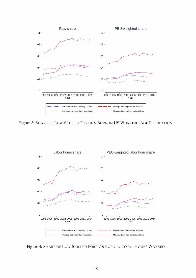
0

.02

.04

.06

.08

.1

1993 1996 1999 2002 2005 2008 2011 2014Year

Raw share

0

.02

.04

.06

.08

.1

1993 1996 1999 2002 2005 2008 2011 2014Year

PEU-weighted share

Foreign-born less than high school Foreign-born high school and less

Mexican-born less than high school Mexican-born high school and less

Figure 3: SHARE OF LOW-SKILLED FOREIGN BORN IN US WORKING-AGE POPULATION

0

.02

.04

.06

.08

.1

1993 1996 1999 2002 2005 2008 2011 2014Year

Labor hours share

0

.02

.04

.06

.08

.1

1993 1996 1999 2002 2005 2008 2011 2014Year

PEU-weighted labor hour share

Foreign-born less than high school Foreign-born high school and less

Mexican-born less than high school Mexican-born high school and less

Figure 4: SHARE OF LOW-SKILLED FOREIGN BORN IN TOTAL HOURS WORKED

48

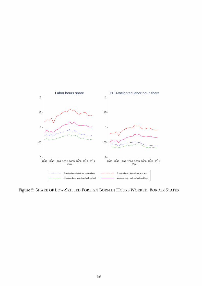
0

.05

.1

.15

.2

1993 1996 1999 2002 2005 2008 2011 2014Year

Labor hours share

0

.05

.1

.15

.2

1993 1996 1999 2002 2005 2008 2011 2014Year

PEU-weighted labor hour share

Foreign-born less than high school Foreign-born high school and less

Mexican-born less than high school Mexican-born high school and less

Figure 5: SHARE OF LOW-SKILLED FOREIGN BORN IN HOURS WORKED, BORDER STATES

49

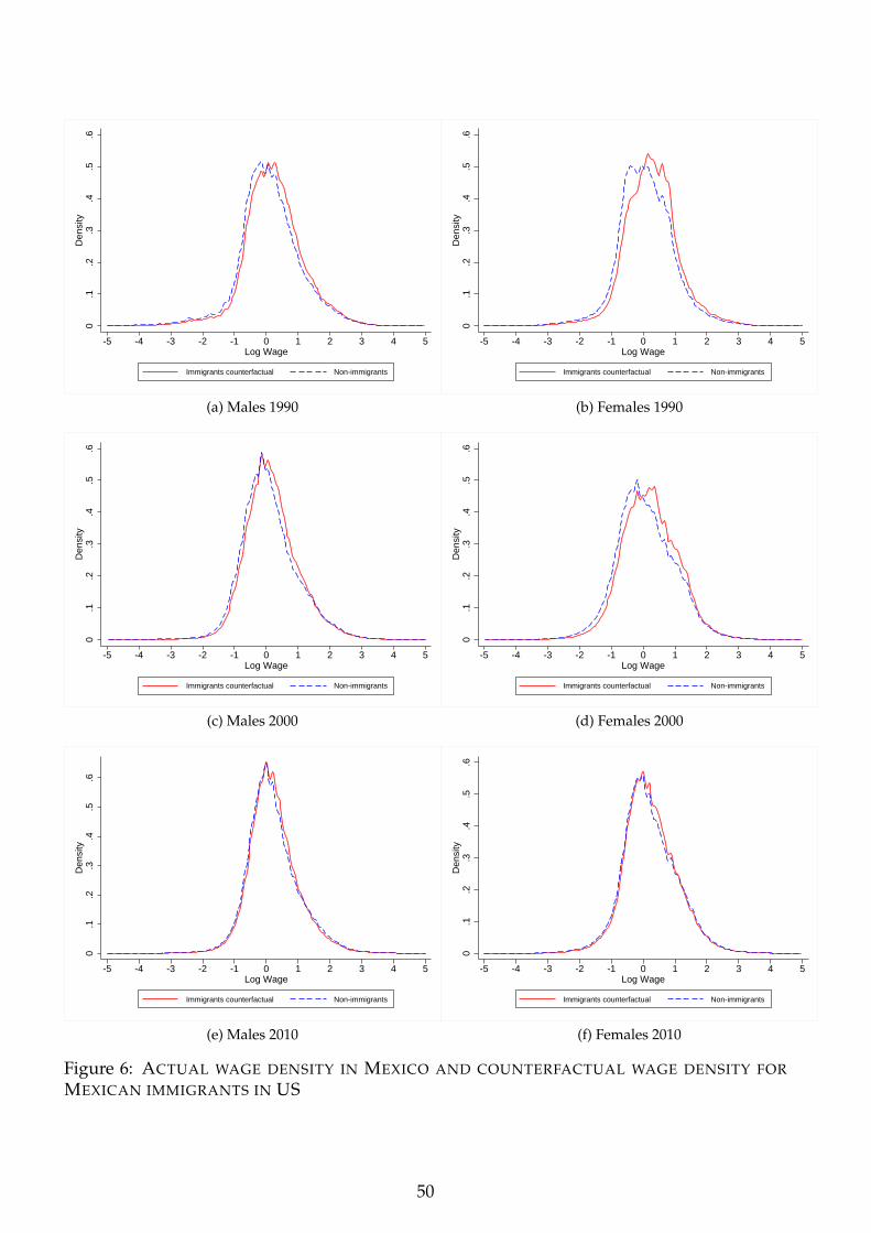
0.1

.2.3

.4.5

.6D

ensi

ty

-5 -4 -3 -2 -1 0 1 2 3 4 5Log Wage

Immigrants counterfactual Non-immigrants

(a) Males 1990

0.1

.2.3

.4.5

.6D

ensi

ty

-5 -4 -3 -2 -1 0 1 2 3 4 5Log Wage

Immigrants counterfactual Non-immigrants

(b) Females 1990

0.1

.2.3

.4.5

.6D

ensi

ty

-5 -4 -3 -2 -1 0 1 2 3 4 5Log Wage

Immigrants counterfactual Non-immigrants

(c) Males 2000

0.1

.2.3

.4.5

.6D

ensi

ty

-5 -4 -3 -2 -1 0 1 2 3 4 5Log Wage

Immigrants counterfactual Non-immigrants

(d) Females 2000

0.1

.2.3

.4.5

.6D

ensi

ty

-5 -4 -3 -2 -1 0 1 2 3 4 5Log Wage

Immigrants counterfactual Non-immigrants

(e) Males 2010

0.1

.2.3

.4.5

.6D

ensi

ty

-5 -4 -3 -2 -1 0 1 2 3 4 5Log Wage

Immigrants counterfactual Non-immigrants

(f) Females 2010

Figure 6: ACTUAL WAGE DENSITY IN MEXICO AND COUNTERFACTUAL WAGE DENSITY FORMEXICAN IMMIGRANTS IN US

50

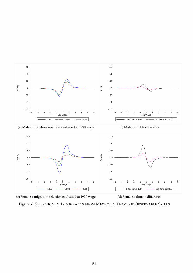
-.15

-.1

-.05

0

.05

.1

.15

Den

sity

-5 -4 -3 -2 -1 0 1 2 3 4 5Log Wage

1990 2000 2010

(a) Males: migration selection evaluated at 1990 wage

-.15

-.1

-.05

0

.05

.1

.15

Den

sity

-5 -4 -3 -2 -1 0 1 2 3 4 5Log Wage

2010 minus 1990 2010 minus 2000

(b) Males: double difference

-.15

-.1

-.05

0

.05

.1

.15

Den

sity

-5 -4 -3 -2 -1 0 1 2 3 4 5Log Wage

1990 2000 2010

(c) Females: migration selection evaluated at 1990 wage

-.15

-.1

-.05

0

.05

.1

.15

Den

sity

-5 -4 -3 -2 -1 0 1 2 3 4 5Log Wage

2010 minus 1990 2010 minus 2000

(d) Females: double difference

Figure 7: SELECTION OF IMMIGRANTS FROM MEXICO IN TERMS OF OBSERVABLE SKILLS

51

(a) Mexico (b) Other Major Sending Countries in Latin America

Figure 8: 50TH PERCENTILE OF INCOME IN SENDING COUNTRY/25TH PERCENTILE OF IN-COME IN US

(a) Mexico (b) Other Major Sending Countries in Latin America

Figure 9: VOLATILITY OF GDP GROWTH (ROLLING 8 QUARTER WINDOWS)

52

0

5000

10000

15000

20000

25000

No.

of o

ffice

rs

1992 1996 2000 2004 2008 2012 2016Year

Southwestern States Nationwide

Figure 10: NUMBER OF U.S. BORDER PATROL AGENTS

Antigua and Barbuda

Bahamas

Barbados Belize

Bolivia

ChileColombia

Costa Rica

DominicanRepublic

Ecuador

ElSalvador

Grenada

Guatemala

Guyana

Haiti

Honduras

Jamaica

Mexico

Nicaragua

Panama

ParaguayPeru

Trinidad & Tobago

Uruguay

Venezuela

050

010

0015

00%

cha

nge

in m

igra

tion

rate

, 198

0-20

15

-50 0 50 100 150% change in birth cohort size, 1980-2015

US Migration Changes on Labor Supply Changes, LAC

Figure 11: US MIGRATION CHANGES ON LABOR SUPPLY CHANGES, LATIN AMERICA ANDCARIBBEAN

53

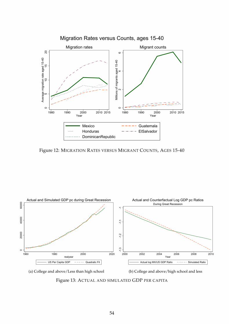
05

1015

20A

vera

ge m

igra

tion

rate

age

d 15

-40

1980 1990 2000 2010 2015Year

Migration rates

02

46

Mill

ions

of m

igra

nts

aged

15-

401980 1990 2000 2010 2015

Year

Migrant counts

Migration Rates versus Counts, ages 15-40

Mexico GuatemalaHonduras ElSalvadorDominicanRepublic

Figure 12: MIGRATION RATES VERSUS MIGRANT COUNTS, AGES 15-40

020

000

4000

060

000

1960 1980 2000 2020realyear

US Per Capita GDP Quadratic Fit

Actual and Simulated GDP pc during Great Recession

(a) College and above/Less than high school

-1.3

-1.2

-1.1

-1

2000 2002 2004 2006 2008 2010Year

Actual log MX/US GDP Ratio Simulated Ratio

During Great RecessionActual and Counterfactual Log GDP pc Ratios

(b) College and above/high school and less

Figure 13: ACTUAL AND SIMULATED GDP PER CAPITA

54

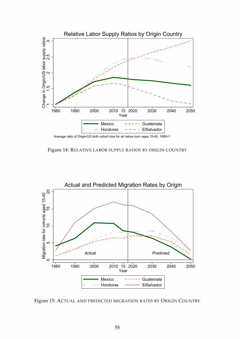
11.

52

2.5

3C

hang

e in

Orig

in/U

S la

bor s

uppl

y ra

tios

1980 1990 2000 2010 15 2020 2030 2040 2050Year

Mexico GuatemalaHonduras ElSalvador

Average ratio of Origin/US birth cohort size for all native born ages 15-40, 1980=1

Relative Labor Supply Ratios by Origin Country

Figure 14: RELATIVE LABOR SUPPLY RATIOS BY ORIGIN COUNTRY

Actual Predicted

05

1015

20M

igra

tion

rate

for c

ohor

ts a

ged

15-4

0

1980 1990 2000 2010 15 2020 2030 2040 2050Year

Mexico GuatemalaHonduras ElSalvador

Actual and Predicted Migration Rates by Origin

Figure 15: ACTUAL AND PREDICTED MIGRATION RATES BY ORIGIN COUNTRY

55

Actual Predicted

02

46

Mill

ions

of m

igra

nts

aged

15-

40

1980 1990 2000 2010 15 2020 2030 2040 2050Year

Mexico GuatemalaHonduras ElSalvador

Stock of Foreign-born Migrants aged 15-40 by Origin

Figure 16: STOCK OF FOREIGN-BORN MIGRANTS AGED 15-40 BY ORIGIN COUNTRY

Figure 17: AGE FREQUENCIES OF MEXICAN-BORN IMMIGRANTS IN US, BY YEAR

56

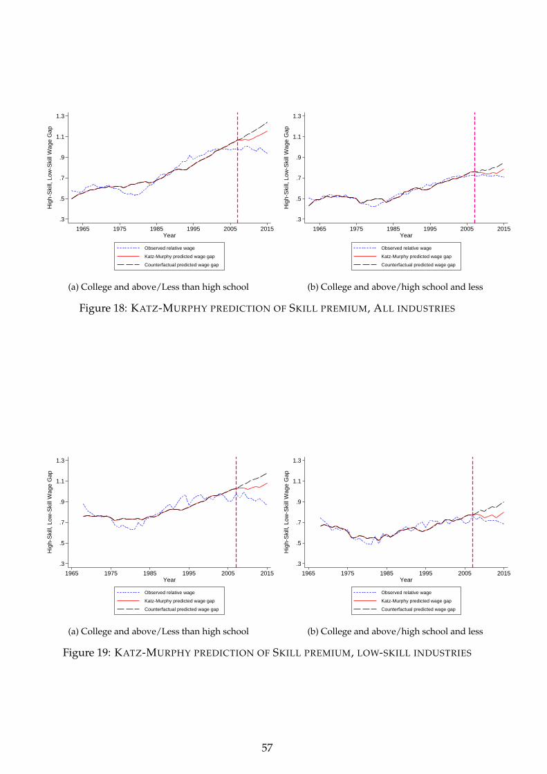
.3

.5

.7

.9

1.1

1.3

Hig

h-S

kill,

Low

-Ski

ll W

age

Gap

1965 1975 1985 1995 2005 2015Year

Observed relative wage

Katz-Murphy predicted wage gap

Counterfactual predicted wage gap

(a) College and above/Less than high school

.3

.5

.7

.9

1.1

1.3

Hig

h-S

kill,

Low

-Ski

ll W

age

Gap

1965 1975 1985 1995 2005 2015Year

Observed relative wage

Katz-Murphy predicted wage gap

Counterfactual predicted wage gap

(b) College and above/high school and less

Figure 18: KATZ-MURPHY PREDICTION OF SKILL PREMIUM, ALL INDUSTRIES

.3

.5

.7

.9

1.1

1.3

Hig

h-S

kill,

Low

-Ski

ll W

age

Gap

1965 1975 1985 1995 2005 2015Year

Observed relative wage

Katz-Murphy predicted wage gap

Counterfactual predicted wage gap

(a) College and above/Less than high school

.3

.5

.7

.9

1.1

1.3

Hig

h-S

kill,

Low

-Ski

ll W

age

Gap

1965 1975 1985 1995 2005 2015Year

Observed relative wage

Katz-Murphy predicted wage gap

Counterfactual predicted wage gap

(b) College and above/high school and less

Figure 19: KATZ-MURPHY PREDICTION OF SKILL PREMIUM, LOW-SKILL INDUSTRIES

57

Table 1: CHARACTERISTICS OF NATIVE-BORN AND FOREIGN-BORN US WORKING-AGEPOPULATION WITH 12 OR FEWER YEARS OF SCHOOLING

1970 1980 1990 2000 2015

NA IM NA IM NA IM NA IM NA IM

MALE 46.4% 41.8% 46.6% 44.4% 48.6% 48.8% 50.3% 51.2% 54.3% 51.2%

MARRIAGE 71.6% 75.8% 63.9% 69.1% 59.1% 64.1% 56.8% 63.9% 46.2% 60.5%

AGE DISTRIBUTION

AGE 18-33 38.1% 28.6% 43.4% 40.2% 41.6% 43.2% 36.4% 42.2% 38.2% 27.3%AGE 34-49 33.5% 34.9% 28.1% 33.0% 31.7% 34.5% 37.9% 38.2% 27.9% 42.3%AGE 50-64 28.5% 36.5% 28.5% 26.8% 26.6% 22.3% 25.6% 19.6% 33.8% 30.5%

YEARS OF SCHOOLING

0-8 23.5% 45.6% 14.3% 39.2% 8.6% 38.2% 4.9% 33.7% 3.98% 29.6%9-11 27.2% 19.6% 24.5% 19.0% 20.8% 16.8% 15.8% 16.5% 12.6% 15.1%12 49.2% 34.8% 61.2% 41.7% 70.6% 45.0% 79.3% 49.8% 83.4% 55.3%

SHARE OF FOREIGN-BORN LABOR FORCE BY TYPE OF ECONOMIC ACTIVITY

AGRICULTURE 3.7% 3.2% 2.9% 4.0% 2.8% 5.7% 2.1% 5.5% 2.3% 6.9%CONSTRUCTION 6.8% 6.1% 6.8% 5.7% 8.0% 7.8% 9.1% 10.8% 9.2% 14.8%EATING, DRINKING ESTABLISHMENTS 2.9% 5.8% 3.8% 6.8% 4.8% 8.7% 5.3% 9.2% 7.6% 11.3%NONDURABLE MANUFACTURE 10.0% 14.5% 8.9% 13.0% 7.6% 9.5% 5.5% 7.5% 4.3% 5.8%PERSONAL SERVICES 4.8% 7.0% 3.2% 5.8% 3.3% 6.9% 2.9% 6.3% 2.9% 7.2%OTHER INDUSTRIES 67.2% 58.7% 66.6% 56.8% 65.2% 51.6% 67.6% 52.1% 63.9% 47.9%UNEMPLOYMENT 4.6% 4.6% 7.8% 7.8% 8.4% 9.8% 7.5% 8.6% 9.7% 6.1%

Notes: Sample is restricted to individuals who are 18-64 years old, and who have 12 years of education orless. NA denotes native-born, and IM denotes foreign-born.

58

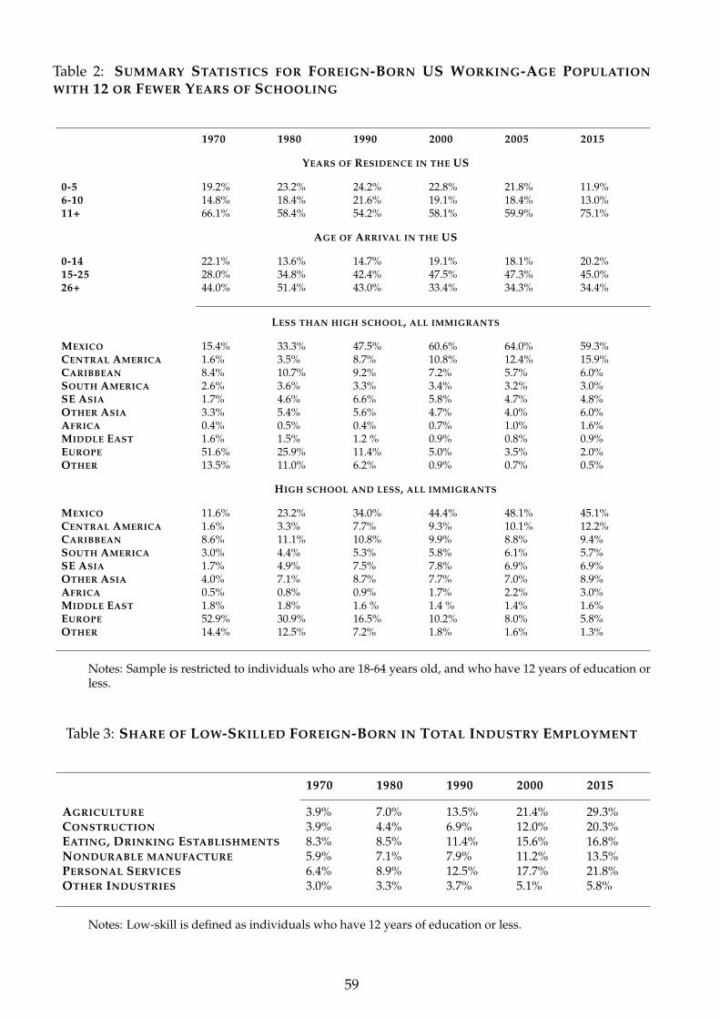
Table 2: SUMMARY STATISTICS FOR FOREIGN-BORN US WORKING-AGE POPULATIONWITH 12 OR FEWER YEARS OF SCHOOLING

1970 1980 1990 2000 2005 2015

YEARS OF RESIDENCE IN THE US

0-5 19.2% 23.2% 24.2% 22.8% 21.8% 11.9%6-10 14.8% 18.4% 21.6% 19.1% 18.4% 13.0%11+ 66.1% 58.4% 54.2% 58.1% 59.9% 75.1%

AGE OF ARRIVAL IN THE US

0-14 22.1% 13.6% 14.7% 19.1% 18.1% 20.2%15-25 28.0% 34.8% 42.4% 47.5% 47.3% 45.0%26+ 44.0% 51.4% 43.0% 33.4% 34.3% 34.4%

LESS THAN HIGH SCHOOL, ALL IMMIGRANTS

MEXICO 15.4% 33.3% 47.5% 60.6% 64.0% 59.3%CENTRAL AMERICA 1.6% 3.5% 8.7% 10.8% 12.4% 15.9%CARIBBEAN 8.4% 10.7% 9.2% 7.2% 5.7% 6.0%SOUTH AMERICA 2.6% 3.6% 3.3% 3.4% 3.2% 3.0%SE ASIA 1.7% 4.6% 6.6% 5.8% 4.7% 4.8%OTHER ASIA 3.3% 5.4% 5.6% 4.7% 4.0% 6.0%AFRICA 0.4% 0.5% 0.4% 0.7% 1.0% 1.6%MIDDLE EAST 1.6% 1.5% 1.2 % 0.9% 0.8% 0.9%EUROPE 51.6% 25.9% 11.4% 5.0% 3.5% 2.0%OTHER 13.5% 11.0% 6.2% 0.9% 0.7% 0.5%

HIGH SCHOOL AND LESS, ALL IMMIGRANTS

MEXICO 11.6% 23.2% 34.0% 44.4% 48.1% 45.1%CENTRAL AMERICA 1.6% 3.3% 7.7% 9.3% 10.1% 12.2%CARIBBEAN 8.6% 11.1% 10.8% 9.9% 8.8% 9.4%SOUTH AMERICA 3.0% 4.4% 5.3% 5.8% 6.1% 5.7%SE ASIA 1.7% 4.9% 7.5% 7.8% 6.9% 6.9%OTHER ASIA 4.0% 7.1% 8.7% 7.7% 7.0% 8.9%AFRICA 0.5% 0.8% 0.9% 1.7% 2.2% 3.0%MIDDLE EAST 1.8% 1.8% 1.6 % 1.4 % 1.4% 1.6%EUROPE 52.9% 30.9% 16.5% 10.2% 8.0% 5.8%OTHER 14.4% 12.5% 7.2% 1.8% 1.6% 1.3%

Notes: Sample is restricted to individuals who are 18-64 years old, and who have 12 years of education orless.

Table 3: SHARE OF LOW-SKILLED FOREIGN-BORN IN TOTAL INDUSTRY EMPLOYMENT

1970 1980 1990 2000 2015

AGRICULTURE 3.9% 7.0% 13.5% 21.4% 29.3%CONSTRUCTION 3.9% 4.4% 6.9% 12.0% 20.3%EATING, DRINKING ESTABLISHMENTS 8.3% 8.5% 11.4% 15.6% 16.8%NONDURABLE MANUFACTURE 5.9% 7.1% 7.9% 11.2% 13.5%PERSONAL SERVICES 6.4% 8.9% 12.5% 17.7% 21.8%OTHER INDUSTRIES 3.0% 3.3% 3.7% 5.1% 5.8%

Notes: Low-skill is defined as individuals who have 12 years of education or less.

59

Table 4: ANALYSIS OF NET MIGRATION AT MEXICAN STATE LEVEL

(1) (2) (3) (4)

Dependent variable: Decennial change in net migration Base IV Excluding 2010 Men Women

Log Ratio of MX state to US HS Dropout labor supply 0.1441*** 0.1643*** 0.1733*** 0.1190***(0.010) (0.011) (0.015) (0.013)

Log innovations to MX state/US GDP pc at age 16 -0.0197* -0.0735*** -0.0262 -0.0134(0.010) (0.016) (0.017) (0.012)

Log innovations to MX state/US GDP pc in census year 0.022 -0.0472 0.0234 0.0187(0.020) (0.039) (0.034) (0.024)

Observations 3,328 2,432 1,664 1,664R-squared 0.112 0.175 0.108 0.189

Notes: Unit of analysis is the three-year Mexican state/gender birth cohort. Mexican state cohort size is fixed at its initial value; thenumber of native US high school dropouts is contemporaneous. GDP refers to GDP per capita. In IV regressions, log (MX state birthcohort size/ US birth cohort size) is used as an instrument for log (MX state birth cohort size/US HS dropouts). Regressions in alltables use robust SEs clustered at the cohort level and are weighted by birth cohort size. Standard errors in parentheses, * significantat 10%; ** significant at 5%, ***significant at 1%.

60

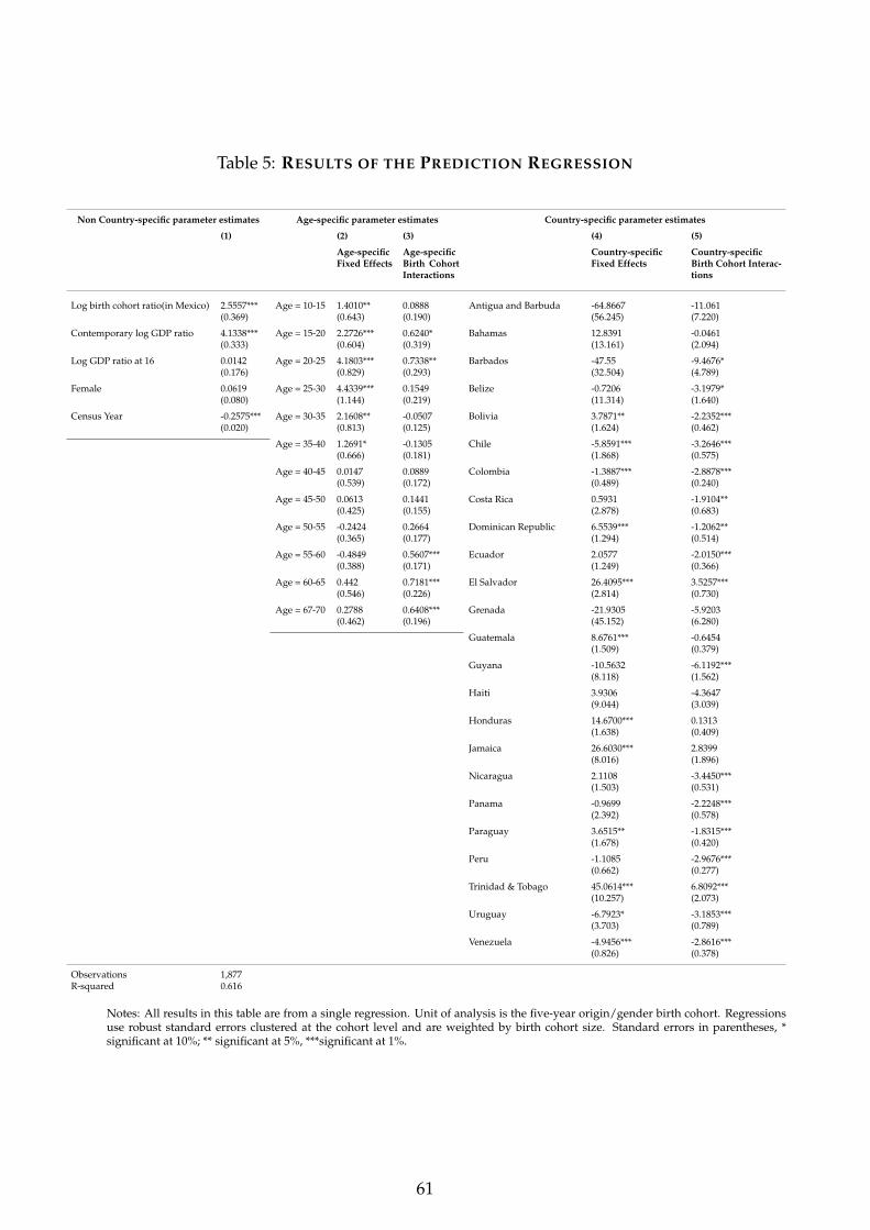
Table 5: RESULTS OF THE PREDICTION REGRESSION

Non Country-specific parameter estimates Age-specific parameter estimates Country-specific parameter estimates

(1) (2) (3) (4) (5)

Age-specificFixed Effects

Age-specificBirth CohortInteractions

Country-specificFixed Effects

Country-specificBirth Cohort Interac-tions

Log birth cohort ratio(in Mexico) 2.5557*** Age = 10-15 1.4010** 0.0888 Antigua and Barbuda -64.8667 -11.061(0.369) (0.643) (0.190) (56.245) (7.220)

Contemporary log GDP ratio 4.1338*** Age = 15-20 2.2726*** 0.6240* Bahamas 12.8391 -0.0461(0.333) (0.604) (0.319) (13.161) (2.094)

Log GDP ratio at 16 0.0142 Age = 20-25 4.1803*** 0.7338** Barbados -47.55 -9.4676*(0.176) (0.829) (0.293) (32.504) (4.789)

Female 0.0619 Age = 25-30 4.4339*** 0.1549 Belize -0.7206 -3.1979*(0.080) (1.144) (0.219) (11.314) (1.640)

Census Year -0.2575*** Age = 30-35 2.1608** -0.0507 Bolivia 3.7871** -2.2352***(0.020) (0.813) (0.125) (1.624) (0.462)

Age = 35-40 1.2691* -0.1305 Chile -5.8591*** -3.2646***(0.666) (0.181) (1.868) (0.575)

Age = 40-45 0.0147 0.0889 Colombia -1.3887*** -2.8878***(0.539) (0.172) (0.489) (0.240)

Age = 45-50 0.0613 0.1441 Costa Rica 0.5931 -1.9104**(0.425) (0.155) (2.878) (0.683)

Age = 50-55 -0.2424 0.2664 Dominican Republic 6.5539*** -1.2062**(0.365) (0.177) (1.294) (0.514)

Age = 55-60 -0.4849 0.5607*** Ecuador 2.0577 -2.0150***(0.388) (0.171) (1.249) (0.366)

Age = 60-65 0.442 0.7181*** El Salvador 26.4095*** 3.5257***(0.546) (0.226) (2.814) (0.730)

Age = 67-70 0.2788 0.6408*** Grenada -21.9305 -5.9203(0.462) (0.196) (45.152) (6.280)

Guatemala 8.6761*** -0.6454(1.509) (0.379)

Guyana -10.5632 -6.1192***(8.118) (1.562)

Haiti 3.9306 -4.3647(9.044) (3.039)

Honduras 14.6700*** 0.1313(1.638) (0.409)

Jamaica 26.6030*** 2.8399(8.016) (1.896)

Nicaragua 2.1108 -3.4450***(1.503) (0.531)

Panama -0.9699 -2.2248***(2.392) (0.578)

Paraguay 3.6515** -1.8315***(1.678) (0.420)

Peru -1.1085 -2.9676***(0.662) (0.277)

Trinidad & Tobago 45.0614*** 6.8092***(10.257) (2.073)

Uruguay -6.7923* -3.1853***(3.703) (0.789)

Venezuela -4.9456*** -2.8616***(0.826) (0.378)

Observations 1,877R-squared 0.616

Notes: All results in this table are from a single regression. Unit of analysis is the five-year origin/gender birth cohort. Regressionsuse robust standard errors clustered at the cohort level and are weighted by birth cohort size. Standard errors in parentheses, *significant at 10%; ** significant at 5%, ***significant at 1%.

61

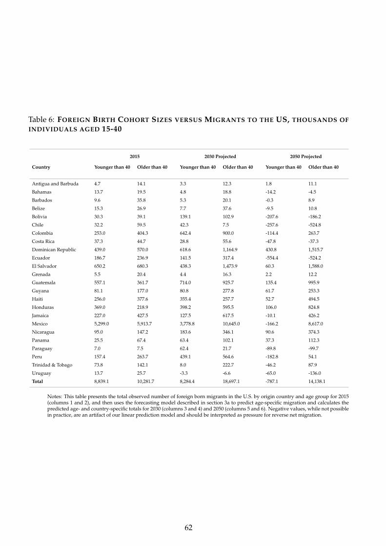
Table 6: FOREIGN BIRTH COHORT SIZES VERSUS MIGRANTS TO THE US, THOUSANDS OFINDIVIDUALS AGED 15-40

2015 2030 Projected 2050 Projected

Country Younger than 40 Older than 40 Younger than 40 Older than 40 Younger than 40 Older than 40

Antigua and Barbuda 4.7 14.1 3.3 12.3 1.8 11.1

Bahamas 13.7 19.5 4.8 18.8 -14.2 -4.5

Barbados 9.6 35.8 5.3 20.1 -0.3 8.9

Belize 15.3 26.9 7.7 37.6 -9.5 10.8

Bolivia 30.3 39.1 139.1 102.9 -207.6 -186.2

Chile 32.2 59.5 42.3 7.5 -257.6 -524.8

Colombia 253.0 404.3 642.4 900.0 -114.4 263.7

Costa Rica 37.3 44.7 28.8 55.6 -47.8 -37.3

Dominican Republic 439.0 570.0 618.6 1,164.9 430.8 1,515.7

Ecuador 186.7 236.9 141.5 317.4 -554.4 -524.2

El Salvador 650.2 680.3 438.3 1,473.9 60.3 1,588.0

Grenada 5.5 20.4 4.4 16.3 2.2 12.2

Guatemala 557.1 361.7 714.0 925.7 135.4 995.9

Guyana 81.1 177.0 80.8 277.8 61.7 253.3

Haiti 256.0 377.6 355.4 257.7 52.7 494.5

Honduras 369.0 218.9 398.2 595.5 106.0 824.8

Jamaica 227.0 427.5 127.5 617.5 -10.1 426.2

Mexico 5,299.0 5,913.7 3,778.8 10,645.0 -166.2 8,617.0

Nicaragua 95.0 147.2 183.6 346.1 90.6 374.3

Panama 25.5 67.4 63.4 102.1 37.3 112.3

Paraguay 7.0 7.5 62.4 21.7 -89.8 -99.7

Peru 157.4 263.7 439.1 564.6 -182.8 54.1

Trinidad & Tobago 73.8 142.1 8.0 222.7 -46.2 87.9

Uruguay 13.7 25.7 -3.3 -6.6 -65.0 -136.0

Total 8,839.1 10,281.7 8,284.4 18,697.1 -787.1 14,138.1

Notes: This table presents the total observed number of foreign born migrants in the U.S. by origin country and age group for 2015(columns 1 and 2), and then uses the forecasting model described in section 3a to predict age-specific migration and calculates thepredicted age- and country-specific totals for 2030 (columns 3 and 4) and 2050 (columns 5 and 6). Negative values, while not possiblein practice, are an artifact of our linear prediction model and should be interpreted as pressure for reverse net migration.

62