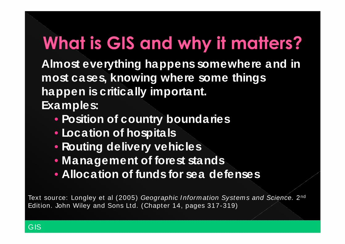
Almost everything happens somewhere and in most cases, knowing where some things happen is critically important. Examples:

• Position of country boundaries• Location of hospitals• Routing delivery vehicles• Management of forest stands• Allocation of funds for sea defenses

Text source: Longley et al (2005) Geographic Information Systems and Science. 2nd

Edition. John Wiley and Sons Ltd. (Chapter 14, pages 317-319)

GIS

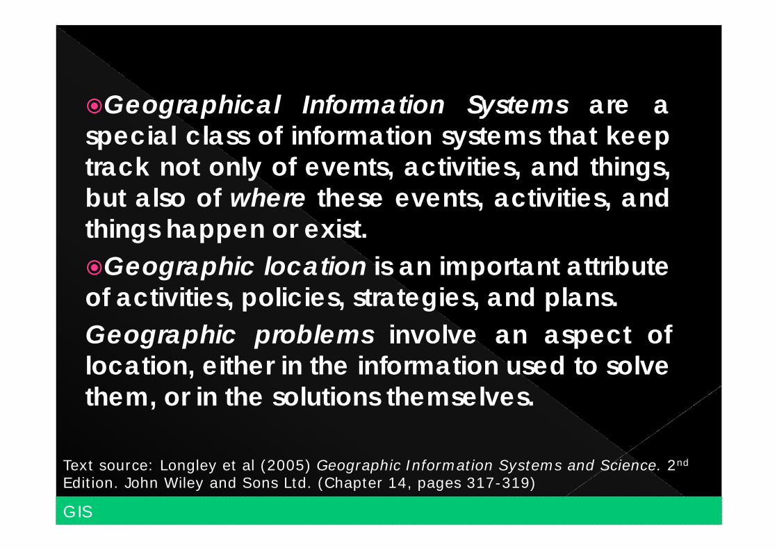
Geographical Information Systems are aspecial class of information systems that keeptrack not only of events, activities, and things,but also of where these events, activities, andthings happen or exist.Geographic location is an important attributeof activities, policies, strategies, and plans.Geographic problems involve an aspect oflocation, either in the information used to solvethem, or in the solutions themselves.

3GIS

Text source: Longley et al (2005) Geographic Information Systems and Science. 2nd

Edition. John Wiley and Sons Ltd. (Chapter 14, pages 317-319)

4GIS

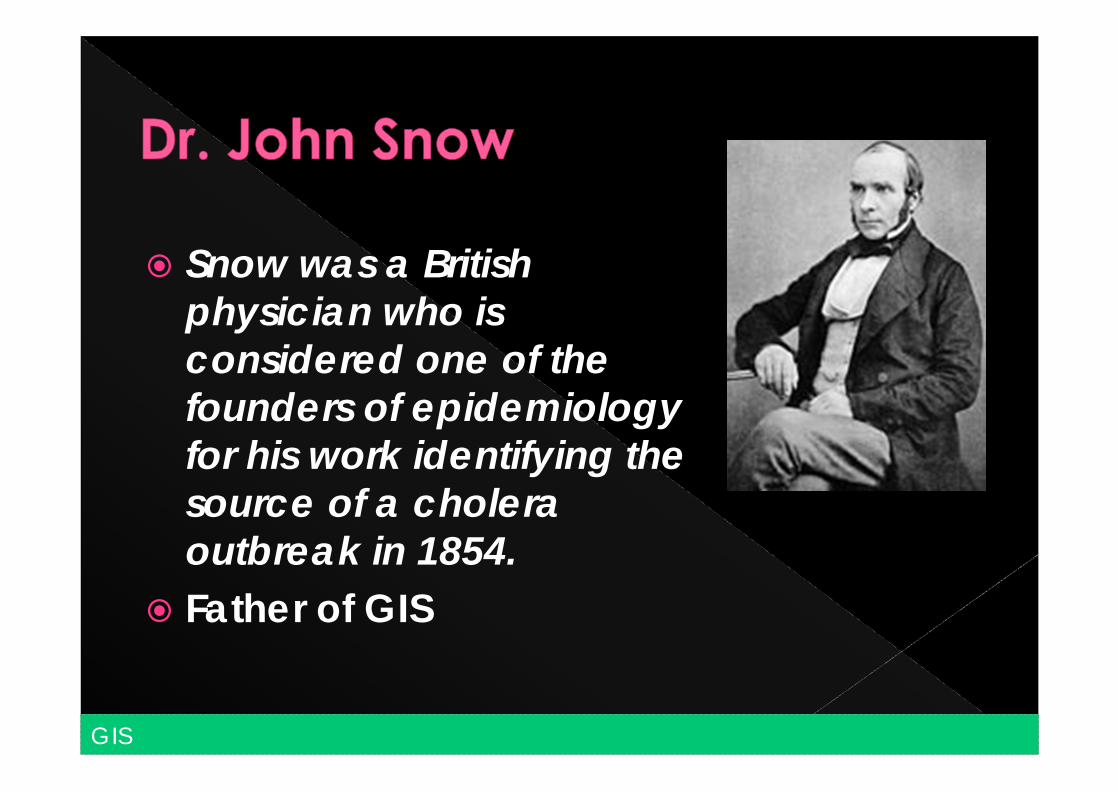
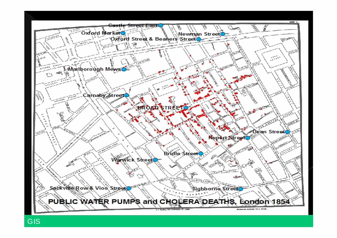
Snow was a British physician who is considered one of the founders of epidemiology for his work identifying the source of a cholera outbreak in 1854.

Father of GIS

5GIS

6GIS

I. IntroductionII. Objectives of the StudyIII. Study AreaIV. MethodologyV. ResultsVI. Conclusions and Further Studies

7

The 2009 EFA Global MonitoringReport (UNESCO 2008) listed thePhilippines as one of the countrieswith decreased enrolment rate from 1999to 2006 having more than 500,000 outof school children. This trend ineducation indicators for monitoring thesecond MDG suggests that the countrymay probably not meet its target by2015.

8Introduction

Cohort Survival Rates (CSR*) for the past10 years have fluctuated between 60 %and 80 % in both elementary andsecondary levels (Department ofEducation, 2008).

This is alarming; education is a pre-condition to a country’s long-termeconomic growth (IIASA, 2008)

9Introduction

*the percentage of enrolees at the beginning grade or year in a given school year who reached the final grade or year of the elementary/secondary level

10

Tanauan City has been improving the quality of education from pre-school to high school.

As of 2009 there are already a total of 44 public elementary schools and 12 public secondary schools in the city. There are also 35 private educational institutions operating which caters elementary or secondary education or both.

11

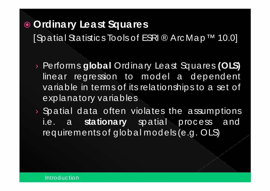
Ordinary Least Squares[Spatial Statistics Tools of ESRI ® ArcMap™ 10.0]

› Performs global Ordinary Least Squares (OLS)linear regression to model a dependentvariable in terms of its relationships to a set ofexplanatory variables

› Spatial data often violates the assumptionsi.e. a stationary spatial process andrequirements of global models (e.g. OLS)

12Introduction

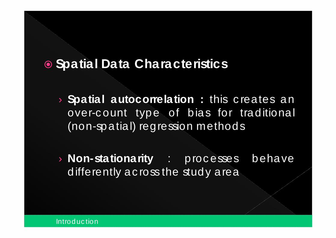
Spatial Data Characteristics

› Spatial autocorrelation : this creates anover-count type of bias for traditional(non-spatial) regression methods

› Non-stationarity : processes behavedifferently across the study area

13Introduction

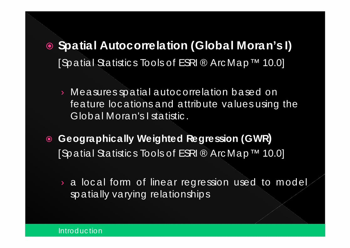
Spatial Autocorrelation (Global Moran’s I)[Spatial Statistics Tools of ESRI ® ArcMap™ 10.0]

› Measures spatial autocorrelation based on feature locations and attribute values using the Global Moran's I statistic.

14Introduction

Geographically Weighted Regression (GWR)[Spatial Statistics Tools of ESRI ® ArcMap™ 10.0]

› a local form of linear regression used to modelspatially varying relationships

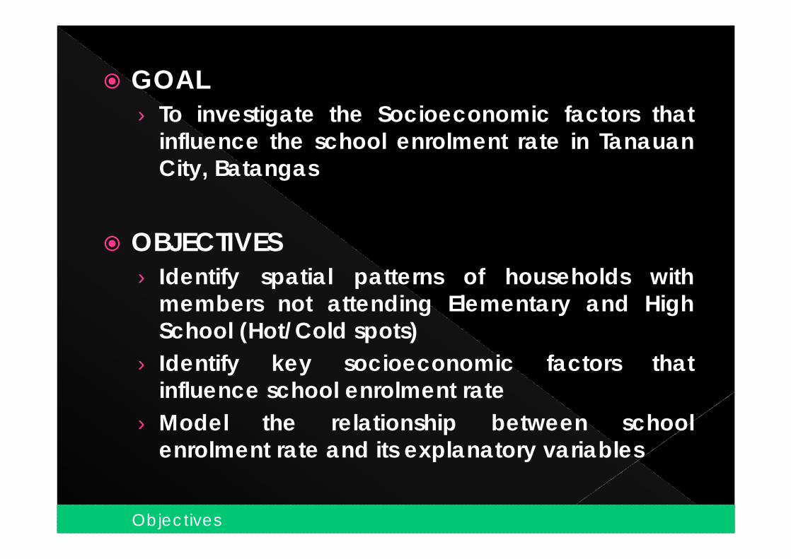
GOAL› To investigate the Socioeconomic factors that

influence the school enrolment rate in TanauanCity, Batangas

OBJECTIVES› Identify spatial patterns of households with

members not attending Elementary and HighSchool (Hot/Cold spots)

› Identify key socioeconomic factors thatinfluence school enrolment rate

› Model the relationship between schoolenrolment rate and its explanatory variables

15Objectives

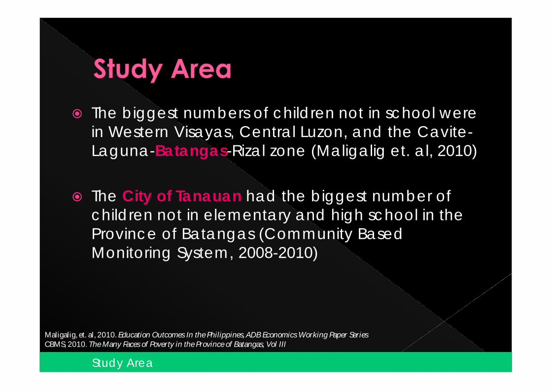
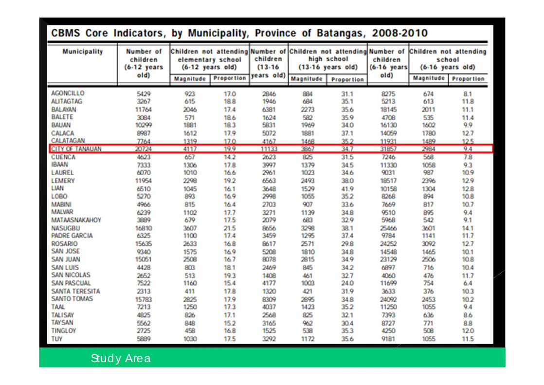
The biggest numbers of children not in school were in Western Visayas, Central Luzon, and the Cavite-Laguna-Batangas-Rizal zone (Maligalig et. al, 2010)

The City of Tanauan had the biggest number of children not in elementary and high school in the Province of Batangas (Community Based Monitoring System, 2008-2010)

16Study Area

Maligalig, et. al, 2010. Education Outcomes In the Philippines, ADB Economics Working Paper SeriesCBMS, 2010. The Many Faces of Poverty in the Province of Batangas, Vol III

17

18

Natural Attractions

19

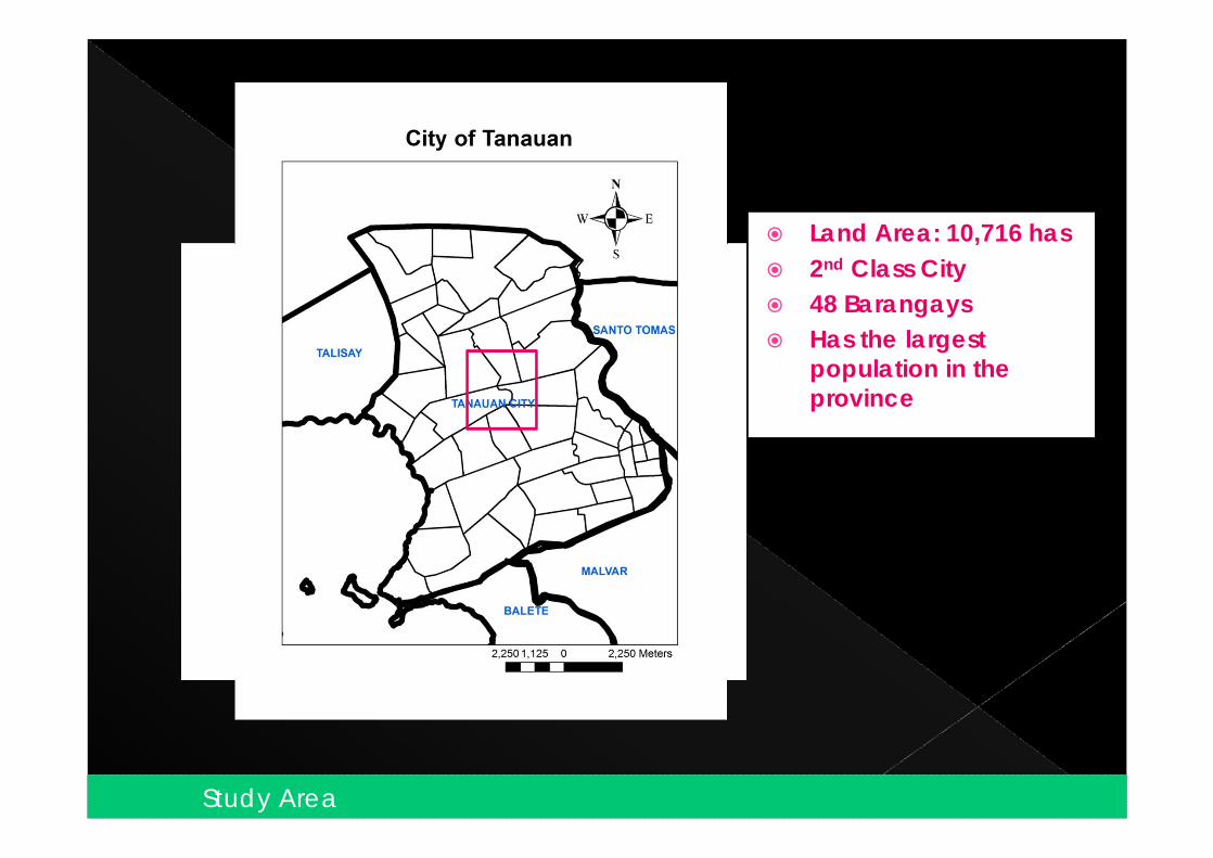
Land Area: 10,716 has 2nd Class City 48 Barangays Has the largest

population in the province

20Study Area

21Study Area

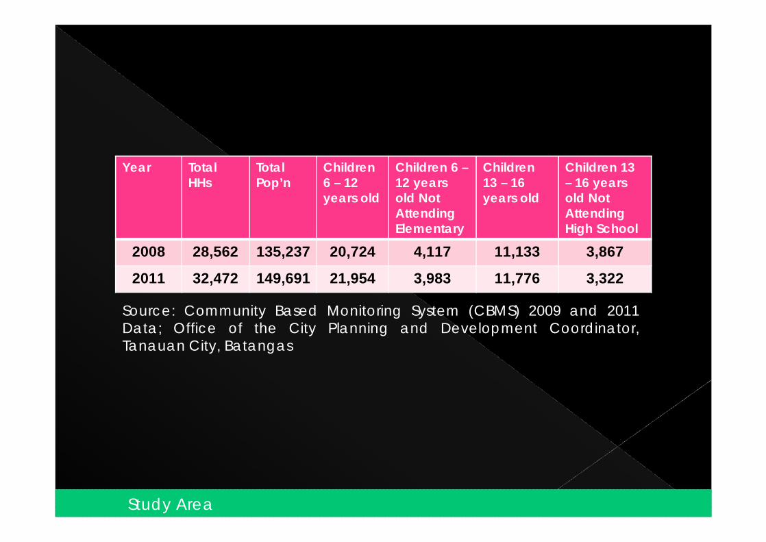
Year Total HHs

Total Pop’n

Children 6 – 12 years old

Children 6 –12 years old Not Attending Elementary

Children 13 – 16 years old

Children 13 – 16 years old Not Attending High School

2008 28,562 135,237 20,724 4,117 11,133 3,867

2011 32,472 149,691 21,954 3,983 11,776 3,322

Source: Community Based Monitoring System (CBMS) 2009 and 2011Data; Office of the City Planning and Development Coordinator,Tanauan City, Batangas

22Study Area

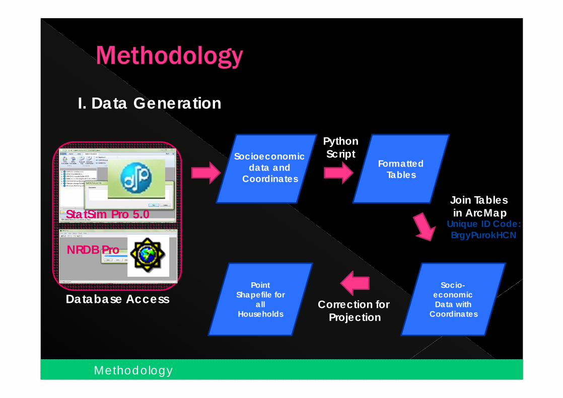
StatSim Pro 5.0

NRDB Pro

Database Access

23

Socioeconomic data and

Coordinates

Unique ID Code: BrgyPurokHCN

Formatted Tables

Python Script

Join Tablesin ArcMap

Socio-economic Data with

Coordinates

Point Shapefile for

all Households

Correction for Projection

I. Data Generation

Methodology

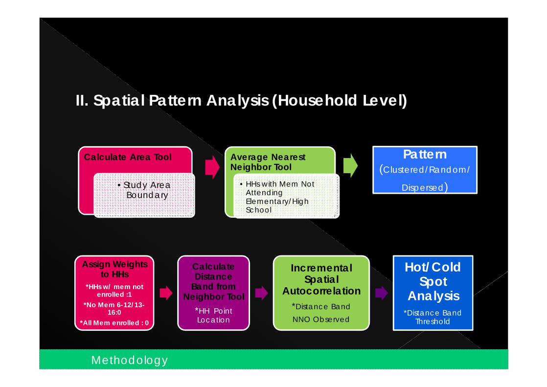
II. Spatial Pattern Analysis (Household Level)

Calculate Area Tool

•Study Area Boundary

Average Nearest Neighbor Tool

• HHs with Mem Not Attending Elementary/High School

Pattern (Clustered/Random/

Dispersed)

Assign Weights to HHs

*HHs w/ mem not enrolled :1

*No Mem 6-12/13-16:0

*All Mem enrolled : 0

Calculate Distance

Band from Neighbor Tool

*HH Point Location

Incremental Spatial

Autocorrelation*Distance BandNNO Observed

Hot/Cold Spot

Analysis*Distance Band

Threshold

24Methodology

III. Spatial Regression Analysis (Barangay Level)

25

Y = ß0+ ß1X1 + ß2X2 +… ßnXn + ε

Factor3

Factor10

Factor1

Factor6

Factor7

Factor8

Factor9

Factor4

Factor2Factor5

Scatter Plot Matrix and R-squared

Initially Identified

Explanatory Variables

OLS Summary & Diagnostics

Dependent Variable

EV4

EV3

EV2

EV1

EV6

EV5

Key Variables

GWR

OLS

Yi = ßi0+ ßi1X1 + ßi2X2+… ßinXn + ε

Global Model

Local Model

Methodology

Diagnostics

- Coefficient Determination- AkaikeInformation Criterion (AICc)- Adjusted R-squared- Joint F Statistic- Wald Statistic- Variance Inflation Factor (VIF)- Koenker’sBreusch-Pagan statistic- Jarque-Berastatistic

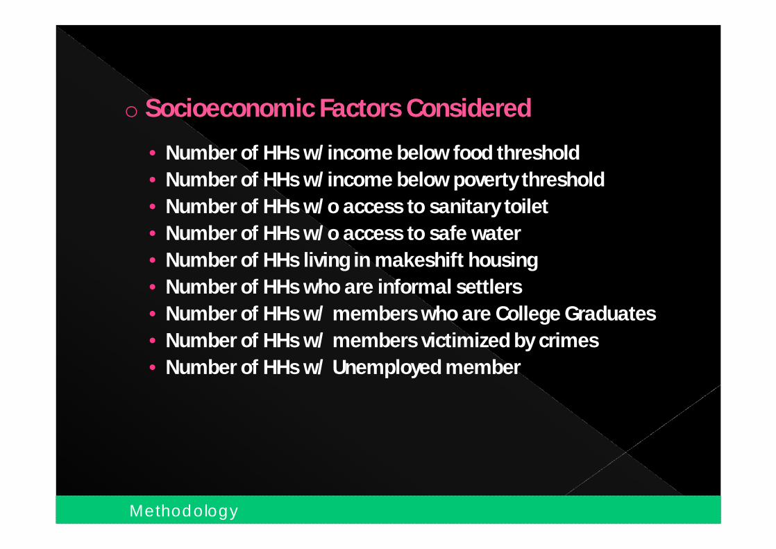
o Socioeconomic Factors Considered

• Number of HHs w/income below food threshold• Number of HHs w/income below poverty threshold• Number of HHs w/o access to sanitary toilet• Number of HHs w/o access to safe water• Number of HHs living in makeshift housing• Number of HHs who are informal settlers• Number of HHs w/ members who are College Graduates• Number of HHs w/ members victimized by crimes• Number of HHs w/ Unemployed member

26Methodology

27

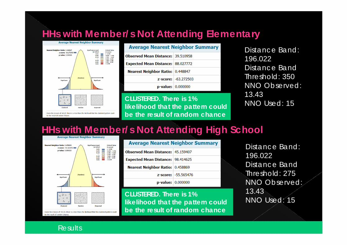
HHs with Member/s Not Attending Elementary

HHs with Member/s Not Attending High School

CLUSTERED. There is 1% likelihood that the pattern could be the result of random chance

CLUSTERED. There is 1% likelihood that the pattern could be the result of random chance

Distance Band: 196.022Distance Band Threshold: 350NNO Observed: 13.43NNO Used: 15

Distance Band: 196.022Distance Band Threshold: 275NNO Observed: 13.43NNO Used: 15

28Results

29Results

30

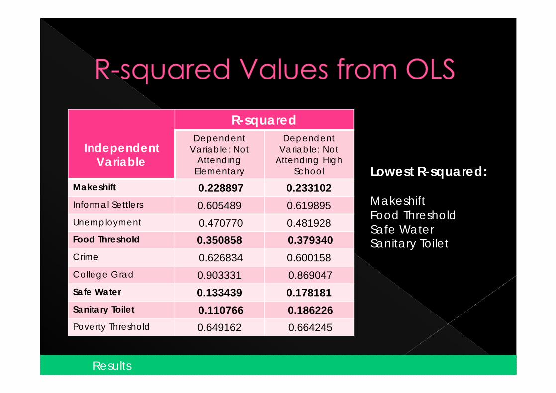
Independent Variable

R-squaredDependent

Variable: Not Attending

Elementary

Dependent Variable: Not

Attending High School

Makeshift 0.228897 0.233102 Informal Settlers 0.605489 0.619895Unemployment 0.470770 0.481928Food Threshold 0.350858 0.379340Crime 0.626834 0.600158 College Grad 0.903331 0.869047 Safe Water 0.133439 0.178181Sanitary Toilet 0.110766 0.186226Poverty Threshold 0.649162 0.664245

Lowest R-squared:

MakeshiftFood ThresholdSafe WaterSanitary Toilet

Results

31Results

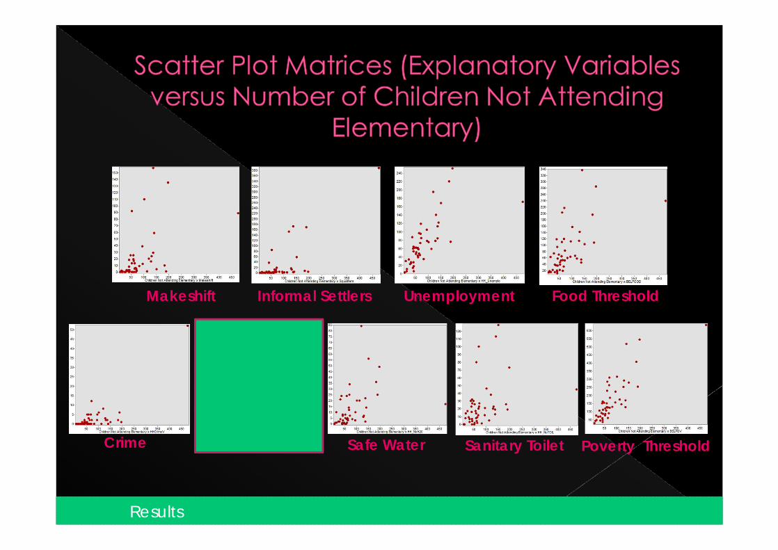
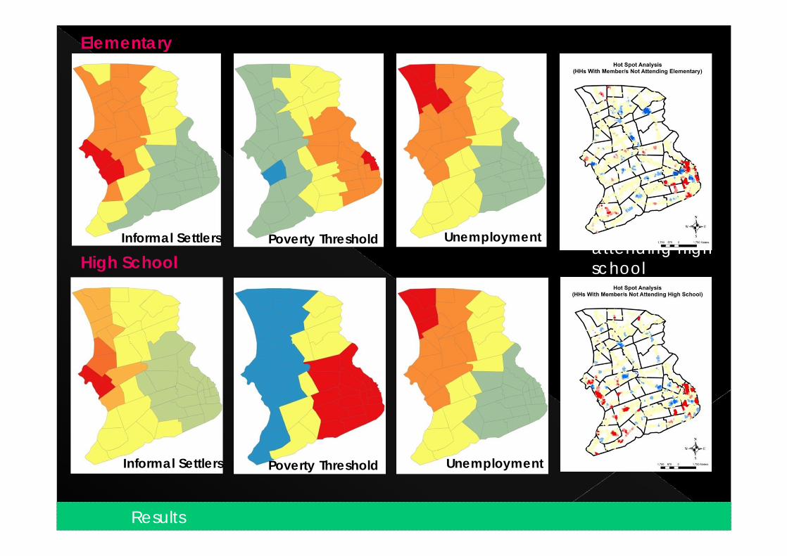
Makeshift Informal Settlers Unemployment Food Threshold

Crime College Grad Poverty ThresholdSanitary ToiletSafe Water

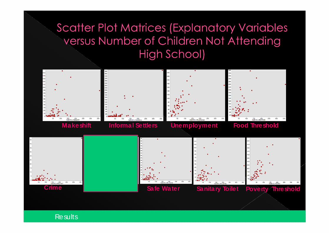
32Results

Makeshift Informal Settlers Unemployment Food Threshold

Crime College Grad Poverty ThresholdSanitary ToiletSafe Water

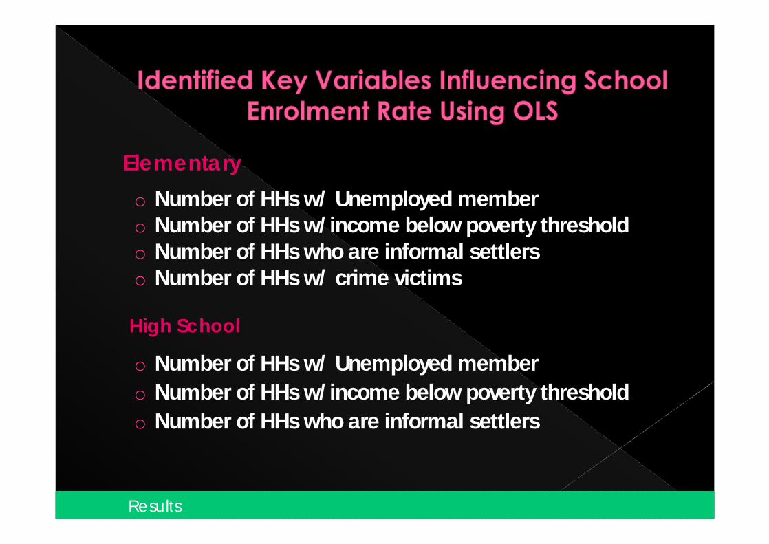
o Number of HHs w/ Unemployed membero Number of HHs w/income below poverty thresholdo Number of HHs who are informal settlerso Number of HHs w/ crime victims

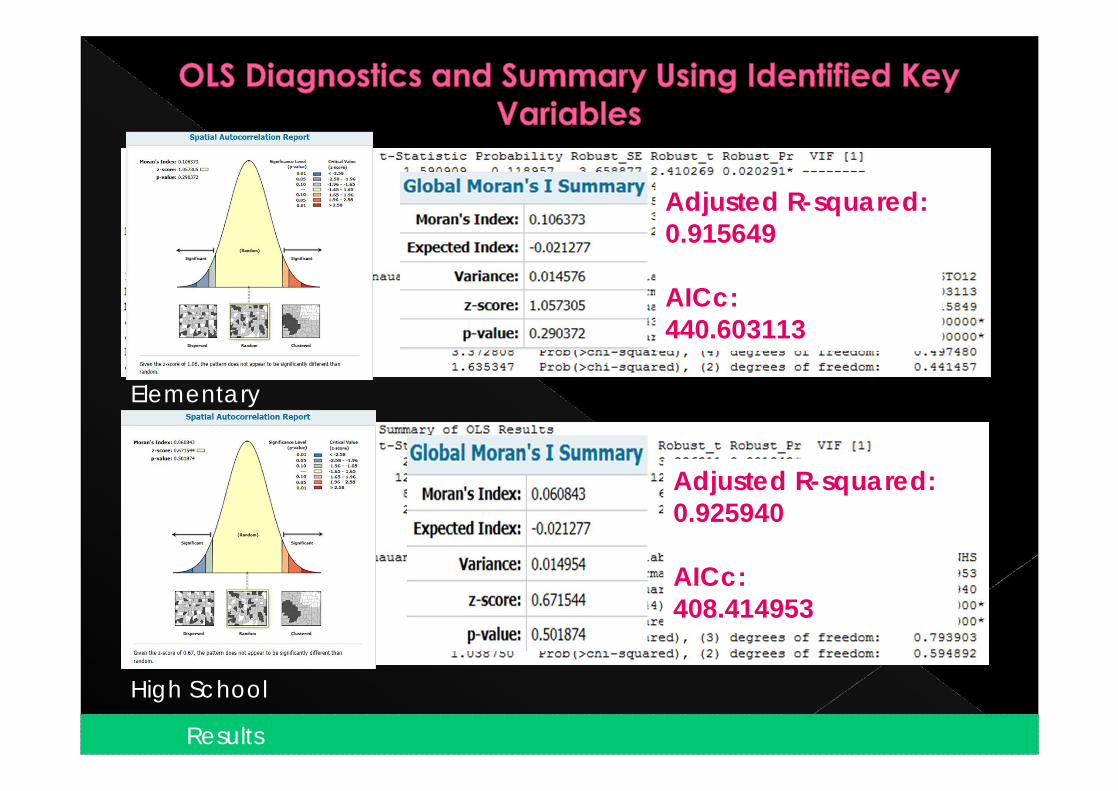
33Results

Elementary

High School

o Number of HHs w/ Unemployed membero Number of HHs w/income below poverty thresholdo Number of HHs who are informal settlers

34

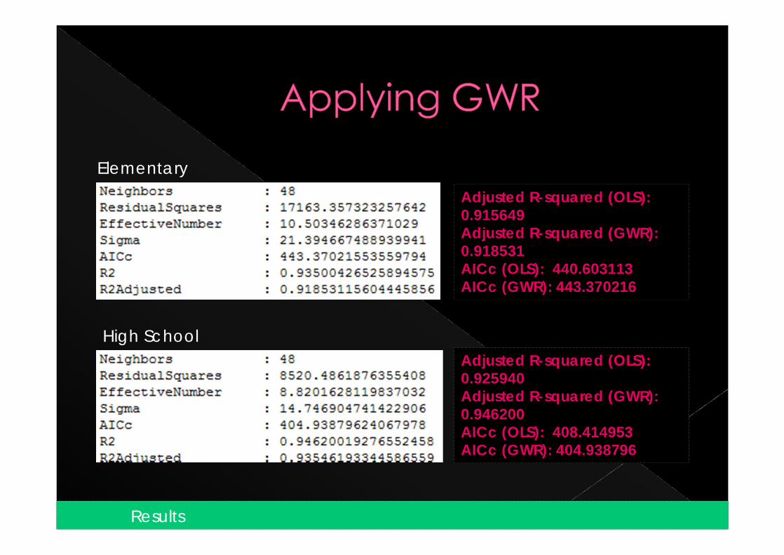
Adjusted R-squared: 0.915649

AICc: 440.603113

Elementary

High School

Adjusted R-squared: 0.925940

AICc: 408.414953

Results

35

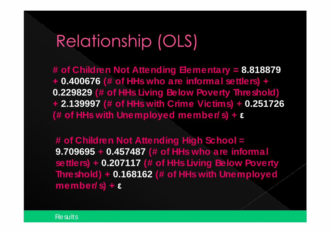
# of Children Not Attending Elementary = 8.818879+ 0.400676 (# of HHs who are informal settlers) + 0.229829 (# of HHs Living Below Poverty Threshold) + 2.139997 (# of HHs with Crime Victims) + 0.251726(# of HHs with Unemployed member/s) + ε

# of Children Not Attending High School = 9.709695 + 0.457487 (# of HHs who are informal settlers) + 0.207117 (# of HHs Living Below Poverty Threshold) + 0.168162 (# of HHs with Unemployed member/s) + ε

Results

36

Elementary

High School

Adjusted R-squared (OLS): 0.915649Adjusted R-squared (GWR):0.918531AICc (OLS): 440.603113AICc (GWR): 443.370216

Adjusted R-squared (OLS): 0.925940Adjusted R-squared (GWR):0.946200AICc (OLS): 408.414953AICc (GWR): 404.938796

Results

37Results

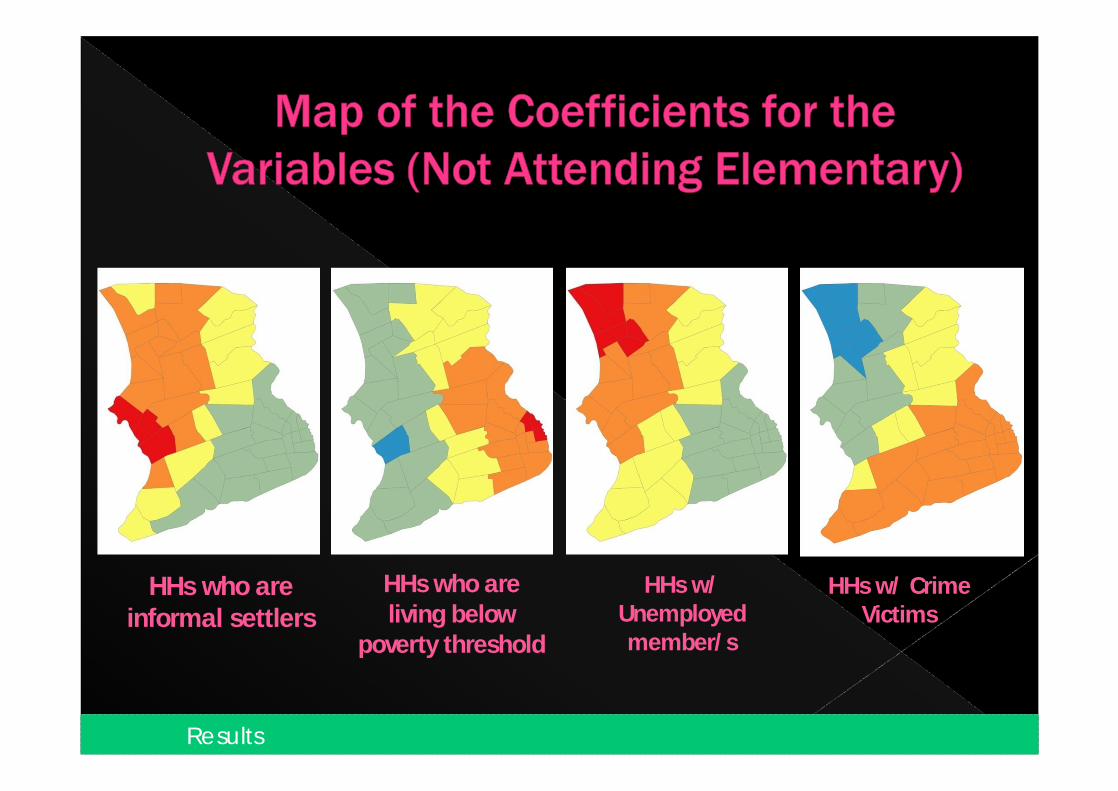
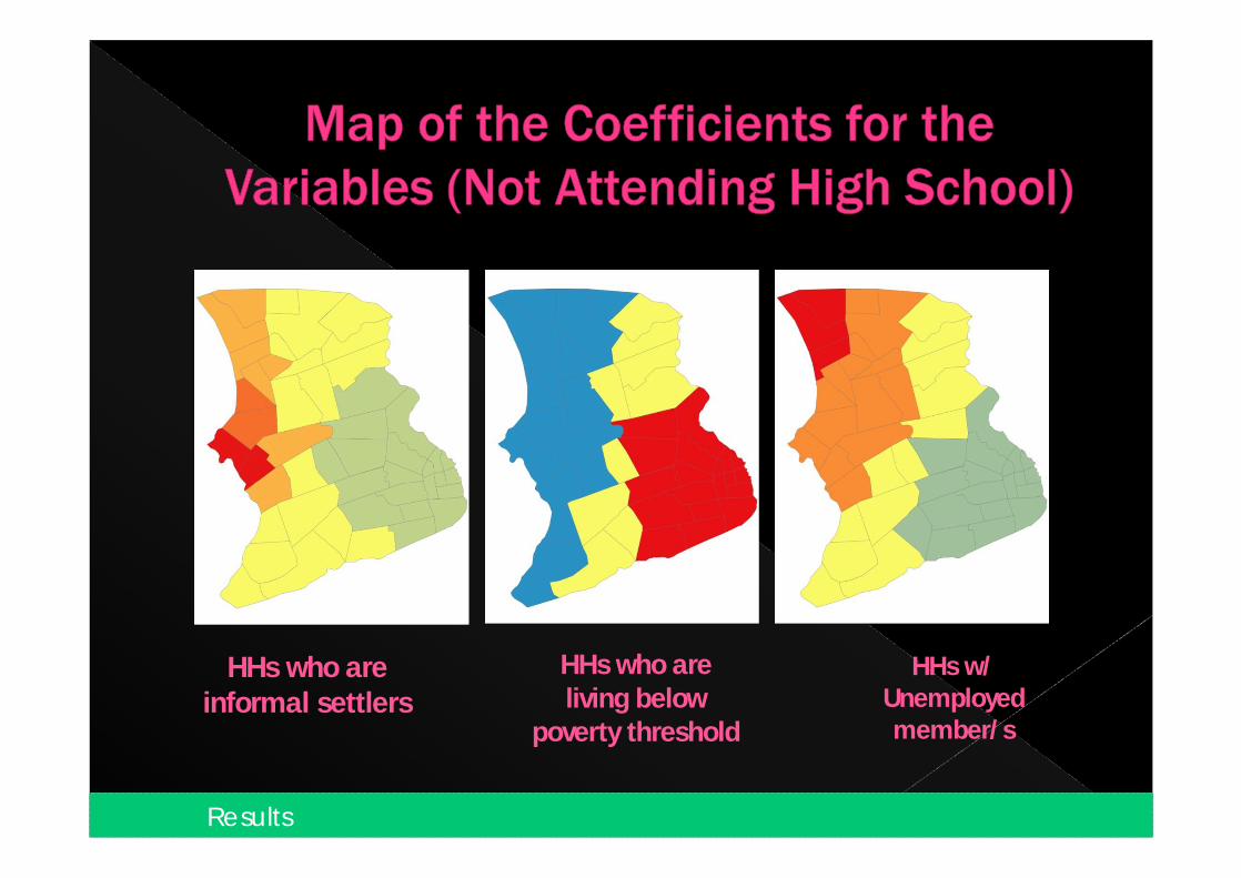
HHs who are informal settlers

HHs who are living below

poverty threshold

HHs w/ Unemployed member/s

HHs w/ Crime Victims

38Results

39

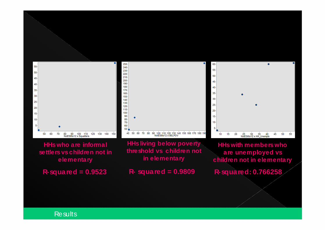
HHs living below poverty threshold vs children not

in elementary

R-squared: 0.766258R-squared = 0.9523

HHs who are informal settlers vs children not in

elementary

HHs with members who are unemployed vs

children not in elementary

R- squared = 0.9809

Results

40

HHs who are informal settlers

HHs who are living below

poverty threshold

HHs w/ Unemployed member/s

Results

41

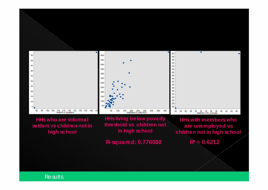
R-squared: 0.776088 R² = 0.6212

HHs living below poverty threshold vs children not

in high school

HHs who are informal settlers vs children not in

high school

HHs with members who are unemployed vs

children not in high school

Results

42Results

Elementary

High School

HHs Living Below Poverty Threshold is a stronger predictor for the number of children not attending high school compared to the number of children not attending elementary in most of the barangays in the east.

Informal Settlers

Informal Settlers

Poverty Threshold

Poverty Threshold Unemployment

Unemployment

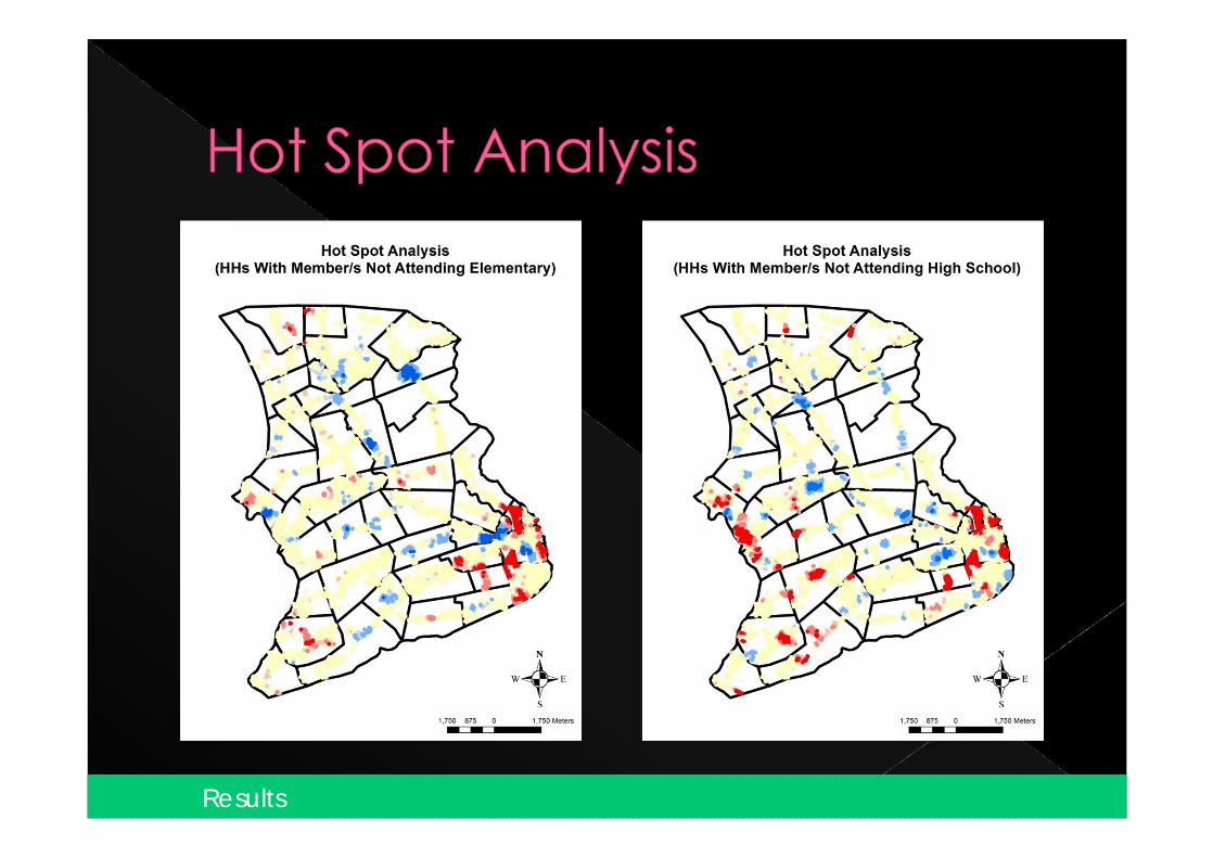
The Poblacion-DarasaArea is a hot spot for both HHs with member/s not attending Elementary and High School

The barangays near the Taal Lake are also hot spots for HHs with member/s not attending High School

43Conclusions

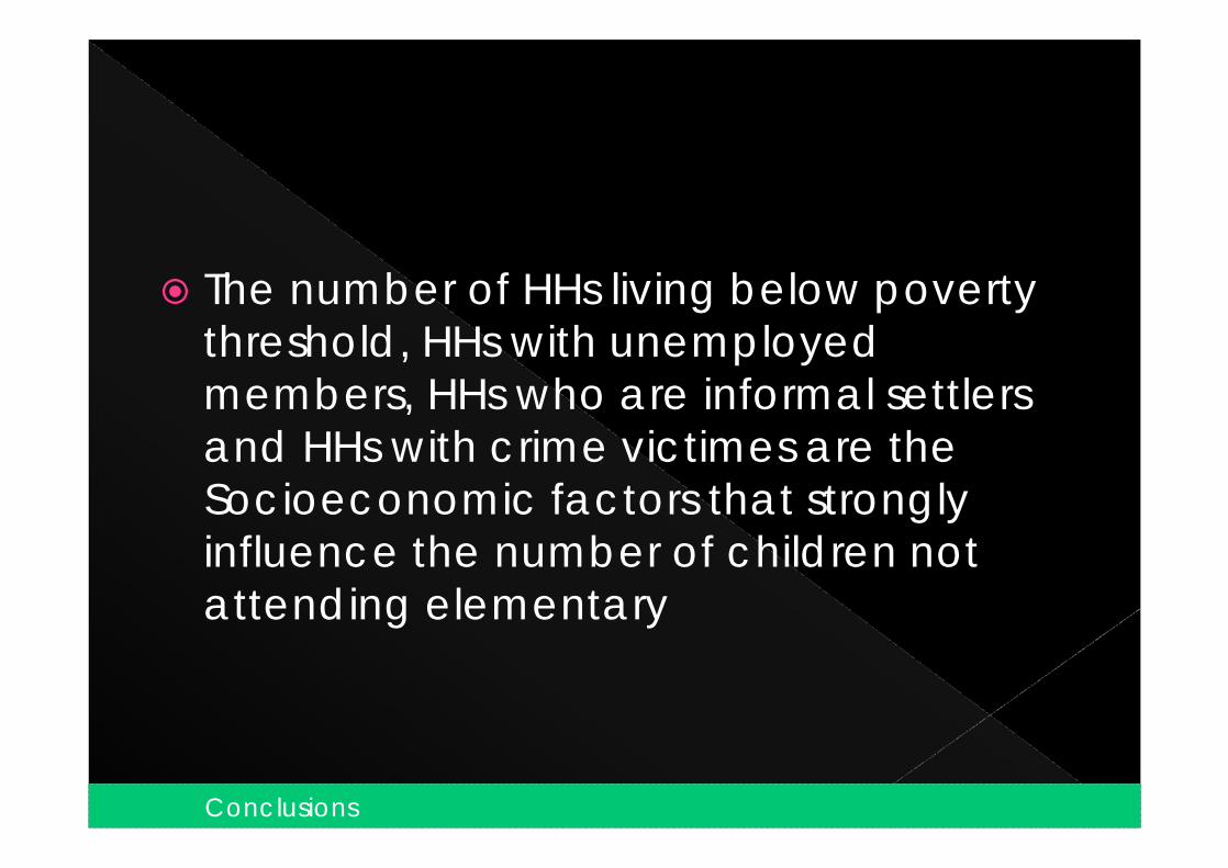
The number of HHs living below poverty threshold, HHs with unemployed members, HHs who are informal settlers and HHs with crime victimes are the Socioeconomic factors that strongly influence the number of children not attending elementary

44Conclusions

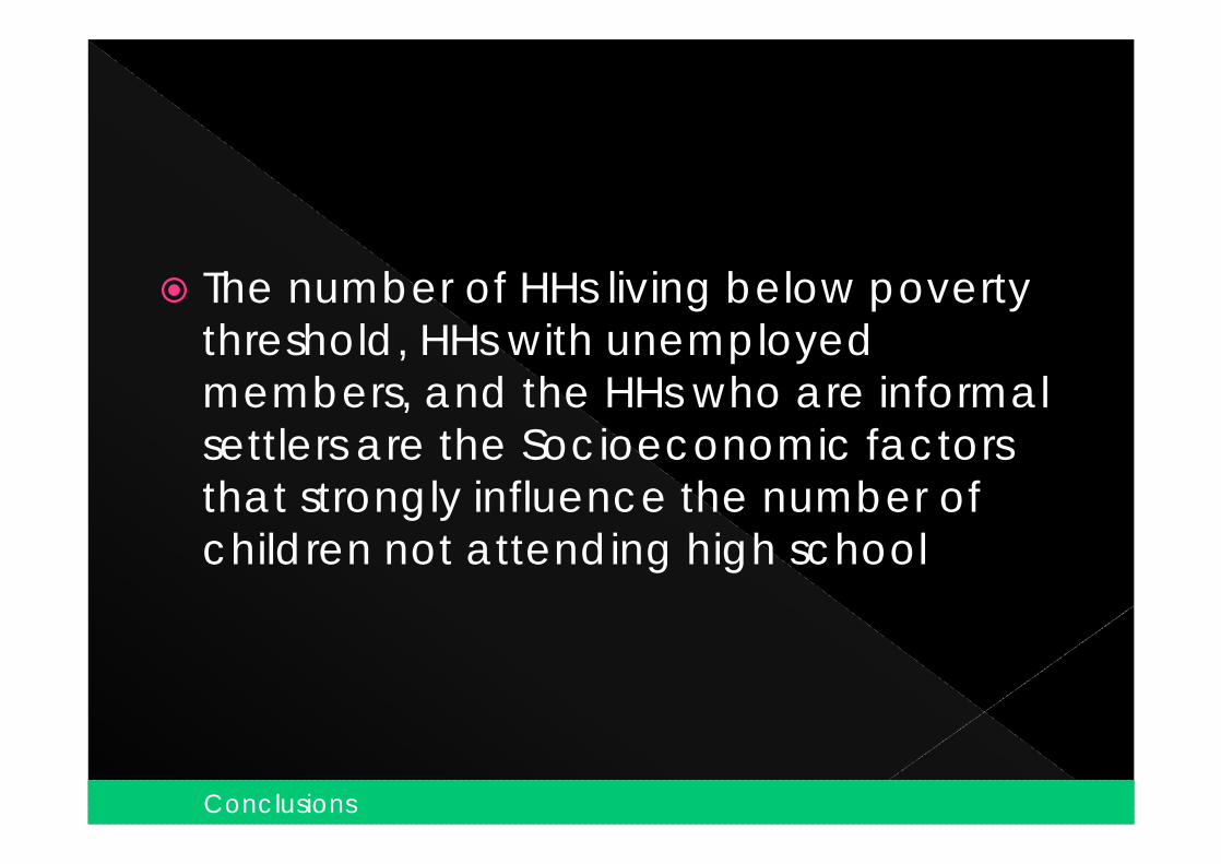
The number of HHs living below poverty threshold, HHs with unemployed members, and the HHs who are informal settlers are the Socioeconomic factors that strongly influence the number of children not attending high school

45Conclusions

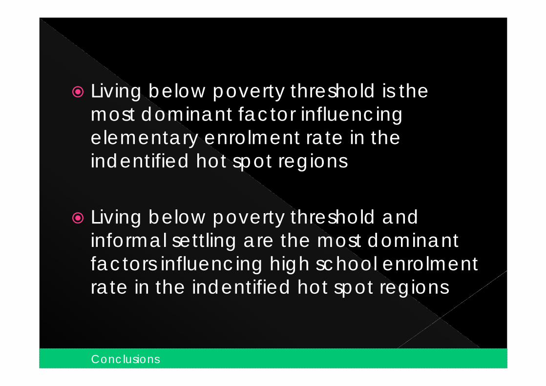
Living below poverty threshold is the most dominant factor influencing elementary enrolment rate in the indentified hot spot regions

Living below poverty threshold and informal settling are the most dominant factors influencing high school enrolment rate in the indentified hot spot regions

46Conclusions

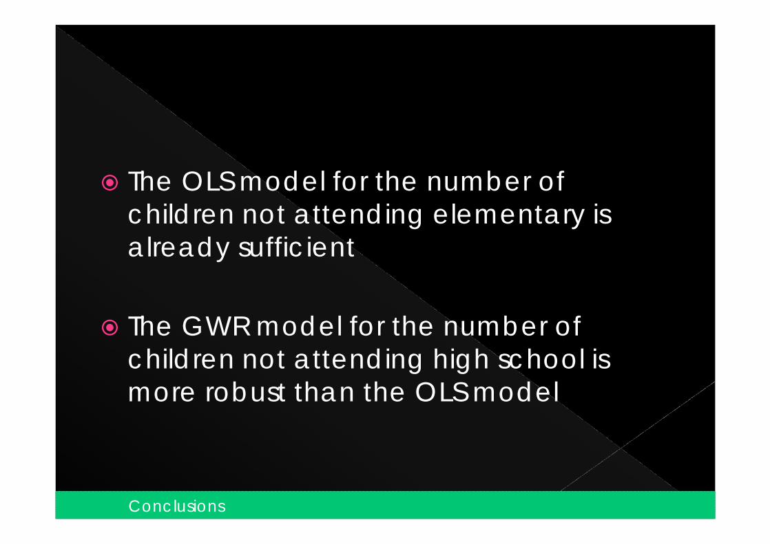
The OLS model for the number of children not attending elementary is already sufficient

The GWR model for the number of children not attending high school is more robust than the OLS model

47Conclusions

Add Spatial Variable to the model (e.g. Distance to Schools)

Investigate the 2005 and 2008 socioeconomic data to check for trends and to further validate the model

48Further Studies

CBMS, 2010. The Many Faces of Poverty in the Province of Batangas, Vol III CBMS. 2008, Monitoring the Achievement of MDG ESRI ® ArcGIS™ 10.0 Help Library Book Bailey and Gatrell. 1995. Interactive Spatial Data Analysis. Pp 168-178,270-278 Brunsdont et al, 1998. Geographically weighted regression – modelling spatial

non-stationarity. The Statistician (1998) 47, Part3, pp. 431-443 Ericta and Fabian. 2009. A documentation of the Philippines’ Family Income

and Expenditure Survey. PIDS Discussion Paper Series No. 2009-18 Maligalig and Albert. 2008. Measures for Assessing Basic Education in the Philippines. PIDS Discussion Paper Series No. 2008-16 Maligalig et. al, 2010. Education Outcomes In the Philippines, ADB Economics

Working Paper Series No. 199 Nava,FJ. 2009. Factors in School Leaving: Variations Across Gender Groups,

School Levels and Locations. Education Quarterly, Vol. 67 (1), 62-78 Orbeta, A.C. 2005. Number of Children and their Education in Philippine

Households. PIDS Discussion Paper Series No. 2005-21

49

The authors would like to thank the following: Dr. Ariel C. Blanco and Prof. Oliver T. Macapinlac Ms. Nieves Borja and the staff of the Tanauan City

Planning and Development Office Engr. Nerio Ronquillo, Engr. Medel Salazar and the

staff of the Provincial Planning and DevelopmentOffice of Batangas

Ms. Celia Reyes, the project leader of the CBMS PEPPhilippines and staff.

50

51

52

Thank you for listening!