ALMA Memo No. 496.1183 GHz water vapour radiometers for ALMA:

Estimation of phase errors under varyingatmospheric conditions.

Alison Stirling, Richard Hills, John Richer, Juan Pardo

July 1, 2004

1 Abstract

We investigate the use of water vapour radiometers as a tool for estimating phase dueto atmospheric water, focusing on the impact of differing atmospheric conditions on therelationship between path length and brightness temperature. We provide a formula forconverting between the two for a variety of atmospheric conditions, and outline how theradiometer channel temperatures may be combined to give an optimal estimate for thepath difference. This estimate gives an error of about 2% per mm of precipitable watervapour due to atmospheric variations. The presence of hydrometeors such as ice or waterdroplets is also considered, and we show that radiometers possessing sideband separationcould be used to detect the presence of 0.02 mm of column integrated ice for crystals ofsize 75µm, and about 10−3 mm of water droplets.

2 Introduction

Astronomical interferometry requires the accurate determination of the path differencebetween light rays received at different antennas. The path difference, however, containsboth information relating to the location of the astronomical source, and contaminationfrom fluctuations in refractive index along the two ray paths. The dominant source offluctuation occurs in the earth’s troposphere, where water vapour and density fluctuationsin the air can affect the path length significantly.

The refractive index, n, of a slab of air can be related to atmospheric water vapour via theSmith-Weintraub equation:

N = 77.6pd

T+ 64.8

pv

T+ 3.776 × 105

pv

T 2, (1)

where N = 106 (Re(n) − 1), T is the temperature in Kelvin, and pd and pv are the partialpressures (in mb) of dry air and water vapour respectively. The first two terms give the

1

contribution to refractivity due to induced dipole transitions, and the third term givesthe refractivity due to the permanent dipole moment of water. The wet refractivity termcontains a small dispersive component due the extended wings of infrared transitions,and requires an adjustment by about 0.5% at 100 GHz, and 2% at 200 GHz. In thisreport, we limit our analysis to the non-dispersive contributions to refractivity, and notethat dispersion in the context of fast switching for ALMA is discussed in more detail inHoldaway & Pardo (2001).

The partial pressures can be expressed in terms of water vapour and dry air densitiesusing the ideal gas equation: pd = ρdRT/Md and pv = ρvRT/Mv where ρd is thedensity of dry air, ρv the water vapour density; R is the universal gas constant (R =8.314 Jmol−1K−1), and Mv = 0.01802 kg mol−1, Md = 0.02896 kg mol−1. This gives

N =(

77.6Rρd

Md

+ 64.8Rρv

Mv

+ 3.776 × 105Rρv

MvT

)

1

100. (2)

In order to calculate the total path delay, L, equation 2 is integrated along the line of sight:

L = 10−6

∫

N (y) dy (3)

where the units of L are the same as the units of y. The path difference between lightreaching two antennas is then given by:

∆L =∫

2.228 × 10−4∆ρT + 0.76 × 10−4∆ρv + 1.742∆(

ρv

T

)

dy, (4)

where ρT is the total air density, and ∆ρ denotes the difference in density along two linesof sight at a given height. Under the hydrostatic approximation, vertical pressure gradi-ents are a function only of the air density, ρT , and so in the absence of horizontal pressurevariations this term is zero to first order. However, this approximation breaks down whenthe atmospheric flow supports vertical accelerations (for example when the flow is turbu-lent), and the variation in ρd will contribute to the phase fluctuations. The effect of thisdry fluctuation term will be considered in another report, and we shall concentrate hereon the impact of water vapour fluctuations on the path. The first of the wet terms is smallcompared with the second, and so the dominant contribution to the phase changes comesfrom the third term, which varies inversely with temperature. We can therefore see fromequation 4 that phase fluctuations depend both on the amount of water vapour presentalong the line of sight, and on the temperature distribution of this water vapour.

The path fluctuations at the ALMA Chajnantor site, measured on a 300 m baseline arein the range 50 − 400µm (Evans et al. ; 2002). Since the aim is to measure the pathper antenna to within {[10 (1 + PWV)]2 +[0.02∆L]2}1/2µm (where PWV is precipitablewater vapour in mm), there is a need to correct for the contribution of the water vapour tothe path. One method is to point the antennas at a known reference source, from whichthe atmospheric phase can be deduced. This fast switching technique is discussed ine.g. Carilli & Holdaway (1999), and Holdaway (2001). A complementary method is tomeasure the amount of water vapour along the line of sight using a radiometer operatingaround the strong water emission line at 183 GHz. The principles of this technique,including the choice of radiometer bands, and the required gain stability are discussed

2

Chan. 1 Chan. 2 Chan. 3 Chan. 4IF/ GHz 0.88 1.94 3.175 5.2

Width/ GHz 0.16 0.75 1.25 2.5

Table 1: Table showing the radiometer bands around the central frequency of 183.31 GHz for theproposed water vapour radiometers.

in Lay (1998); with a model for the phase structure function presented in Carilli, Lay& Sutton (1998). Some preliminary experimental tests have been carried out by e.g.Yun & Wiedner, (1999); Delgado et al. (2001); and Wiedner et al. (2001) who compareinterferometric phases measured on a point-like source with the phase retrieved by theradiometer. These tests show that the relationship between water vapour amount andphase can change depending on the prevailing atmospheric conditions. In this memowe concentrate on quantifying the impact of the atmosphere on phase correction for theradiometers designed for the Chajnantor site.

The prototype Chajnantor radiometers have four channels with IFs and band widths givenin table 1. There are currently two designs, one with a mechanical Dicke switch to look ata reference load, and the other with a cross correlator which looks simultaneously at theload and the atmosphere. The latter has the possibility of being able to separate the upperand lower side-band frequency channels, which may be used to detect the presence of iceand water droplets. This is discussed in section 6.

We have used an atmospheric radiative transfer code (ATM, Pardo, Cernicharo, & Serabyn;2001) to model the radiometric response to phase changes given different water vapourand temperature distributions. In section 3 we look at some basic influences on the 183GHz line profile, and consider the relationship between phase and brightness temperaturein section 4. We also measure the spread in sensitivity values from radiosonde data fromthe Chajnantor site, and in section 5 consider how to combine the estimates of path lengthfrom the different radiometer channels. Section 6 considers the response of the radiomet-ers in the presence of ice and water droplets, and a summary is provided in section 7.

3 The 183 GHz water vapour line – basic influences

In this section we separate out the influences of different atmospheric properties to showtheir effect on the 183 GHz water line. We look at the impact of the water vapour amount;the pressure and temperature of the water vapour; the distribution of temperature withheight; and the distribution of water vapour with height.

3.1 Water vapour amount

We start by looking at how varying amounts of water vapour change the spectrum around183 GHz. The tropospheric temperature profile has been given a constant lapse rate ofΓ = −5.6 K km−1, where

T (z) = Tsurface + Γz, (5)

3

Figure 1: The effect of varying the amount of water vapour in a layer at 1km, with temperature265 K and pressure 500 mb. Solid line is for 0.5 mm of PWV; dot-dashed for 0.675 mm; dashedfor 1.275 mm; dotted, 2.8 mm; and dot-dot-dot-dashed, 6.5 mm.

with surface pressure and temperatures of 560 mb and 270 K. For simplicity the watervapour was placed in a single layer at a height of 1 km and thickness 150 m, and the lineprofile was calculated for 0.5, 0.675, 1.275, 2.8, and 6.5 mm of precipitable water vapour(PWV). These amounts correspond respectively to the 10, 25, 50, 75, and 90 percentilesof the PWV cumulative function at the Chajnantor site (Evans et al. 2002). Figure 1 showsthe line profile for the different water vapour amounts, and shows that the line broadensand the brightness temperature increases with increasing water vapour amount until itsaturates at about 265K.

3.2 Pressure and Temperature

Next we look at how the water vapour line changes with pressure and temperature. Thewater vapour is placed in a single layer, and to alter the pressure without changing thetemperature, we change the height of the layer and set the temperature to be constant withheight (i.e. an isothermal atmosphere). The temperature is changed while keeping thepressure constant by changing the lapse rate, Γ, but keeping the height of the layer con-stant. Figure 2 shows how the line changes with pressure and temperature for 1 mm PWV.The left panel shows that the emission line becomes narrower for lower pressures, withtwo pivot frequencies on either side of the central frequency where the brightness temper-ature is relatively insensitive to pressure. The right panel of figure 2 shows how the line isaffected by the temperature of the water vapour layer. For a 10 K change in temperatureof the layer, the brightness temperature changes by less than 5 K. These experiments showthat the distribution of water vapour with height is important in determining the shape ofthe line profile. We will therefore look at how different water vapour and temperaturedistributions affect the line profile in the next subsection.

4

3.3 Exponential water vapour distributions

To explore the influence of the water vapour distribution on the 183 GHz line profile, wehave created a series of water vapour profiles with an exponential distribution and varyingscale height. Figure 3 shows that the line is narrowest when there is more water at higheraltitudes, where the pressure is lower. This effect diminishes with increasing PWV, whenthe line starts to saturate.

3.4 Varying the lapse rate

Finally we have looked at the brightness temperatures for varying vertical temperaturedistributions, set by the lapse rate, Γ. Typical values for the lapse rate are −5.6 K/kmin moist conditions decreasing to −10 K/km for a very dry atmosphere (this is knownas the dry adiabatic lapse rate). The lapse rate can also be affected by turbulent mixing,and surface cooling, both of which tend to make the lapse rate less negative. For theseexperiments, the water vapour is given an exponential distribution with scale height 2km. Figure 4 shows that the shape of the line profile is relatively insensitive to the tem-perature distribution, and that the maximum value decreases by about 2 K in brightnesstemperature for a 3 K/km increase to the lapse rate.

Figure 2: Bottom panels: Left: The effect of changing the pressure of 1 mm PWV at a fixedtemperature of 265 K. Solid line is for 560 mb; dot-dashed for 480 mb; dashed 415 mb; anddotted, 375 mb. Right: The effect of changing the temperature of 1 mm PWV at a fixed pressureof 491 mb. Solid line is for 264.2 K; dot-dashed for 260.1 K; dashed, 256.1 K; and dotted, 252.2K. Top panels show the difference in T BRI of each line compared with the solid line.

5

Figure 3: The effect of changing the scale height, h0, on the brightness temperature. Top leftfor PWV = 0.5; top right PWV = 0.675; bottom left PWV = 1.275; bottom right PWV = 2.8(representing the 10, 25, 50 and 75 percentile frequency values). h0 takes the values 0.5,1.0,1.5,2.0km corresponding to solid, dot-dashed,dashed and dotted lines respectively. The top plots of eachpanel show the difference in brightness temperature of each line compared with the solid line.

6

Figure 4: The effect of changing the lapse rate, Γ, on brightness temperature. Top left for PWV =0.5; top right PWV = 0.675; bottom left PWV = 1.275; bottom right PWV = 2.8 mm (representingthe 10,25,50 and 75 percentile frequency values). Γ takes values −2.5,−5,−7.5,−10.0 K/kmcorresponding to solid, dot-dashed,dashed and dotted lines respectively. The top plots of eachpanel show the difference in brightness temperature of each line compared with the solid line.

7

4 Radiometric sensitivity to phase for different atmosphericconditions

4.1 Introduction

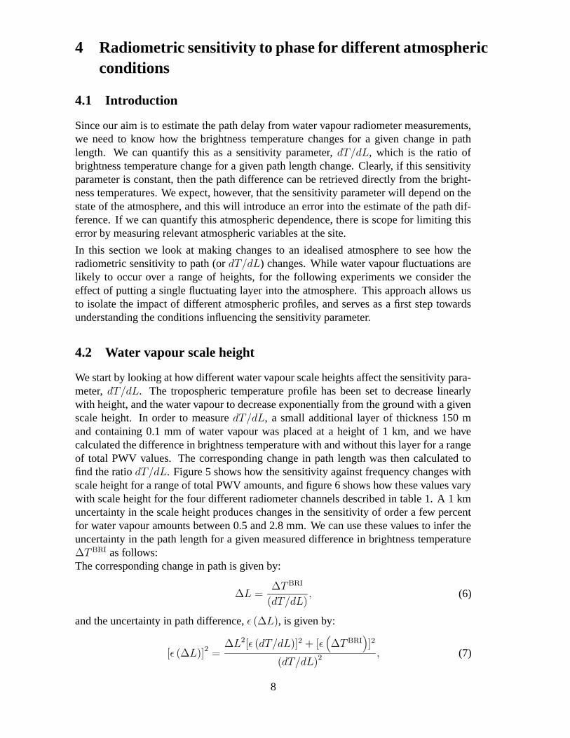
Since our aim is to estimate the path delay from water vapour radiometer measurements,we need to know how the brightness temperature changes for a given change in pathlength. We can quantify this as a sensitivity parameter, dT/dL, which is the ratio ofbrightness temperature change for a given path length change. Clearly, if this sensitivityparameter is constant, then the path difference can be retrieved directly from the bright-ness temperatures. We expect, however, that the sensitivity parameter will depend on thestate of the atmosphere, and this will introduce an error into the estimate of the path dif-ference. If we can quantify this atmospheric dependence, there is scope for limiting thiserror by measuring relevant atmospheric variables at the site.

In this section we look at making changes to an idealised atmosphere to see how theradiometric sensitivity to path (or dT/dL) changes. While water vapour fluctuations arelikely to occur over a range of heights, for the following experiments we consider theeffect of putting a single fluctuating layer into the atmosphere. This approach allows usto isolate the impact of different atmospheric profiles, and serves as a first step towardsunderstanding the conditions influencing the sensitivity parameter.

4.2 Water vapour scale height

We start by looking at how different water vapour scale heights affect the sensitivity para-meter, dT/dL. The tropospheric temperature profile has been set to decrease linearlywith height, and the water vapour to decrease exponentially from the ground with a givenscale height. In order to measure dT/dL, a small additional layer of thickness 150 mand containing 0.1 mm of water vapour was placed at a height of 1 km, and we havecalculated the difference in brightness temperature with and without this layer for a rangeof total PWV values. The corresponding change in path length was then calculated tofind the ratio dT/dL. Figure 5 shows how the sensitivity against frequency changes withscale height for a range of total PWV amounts, and figure 6 shows how these values varywith scale height for the four different radiometer channels described in table 1. A 1 kmuncertainty in the scale height produces changes in the sensitivity of order a few percentfor water vapour amounts between 0.5 and 2.8 mm. We can use these values to infer theuncertainty in the path length for a given measured difference in brightness temperature∆TBRI as follows:The corresponding change in path is given by:

∆L =∆TBRI

(dT/dL), (6)

and the uncertainty in path difference, ε (∆L), is given by:

[ε (∆L)]2 =∆L2[ε (dT/dL)]2 + [ε

(

∆TBRI)

]2

(dT/dL)2, (7)

8

so for large path differences the sensitivity parameter is the dominant contribution tothe uncertainty in the path difference and for small ∆L the uncertainty in the sensitivityparameter becomes small, and the errors due to noise in the radiometer dominate.

4.3 Height of the fluctuating layer

Next we change the height of the additional water vapour layer, z0, and use an exponentialprofile of water vapour with fixed scale height of 1 km. The height of the fluctuatinglayer is expected to affect the sensitivity for two reasons. Firstly the change in brightnesstemperature when the layer is higher will be narrower with frequency due to the lowerpressure of this layer, and secondly the higher the layer the lower its temperature, andso the greater the path delay contribution. dT/dL is therefore expected to be lower inamplitude for higher layers, but vary more sharply with frequency around 183.31GHz.Figures 7 and 8 show the resulting sensitivities, with a 1 km uncertainty in the heightof the fluctuating layer giving sensitivity changes of between 4 − 10% for water vapouramounts between 0.5 and 2.8 mm.

4.4 Lapse rate

In a third numerical experiment the vertical tropospheric temperature distribution wasaltered by changing the lapse rate, while the water vapour scale height was fixed at 2 km,and the height of the fluctuating layer was placed at 2 km. Figures 9 and 10 show how thesensitivity varies with temperature distribution for linear tropospheric temperature profilesranging between −2.5 K km−1 down to −10 K km−1.

For a 1 K km−1 uncertainty in the lapse rate, the sensitivity changes typically by lessthan 1 % for PWV values between 0.5 and 2.8 mm. Since the brightness temperaturesare relatively insensitive to the temperature of the fluctuating layer, but the path delayis proportional to T−1, we can convert these results into a dependence of dT/dL on thetemperature of the fluctuating layer. For this we find that the uncertainty in the path lengthis again of order 1 % per Kelvin for 0.5 − 2.8 mm PWV.

9

Figure 5: The effect of changing the scale height, h0, on the brightness temperature. Top leftfor PWV = 0.5; top right PWV = 0.675; bottom left PWV = 1.275; bottom right PWV = 2.8 mm(representing the 10, 25, 50 and 75 % frequency values). h0 takes the values 0.5,1.0,1.5,2.0 kmcorresponding to solid, dot-dashed, dashed and dotted lines respectively. The top plots of eachpanel show the difference in brightness temperature of each line compared with the solid line.

10

Figure 6: The effect of changing the scale height, h0, on the radiometer channel sensitivity,dT/dL. Top left for PWV = 0.5; top right PWV = 0.675; bottom left PWV = 1.275; bottom rightPWV = 2.8 mm (representing the 10,25,50 and 75 % frequency values).Crosses correspond tochannel 1, squares to channel 2, triangles to channel 3 and circles to channel 4.

11

Figure 7: The effect of changing the height of the fluctuating layer, z 0 on the sensitivity parameter,dT/dL. Top left for PWV = 0.5; top right PWV = 0.675; bottom left PWV = 1.275; bottom rightPWV = 2.8 mm (representing the 10, 25, 50 and 75 % frequency values). z0 takes the values 0.5,1.0, 1.5, 2.0 km above ground level, corresponding to solid, dot-dashed,dashed and dotted linesrespectively. The top plots of each panel show the difference in dT/dL of each line comparedwith the solid line.

12

Figure 8: The effect of changing the height of the fluctuating layer, z 0 on the radiometer channelsensitivity, dT/dL. Top left for PWV = 0.5; top right PWV = 0.675; bottom left PWV = 1.275;bottom right PWV = 2.8 mm (representing the 10, 25, 50 and 75 % frequency values). Crossescorrespond to channel 1, squares to channel 2, triangles to channel 3 and circles to channel 4.

13

Figure 9: The effect of changing the lapse rate, Γ, on the sensitivity dT/dL. Top left for PWV =0.5; top right PWV = 0.675; bottom left PWV = 1.275; bottom right PWV = 2.8 mm (representingthe 10,25,50 and 75 % frequency values). Γ takes values -2.5, -5, -7.5, -10. K/km correspondingto solid, dot-dashed,dashed and dotted lines respectively.

14

Figure 10: The effect of changing the lapse rate, Γ, on the radiometer channel sensitivity, dT/dL.Top left for PWV = 0.5; top right PWV = 0.675; bottom left PWV = 1.275; bottom right PWV =2.8 mm (representing the 10,25,50 and 75 % ile frequency values). Crosses correspond to channel1, squares to channel 2, triangles to channel 3 and circles to channel 4.

15

4.5 Combining results

Since the sensitivity parameter dT/dL appears to have a linear dependence on z0, h0 andΓ0, we can combine the results from the previous sections to produce a linear fitted for-mula for dT/dL as a function of z0, h0 and Γ0 for the different channels and for differentamounts of PWV. This will enable us to estimate the uncertainty in dT/dL depending onthe constraints we can provide for z0, h0 and Γ0. Assuming dT/dL can be parametrisedwith a linear fit in each of the three directions z0, h0 and Γ0, we can write dT/dL as:

dT

dL= axyz + bxy + cxz + dyz + ex + fy + gz + h, (8)

where a − h are constants, and

x =h0 − hmin

0

hmax0 − hmin

0

; y =Γ0 − Γmin

0

Γmax0 − Γmin

0

; z =z0 − zmin

0

zmax0 − zmin

0

(9)

and

hmin

0= 0.5 km; Γmin

0= −10.0 K km−1; zmin

0= 0.5 km

hmax

0= 2.0 km; Γmax

0= −2.5 K km−1; zmax

0= 2.0 km. (10)

The coefficients a − h can be found by calculating the sensitivity parameter for a cubeof 8 (x, y, z) values, each taking values 0 and 1, and where x, y, z are defined in equa-tion 9. The coefficients have been calculated for each of the channels and a range of PWVamounts, and the values are summarised in table 2.

We can also express the uncertainty in the sensitivity parameter in terms of the uncertaintyin the values of the scale height, lapse rate, and height of the fluctuating layer. Assumingthat these quantities vary independently, the uncertainty can be expressed as:

[

ε

(

dT

dL

)]2

= [ε (x)]2(

∂ dTdL

∂x

)2

y,z

+ [ε (y)]2(

∂ dTdL

∂y

)2

x,z

+ [ε (z)]2(

∂ dTdL

∂z

)2

x,y

= [ε (x)]2 (ayz + by + cz + e)2 +

[ε (y)]2 (axz + bx + dz + f)2 +

[ε (z)]2 (axy + cx + dy + g)2 . (11)

We can now estimate the total expected uncertainty in dT/dL for each channel. Firstly wehave estimated the uncertainty in lapse rate and scale height from 200 radiosonde ascents(Radford et al. , 2003) taken over a period of four years at Chajnantor. This gave valuesfor the scale height and lapse rate of Γ0 = −6.8 ± 1.5 K km−1, and h0 = 1.5 ± 1.0km. For the height of the fluctuating layer, we have used a value from Robson et al.(2000), who found z0 = 0.4 ± 0.3 km during their observing run. Table 3 shows theexpected sensitivity values, and their associated uncertainty, which is generally in therange 2 − 5%. It is worth noting at this stage that these values assume that the PWV iswell known. Clearly an uncertainty in the PWV will increase the uncertainty in dT/dL,and this will be considered in more detail in a later report.

Since the parametrisation for dT/dL in equation 8 makes the assumption that the wa-ter vapour is exponentially distributed and that the temperature decreases linearly with

16

PWV /mm Channel a b c d e f g h

0.50 1 0.69 0.37 -1.16 1.14 -1.88 0.59 1.50 26.590.50 2 0.21 0.36 -0.27 0.17 0.07 0.28 -1.23 20.590.50 3 0.05 0.14 -0.07 -0.06 0.16 0.10 -1.63 13.650.50 4 0.01 0.04 -0.00 -0.07 0.06 0.02 -1.16 7.330.68 1 0.77 0.27 -1.28 0.96 -1.83 0.54 1.14 20.840.68 2 0.26 0.41 -0.34 0.16 0.11 0.30 -1.10 17.920.68 3 0.07 0.18 -0.09 -0.05 0.20 0.11 -1.53 12.640.68 4 0.01 0.05 -0.00 -0.07 0.07 0.02 -1.13 7.061.27 1 0.79 -0.18 -1.27 0.52 -1.01 0.34 0.44 9.091.27 2 0.36 0.40 -0.47 0.14 0.24 0.31 -0.76 11.171.27 3 0.11 0.25 -0.14 -0.03 0.32 0.16 -1.24 9.711.27 4 0.02 0.08 -0.01 -0.06 0.12 0.04 -1.03 6.222.80 1 0.47 -0.43 -0.69 0.11 0.23 0.06 0.02 1.152.80 2 0.38 0.10 -0.51 0.07 0.42 0.18 -0.30 3.412.80 3 0.17 0.24 -0.23 -0.01 0.47 0.17 -0.72 5.002.80 4 0.04 0.12 -0.03 -0.04 0.22 0.07 -0.83 4.54

Table 2: Table showing the parameters required to obtain dT/dL as a function of scale height,fluctuating layer height, and lapse rate. Parameters a, b, c, d, e, f, g, h are defined in equations 8and 9, and have units K mm−1.

PWV/ mm Chan. 1/ K mm−1 Chan. 2 / K mm−1 Chan. 3 / K mm−1 Chan. 4/ K mm−1

0.50 25.58 +/- 1.20 20.95 +/- 0.31 13.95 +/- 0.37 7.47 +/- 0.240.68 19.85 +/- 1.17 18.32 +/- 0.32 12.98 +/- 0.37 7.21 +/- 0.241.27 8.50 +/- 0.72 11.65 +/- 0.36 10.16 +/- 0.40 6.41 +/- 0.242.80 1.23 +/- 0.08 3.83 +/- 0.36 5.52 +/- 0.44 4.81 +/- 0.25

Table 3: Table showing the expected values and uncertainties of dT/dL for typical uncertaintiesin Γ0, h0 and z0. (Γ0 = −6.8 ± 1.5 K km−1, h0 = 1.5 ± 1.0 km, and z0 = 0.4 ± 0.3km).

height, it is worth comparing our prediction with dT/dL measured from real atmosphericdata from the Chajnantor site. Again we use the 200 radiosonde data profiles to providerealistic water vapour and temperature profiles. The locations of the fluctuating layers ofwater vapour are not readily obtained from single radiosonde ascents, so for comparisonwe have used the same approach as the earlier experiments, and inserted an additionalwater vapour layer of 0.1 mm at 1 km and thickness 150 m to represent the fluctuatinglayer, and calculated the brightness temperature change due to this layer, along with theassociated change in path length. Since z0 has been held constant for the above analysis,we set ε (z) = 0 for this comparison. Figure 11 shows the predicted dT/dL values withassociated errors from equations 8 and 11, with the values found for the radiosonde as-cents overlaid. There is good agreement between our parametrised fit and the radiosondedata, suggesting that the use of a linear fit to dT/dL, and the assumptions of exponentialwater vapour profiles with constant lapse rates are reasonable approximations to make.

Clearly it is desirable to minimise our uncertainty in the values of Γ0, h0, and z0, and thismay to a large part be achieved by using a separate instrument to measure the temperatureprofile. While the temperature profile will give a much better estimate for Γ0, it may also

17

0 1 2 3 4PWV /mm

0

10

20

30

40

50

dT/d

L /

K/m

m

0 1 2 3 4PWV /mm

0

5

10

15

20

25

30

dT/d

L /

K/m

m

0 1 2 3 4PWV /mm

0

5

10

15

20

dT/d

L /

K/m

m

0 1 2 3 4PWV /mm

0

2

4

6

8

10

dT/d

L /

K/m

m

Figure 11: Comparison of dT/dL measured from radiosonde ascents with associated predictions.Each point represents dT/dL calculated from a radiosonde profile, and error bars show the pre-dictions from equations 8 and 11. Top left is for channel 1, top right for channel 2, bottom left forchannel 3, bottom right for channel 4.

18

provide information relating to h0 and z0. One example of where h0 and z0 may be linkedto the temperature profile is in the presence of a temperature inversion. This tends toprevent air from below mixing with air from above the inversion, and so the transport ofwater vapour upwards is also curtailed. The extent of the water vapour distribution thentends to be set by the height of the inversion. In cases where the water vapour profileexperiences a sharp cut off at a given height, very slight vertical mixing can give rise toa high difference in water vapour amount at that height, and so the fluctuating layer ofwater vapour is most likely also to be set by the height of the inversion. We are currentlyinvestigating how often, and how reliably one can obtain information about the watervapour profile from the temperature profile.

One instrument that would be able to measure the temperature profile is a seven-channelradiometer that measures emission from oxygen lines between 51–59 GHz. Typicallythese oxygen radiometers can measure temperature profiles with an r.m.s. error of lessthan 1 K up to 1 km above ground level, increasing to 1.5 K at 6 km. There is some un-certainty about the vertical resolution of such an instrument, and in particular it may notresolve higher level temperature inversions, which could increase the uncertainty in tem-perature to about 3 K at an inversion. The dominant water vapour fluctuations, however,are expected to be concentrated at lower levels where inversions are better represented. Inthis case, the instrument could allow us to reduce the uncertainty in path due to temperat-ure to about 1%.

5 Combining path estimates from the different channels

Now that we have modelled the relationship between brightness temperature and pathlength, we can take an initial look at the question of how best to combine the values beingproduced by the four channels of the radiometer. In general this will be done by takingthe temperature from each channel, subtracting from it some reference value, so we havethe fluctuation in the temperature, and then dividing by the sensitivity parameter (dT/dL)to get the corresponding path fluctuation. (The reference value might be the averagetemperature for that channel over all the radiometers on the array, or a value taken fromthe most recent observation of a calibrator.) We will then have four estimates of the pathfluctuation. If there were no noise on the data and our model were perfect, these shouldbe identical. Since there will be both noise in the data and uncertainty in the model, theywill not agree and we need to find the best way of combining them. The simplest thing todo is to form a weighted average of the four values of the path fluctuation.

In the case where the fluctuations are small, our main concern is to minimise the errorsintroduced by the noise and residual gain fluctuations in the radiometer. The procedurein this case is straight-forward: we estimate the errors expected in the individual chan-nels and convert these into errors in the path. Assuming these errors to be independent,which should be true so long as noise dominates, we can then use the standard result thatthe weights should be inversely proportional to the squares of the errors. Table 5 givesexamples of this. For details of the noise estimates see Hills (2004).

As the fluctuations become larger we become less concerned about the noise and moreconcerned about the accuracy of the conversion, as discussed in the previous section. As

19

PWV / mm Channel 1 /µm Channel 2 /µm Channel 3 /µm Channel 4 /µm0.5 10.9 6.7 9.6 17.70.68 14.1 7.3 9.6 17.41.27 34.1 11.3 10.3 16.32.8 247.8 41.3 19.7 15.4

Table 4: Expected errors in retrieved path due to noise for each radiometer channel for a range ofPWV values. (εBi

/{dT/dL})

an extreme case we could choose a set a weights such that the average is independent ofthese various parameters. Another approach is to incorporate the uncertainty in dT/dLinto the path error estimate having weighted the channels with one over the radiometernoise squared. We outline this method below.

Let Bi = ∆TBRIi i.e. the measured brightness temperature change in channel i, with an

error due to radiometer noise, εBi(see table 4). For ease of notation we call the sensitivity

parameter for channel i Si ≡ dT/dL, which is a function of the atmospheric variablesx, y, z (defined in equation 9) which are allowed to vary independently. The sensitiv-ity parameter has errors associated with the uncertainties in the atmospheric parametersx, y, z, and we call these εSx

i, εSy

i, εSz

irespectively.

The path difference, ∆Li, as measured in channel i is then given by

∆Li = Bi/Si. (12)

We first construct weights for finding an optimal estimate for the path from the four chan-nels assuming there is no error in Si:

∆L =∑

i

wiBi

Si

, (13)

where

wi =S2

i

εBi2; and wi =

wi∑

i wi

. (14)

The error in path due to the radiometer noise is given by:

(ε∆Lnoise)2 =

∑

i

w2i εBi

2

S2i

=1

∑

i wi

, (15)

and some examples for this are shown in table 5.

We can add in the contribution to path error from uncertainties in dT/dL as follows:First consider the error introduced into ∆L by an uncertainty in the parameter x. So nowx → x ± ∆x, and εSx

i= Si (x + ∆x) − Si (x). So now the error in the path difference

due to uncertainty in x is:

ε∆Lx=∑

i

wiBi

Si (∆x + x)−

wiBi

Si (x)'∑

i

wiBiεSxi

S2i

. (16)

20

PWV w1 w2 w3 w4 ε∆Lnoiseε∆Lx,y,z

ε∆LTotal

/mm /µm /µm /µm0.5 0.188 0.496 0.245 0.071 4.7 5.2 7.00.68 0.132 0.494 0.287 0.087 5.1 6.4 8.21.27 0.039 0.359 0.359 0.171 6.7 12.5 14.22.8 0.002 0.080 0.348 0.570 11.6 25.2 27.70.5 0.233 0.607 0.153 0.007 5.0 4.3 6.60.68 0.212 0.602 0.177 0.009 5.6 4.9 7.41.27 0.180 0.451 0.451 0.095 8.6 7.8 11.62.8 0.003 -0.019 0.091 0.924 14.4 21.5 25.8

Table 5: The channel weights required to minimise the path error due to noise (wi) and associatedestimate for this path error, ε∆Lnoise

; an estimate of the error due to uncertainty in the conversionfactor, ε∆Lx,y,z

; and estimate for the total combined path error ε∆LTotal. These values have been

obtained assuming a total path difference, ∆L, of 400 µm. Top half of table uses weights fromequation 14, bottom half of table shows how these estimates change when the weights are reoptim-ised to minimise the total path error.

The total error in the path difference due to uncertainties in x, y, and z can be found byadding ε∆Lx,y,orz

in quadrature:

(

ε∆Lx,y,z

)2

= (ε∆Lx)2 +

(

ε∆Ly

)2

+ (ε∆Lz)2 . (17)

The total error in path is then found by combining the error due to radiometer noise andthe error due to uncertainties in x, y, z:

(ε∆LTotal)2 = (ε∆Lnoise

)2 +(

ε∆Lx,y,z

)2

. (18)

Finally, since the weights wi were chosen to minimise the error in the noise alone, wecan adjust these using a suitable optimisation procedure to give weights that minimise thetotal error. This approach is illustrated in table 5, which gives the final error estimate withand without the adjusted weights. It can be seen that the modification in weights onlyreduces the path error by a few percent. Figure 12 shows how the path error is expected tochange with PWV for the values in table 5, with this method enabling a retrieval of pathdifference with an error of given by:

ε∆LTotal={

[3.7 (1 + PWV)]2 + [0.02∆LPWV]2}

1

2 µm (19)

where the first term is due to radiometer noise, and the second is due to uncertainties inatmospheric parameters. While this is an encouraging result, it should be noted that thereare number of additional sources of error to consider, for example uncertainty in PWV;water vapour fluctuations distributed over a range of heights; and radiometer calibrationerrors. Future work will concentrate on broadening this analysis to take account of themore general case.

21

0 1 2 3PWV /mm

0

10

20

30

40

50

Path

err

or /

mic

rons

Figure 12: The predicted uncertainty in path length for a total path length of 400µm. Starstake account only of radiometer noise (equation 15) and triangles include the dT/dL uncertainties(equation 18), with adjustments to the weights to minimise this error (table 5). The solid lineshows the error specification (given by {[10 (1 + PWV)]2 + [0.02∆L]2}1/2µm).

6 The effect of hydrometeors on the path measurements

6.1 Ice

In this section we look at the expected performance of the WVR’s in the presence of iceand liquid water hydrometeors in the atmosphere. While ice is not expected to affect theatmospheric refractive index significantly, if it contributes to the radiometric brightnesstemperature, it is likely to change the sensitivity parameter, dT/dL. It is therefore worthexploring how ice affects the brightness temperatures, and whether its presence can bedetected by the WVR’s. We have used the ATM to calculate brightness temperatures inthe presence of ice particles (and in the next section water droplets), and details of theATM modelling of hydrometeors can be found in Wiedner et al. (2004).

Ice scattering depends on the shape and alignment of the ice crystals as well as their size.For this work, we have assumed that the dominant source of ice crystals at the Chajnantorsite is through orographic lifting of supersaturated air. This tends to generate spherical iceparticles, since they are formed by freezing existing water droplets, with little subsequentaccretion, and typically they have sizes around 75 µm (e.g. Scorer, 1997). Ice crystalsformed as part of a cloud system tend to be larger, with typical sizes of 250 µm anda density of about 0.025 g m−3 over a 1.5 km layer (Dowling & Radke; 1990), (thiscorresponds to about 0.04 mm of column integrated water).

We first perform an experiment in which a layer of ice is incorporated between 1 and 2.5

22

km above the Chajnantor site, with ice water amount ranging between 0.05 and 0.15 mm,and radii of 100 and 200 µm. Figure 13 shows how the brightness temperature around the183 GHz water line is changed by the presence of the ice. While 0.15 mm of crystals ofradius 100 µm change the brightness temperature by about 2 K, at 200 µm the increaseis closer to 12 K, showing that there is high sensitivity to particle size. The effect of theice is two-fold – the first is to reduce the difference in brightness temperature between thewings of the water line profile and the maximum, and the second is to introduce additionalasymmetry into the shape of the profile. While the first of these features is detectable witha double sideband radiometer, the second would only be detectable if the upper and lowersidebands can be separated, as is possible with a cross correlator radiometer.

The first effect can be detected by looking at the difference between pairs of radiometerchannels (i.e. 1-4;2-4;3-4;2-3;1-3;1-2) and subtracting off the expected differences in theabsence of ice. The asymmetry can be found by looking at the difference in brightnesstemperature between the upper and lower sidebands and again subtracting off the asym-metry in the absence of ice. Figure 14 shows these quantities for 100 and 200 µm spher-ical ice crystals. While the cross channel values of ∆T BRI gives a larger signal, there isgreater scope for confusion of this signal with other atmospheric conditions, for examplewater vapour distributions with a small scale height, which also act to reduce the heightdifference between the maximum and the wings of the profile.

In order to investigate whether sideband separation would be a useful property for theChajnantor water vapour radiometers, it is worth calculating how much ice (and of whatsize) would have to be present in order for it to be detectable by the radiometer. Wehave used the radiometer equation to estimate the likely noise on brightness temperatureestimates, which gives a limit to the sensitivity of the radiometer to the presence of asym-metry. We have then calculated the expected asymmetry for a grid of ice amounts andsizes, and plotted contours delineating levels of asymmetry that would be expected to bedetectable at the 1,2 and 3 σ level. Figure 15 shows that the sensitivity to ice is greatestwhen crystals have radius ∼ 250µm, which is about λ/2π at the radiometer frequencies.This is what we might expect, since Mie theory predicts that the extinction cross sectionfor spheres is at a maximum when the ratio of the particle circumference to the incidentlight wavelength is around unity. At 75 µm the sideband-separating radiometer would becapable of detecting ice amounts greater than 0.04 mm to 1σ and about 0.1 mm to 2σ inchannel 4.

23

Figure 13: The impact of varying amounts of ice on brightness temperatures. The ice particlesare spherical with radius 100 in the top panels, and 200 µm in the bottom panels. Left panels showthe brightness temperature, and right panels show the change in brightness temperature as a resultof the ice (solid line is for no ice; dot-dashed for 0.05 mm of ice; dashed for 0.1 mm; and dottedfor 0.15 mm).

24

Figure 14: Top panels show the additional asymmetry between the upper and lower sidebandchannels compared with the no-ice case (crosses for channel 1, squares for channel 2, triangles forchannel 3 and circles for channel 4). (left is for 100 µm, and right for 200 µm). Bottom panelsshow a measure of the difference in brightness between the different channels (see text). (crosses:1-4, squares 1-3, triangles 1-2, circles with + 2-4, dotted circles 2-3, open circles 3-4).

25

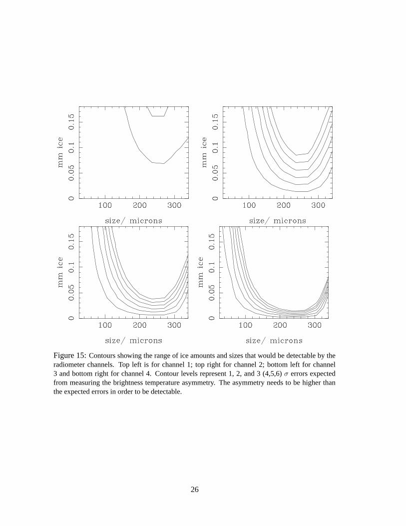
Figure 15: Contours showing the range of ice amounts and sizes that would be detectable by theradiometer channels. Top left is for channel 1; top right for channel 2; bottom left for channel3 and bottom right for channel 4. Contour levels represent 1, 2, and 3 (4,5,6) σ errors expectedfrom measuring the brightness temperature asymmetry. The asymmetry needs to be higher thanthe expected errors in order to be detectable.

26

6.2 Water droplets

Water droplets are also expected to produce an asymmetry in the 183 GHz line profile, andso we can apply the same approach to calculate the expected sensitivity to the presenceof the droplets. Again, we assume that a likely source of water droplets is from loweraltitude air being forced up onto the plateau, where it is cooled and the water vapourcondenses to form fog. Water droplets in fog typically have sizes of 5 − 30µm, andconcentrations of order 10 droplets per cm3 (e.g. Kunkel, 1971). We place the fog in alayer between 1 and 2.5 km above the ground for this study. Figure 16 shows how thebrightness temperature changes with increasing number density of droplets each of size 10µm, and how the brightness temperature changes with size of droplets for a given amountof liquid water. Again the effect is to reduce the difference in brightness temperaturebetween the maximum and the wings, and to introduce an asymmetry into the profile.

Figure 17 shows the asymmetry between the upper and lower sideband brightness tem-peratures for different liquid water amounts and droplet sizes. The asymmetry increaseswith water droplet concentration, but is relatively insensitive to droplet size. Again wecan calculate how much liquid water would need to be present in order to be detectableby the radiometer, and figure 18 shows that the radiometer would be sensitive to amountsgreater than 0.002 mm (which would correspond to a droplet concentration of just under1 droplet per cm3).

27

Figure 16: The impact of varying amounts of liquid water on brightness temperatures. Top panelsshow the effect of varying amounts of liquid water of droplet size 10µm (solid line is for no liquidwater; dot-dashed for 0.05 mm of droplets; dashed for 0.1 mm; and dotted for 0.15 mm), andbottom panels show the effect of varying the radius of the water droplets for an amount of 0.1 mm(solid is for 50 µm; dot-dashed for 100; dashed for 200; and dotted for 300 µm, and dot-dot-dot-dashed is for no hydrometeor). Left panels show the brightness temperature, right panels show thechange in brightness temperature as a result of the droplets.

28

Figure 17: Left panel shows the additional asymmetry resulting from varying concentrations ofwater droplets of size 10 µm. Right panel shows the asymmetry for varying sizes of water dropletand 0.1 mm of liquid water. Crosses are for channel 1, squares for channel 2, triangles for channel3 and circles for channel 4.

Figure 18: Contours showing the amount of liquid water expected to be detectable from a meas-urement of the asymmetry of the line profile. Top left is for channel 1 (nothing detectable in thischannel) ; top right for channel 2; bottom left for channel 3; bottom right for channel 4.

29

7 Summary

In this report we have investigated the effect of changing atmospheric conditions on theradiometric sensitivity to path fluctuations. We have performed idealised experiments tomodel how quantities such as the water vapour scale height, the temperature profile, andthe height of fluctuating water vapour influence the sensitivity. We have also measuredthe range of these properties from radiosonde data, and inferred a value for the uncertaintyin the conversion factor between brightness temperature and path length of about 4% forPWV amounts of 1.275 mm or less. We have suggested how the four radiometer channelsmight be combined optimally to produce a best estimate for the path length, and find usingthis method a fractional path length error due to the atmosphere of about 2PWV%.

We have also investigated the influence of hydrometeors on the line profiles, focusing onthe extent to which sideband separation might be used to detect the presence of ice orwater droplets. We find that the Chajnantor radiometers could be sensitive to ice amountsover 0.02 mm, and water droplet amounts over 10−3 mm if sideband separation is per-formed.

Future work on the wet fluctuations will concentrate on extending the error analysis tothe case where PWV is not known exactly, and where vapour fluctuations are no longerconfined to a single layer. The amplitude of dry fluctuations under varying atmosphericconditions should also be considered. Since there is scope for improving path variationestimates with additional calibration devices at the site such as a temperature profiler, itwill also be worth evaluating how much these can be expected to assist our estimates ofthe path length.

8 References

Carilli, C.L. & Holdaway, M.A., 1999, ALMA memo 262, ‘Tropospheric Phase Calibra-tion in Millimeter Interferometry’

Carilli, C.L., Lay, O.P., & Sutton, E.C., 1998, ALMA memo 210, ‘Radiometric phasecorrection’

Delgado, G., Otarola, Nyman, L-A. et al. 2000, ALMA memo 332, ‘Phase correction ofinterferometer data at Mauna Kea and Chajnantor’

Delgado, G., 2001, ALMA memo 361, ‘Phase Cross-Correction of a 11.2 GHz Interfero-meter and 183 GHz Water Line Radiometers at Chajnantor’

Dowling, D.R., Radke, L.,1990, Journal of Applied Meteorology, Vol 29, 970, ‘A sum-mary of the physical properties of cirrus clouds’

Evans, N., Richer, J., Sakamoto, S., Wilson, C., Mardones, D., Radford, S., Cull, S.,Lucas, R., 2003, ALMA memo No. 471, ‘Site Properties and Stringency’

Hills, R.E., 2004, ALMA memo 495, ‘Estimated Performance of the Water Vapour Ra-diometers’

Holdaway, M.A., 2001, ALMA memo 403 ‘Fast Switching Phase Correction Revisitedfor 64 12 m Antennas’

30

Holdaway, M.A., Pardo, J.R., 2001, ALMA memo 404, ‘Atmospheric dispersion and fastswitching phase calibration’.

Kunkel, Bruce A., 1971, Journal of Applied Meteorology Vol. 10, No. 3, pp. 482-486.‘Fog Drop-Size Distributions Measured with a Laser Hologram Camera.’

Lay, O.P., 1998, ALMA memo 209, ‘183 GHz Radiometric Phase Correction for theMillimeter Array’

Pardo, J.R., Cernicharo, J., Serabyn, E., 2001, IEEE Transactions on Antennas and Propaga-tion, Vol. 49, No. 12. 1683

Radford, S., Butler, B., Otarola, A., et al, 2003http://www.tuc.nrao.edu/mma/sites/Chajnantor/instruments/radiosonde/

Robson, Y. et al, 2001, ALMA memo 345, ‘Phase Fluctuation at the ALMA Site and theHeight of the Turbulent Layer’

Scorer, R.E., 1997, Dynamics of Meteorology, John Wiley & Sons Inc, ISBN: 0471968153

Wiedner, M.C., Hills, R.E., Carlstrom, J.E., & Lay, O.P., 2001, ApJ 553, 1036.

Wiedner, M.C., Prigent, C., Pardo, J.R., Nuissier, O., Chaboureau, J-P., Pinty, J-P., Mas-cart, P., 2004, Journal Geophys. Res, Vol. 109, No. D6, D06214, ‘Modeling of passivemicrowave responses in convective situations using output from mesoscale models: Com-parison with TRMM/TMI satellite observations’

Yun, M.S. & Wiedner, M.C., 1999, ALMA memo 252, ‘Phase Correction using 183 GHzRadiometers during the Fall 1998 CSO-JCMT Interferometer Run’

31