all sky imaging observations of conjugate medium scale

All‐sky imaging observations of conjugate medium‐scale travelingionospheric disturbances in the American sector

C. Martinis,1 J. Baumgardner,1 J. Wroten,1 and M. Mendillo1

Received 15 November 2010; revised 11 February 2011; accepted 25 February 2011; published 28 May 2011.

[1] All‐sky imaging systems at Arecibo, Puerto Rico (18.3°N, 66.7°W, +28° mag. lat.),and Mercedes, Argentina (34.6°S, 59.4°W, −24.6° mag. lat.), are used to study ionosphericconjugate processes at lower midlatitudes. For the first time in the American sector thesimultaneous occurrence in both hemispheres of medium‐scale traveling ionosphericdisturbances has been observed. The first year of observations yielded 43 nights (∼40%)with simultaneous occurrence of airglow bands. Supporting information from GPSreceivers indicate the presence of vertical total electron content variations that correlatewith the airglow structures observed with the imagers. Weak phase fluctuations have beenmeasured, indicating that these structures do not produce severe large‐scale ionosphericirregularities.

Citation: Martinis, C., J. Baumgardner, J. Wroten, and M. Mendillo (2011), All‐sky imaging observations of conjugatemedium‐scale traveling ionospheric disturbances in the American sector, J. Geophys. Res., 116, A05326,doi:10.1029/2010JA016264.

1. Introduction

[2] The midlatitude ionosphere is the region polewardfrom the location of the crests of the equatorial ionizationanomaly (EIA), i.e., ≥15–20° mag. lat., and below theplasmapause/ionospheric trough at ∼60° mag. lat. Satelliteand ground‐based observations at midlatitudes providedevidence for the occurrence of processes showing changesin total electron content (TEC), plasma instabilities andcorrugations in ionospheric density with horizontal scalesize of 100s of kilometers [Behnke, 1979]. These structuredbands are loosely named medium‐scale traveling iono-spheric disturbances (MSTIDs), a term originally coinedusing ionosonde observations to describe midlatitude iono-spheric structures with horizontal scale sizes of several100s km [Hunsucker, 1982].[3] The first optical studies of these midlatitude structures

were carried out using an all‐sky imager (ASI) at theAreciboObservatory [Mendillo et al., 1997;Miller et al., 1997].They observed the passage of band‐like structures that wereassociated with vertical motions of the ionosphere. That studyand a subsequent analysis by Garcia et al. [2000] showed thatmost of the airglow structures observed over Arecibo tended tomove southwestward. During the SEEK (Sporadic E Experi-ment over Kyushu) campaign, Taylor et al. [1998] alsoobservedwave‐like structures in 630.0 nm nightglow emissionstraveling southwestward. The results were compared with theones observed at Arecibo and they concluded that the south-

westward motion was in agreement with the hypothesis ofgravity waves oriented in such a way to couple efficiently withthe Perkins instability.[4] In the southern hemisphere at American longitudes,

the first observation of a band‐like structure was at ElLeoncito [Martinis et al., 2006]. These features emergedfrom the southeast and moved northwestward. Studies in theBrazilian sector also showed the occurrence of band‐likestructures moving northwestward [Pimenta et al., 2008].High occurrence rate during June solstice, with very fewobservations during December solstice due to bad weatherconditions were reported by Candido et al. [2008].[5] Some of the bands observed by Behnke [1979] had

poleward drifts as high as 400 m/s, indicating the presence ofvery strong electric fields. Subsequent studies showed thatthese corrugations were actually associated with electric fieldfluctuations. For example, Saito et al. [1995] using DE‐2satellite data showed the presence of electric field fluctua-tions in regions poleward from the locations of the crests ofthe EIA. These midlatitude electric field fluctuations (MEFs)were directed poleward in both hemispheres. Saito et al.[1998a] showed that MEFs observed with the Freja satel-lite were associated with peaks of traveling ionosphericdisturbances (TIDs) observed with the MU radar in Japan;Kelley et al. [2000] showed that the presence of MEFs couldbe linked to the observations of MSTIDs. Shiokawa et al.[2003a] compared electric fields from a DMSP satellitewith airglow bands observed with an all‐sky imager andconcluded that eastward (westward) electric fields correlatedwith the presence of dark (bright) bands.[6] In addition to MSTIDs and MEFs, another process

occurring at midlatitudes is related to the presence of iono-spheric irregularities of large‐scale size, typically known asSpread F. Bowman [2001] compared TID characteristics

1Center for Space Physics, Boston University, Boston, Massachusetts,USA.

Copyright 2011 by the American Geophysical Union.0148‐0227/11/2010JA016264

JOURNAL OF GEOPHYSICAL RESEARCH, VOL. 116, A05326, doi:10.1029/2010JA016264, 2011

A05326 1 of 7

http://dx.doi.org/10.1029/2010JA016264

between low‐latitude and midlatitude regions and theirrelation with Spread F. He concluded that Spread F char-acteristics for the two regions were very similar withMSTIDs with enhanced amplitudes being responsible for thespread traces observed in ionograms. But Shiokawa et al.[2003b] showed in the Japanese sector that both processes(MSTIDs and Spread F) peaked during local summer, eventhough MSTIDs were not always accompanied by midlati-tude Spread F. Only 10–15% of the cases analyzed usingdata from all‐sky imagers and nearby ionosonde in theJapanese sector showed simultaneous occurrence.[7] Although these three different processes, MEFs,

MSTIDs and midlatitude Spread F, seem to follow similargeographical and seasonal distributions, it seems they do notalways occur at the same time, with MSTIDs many timesrepresenting just an altitude modulation of the ionosphere,without significant irregularities embedded, i.e., no MEFs ormidlatitude Spread F. This appears to be the case for theMSTID discovery images given by Mendillo et al. [1997].Nevertheless, a recent study by Lee et al. [2008] showedthe simultaneous occurrence of airglow bands, an indicationof MSTIDs, and significant phase fluctuations from GPSreceivers (TECU/min >0.45), an indication of ionosphericirregularities.[8] Most of the midlatitude observations described above

have been carried out in a single hemisphere, i.e., withoutconsidering effects or observations in the conjugate hemi-sphere. During a 10 day campaign in 1993, ionosphericmeasurements from both hemispheres used an ionosonde atRamey and the incoherent scatter radar (ISR) at Arecibo,both in Puerto Rico, and an ionosonde in Puerto Madryn,Argentina, near the Arecibo magnetic conjugate point [Scaliet al., 1997]. Although the main conclusions were related tothe comparisons between the plasma drifts obtained by theradar and ionosonde in Puerto Rico, the study discussed theeffects of the conjugate hemisphere during sunrise andsolstice conditions. Specifically, an increased westwardcomponent of the horizontal velocity measured at Areciboand Ramey around 0330 LT (0730U T), was correlated withsunrise in the summer conjugate hemisphere. The study bySaito et al. [1995] showed the conjugate nature of MEFs,and the mapping of electric fields from one hemisphere tothe other was assumed to be the main mechanism to explainthe observations.[9] Simultaneous optical observations in both hemispheres

were carried out for the first time by Otsuka et al. [2004]and Shiokawa et al. [2005]. These studies showed casesof simultaneous occurrence of MSTIDs in the Japanese/Australian sector. Bands were seen at both hemispheres andthe importance of interhemisphere electric field mapping wasagain stressed.[10] We present here the first observations of simulta-

neous measurements of band‐like structures at midlatitudesin the American sector using all‐sky imaging and GPS data.

2. Data

2.1. All‐Sky Imaging Data

[11] All‐sky imaging systems with narrowband interferencefilters (FWHM ∼ 1.2 nm) are typically used to measureemissions from mesospheric and thermospheric processes.For this study we focus on 630.0 nm airglow emissions to

identify structures occurring in the midlatitude thermosphere‐ionosphere in both hemispheres. This study uses imaging datafrom two sites in the American sector, Arecibo (PR) andMercedes (Argentina). Quick‐look images and movies fromthese and other all‐sky imagers operated by Boston Univer-sity can be found at www.buimaging.com. The Mercedesimager was installed in April 2009 with the specific purposeof studying conjugate processes occurring in the Americansector. While the Arecibo geomagnetic conjugate point(AGCP) is ∼300 km south from Mercedes, over the AtlanticOcean, the Mercedes field of view (FOV) clearly covers mostof the area corresponding to the Arecibo’s conjugate FOV.[12] Figure 1 shows a map with the local 160° FOV of the

Arecibo (solid red) and Mercedes (solid blue) imagers,assuming an emission height of 250 km. The shadowedoval with dashed red borders in the southern hemisphere isthe conjugate FOV of Arecibo, obtained by calculating theconjugate geomagnetic coordinates using quasidipolarcoordinates [Richmond, 1995]. The Mercedes FOV mappedto the northern hemisphere is the shaded region outlined inblue. Notice how each circular FOV is distorted into anoval‐shaped FOV, a result of the unusual behavior of thegeomagnetic field in the region [Martinis and Mendillo,2007]. Color‐coded asterisks centered in each shadedFOV represent the geomagnetic conjugate locations of thetwo ASI zenith locations. Thick solid arcs at the south ofeach FOV, and their respective conjugate locations (thickdashed lines), are drawn to illustrate the mapping geometry.For example, the southern part of the circular FOV ofArecibo is mapped to the northern portion of the oval‐shaped FOV in the southern hemisphere.[13] Figure 2 shows examples of simultaneous detections of

MSTIDs during three different nights. Images from Arecibo(Figure 2, top) show dark band structures aligned northwest‐southeast that move (not shown) southwestward. At thebottom, Mercedes images show dark bands aligned northeast‐southwest that move northwestward. The 21 September2009 and 3 February 2010 cases showed structures occurringsimultaneously at both hemispheres. The 3 June 2009represents a case where structures seemed to be fully devel-oped earlier at Arecibo.[14] During the first year of joint observations the number

of nights with sky conditions allowing the detection of630.0 nm airglow structures was 170 at Arecibo and 139 atMercedes. Of these, there were 104 photometric nights atArecibo and 94 at Mercedes. A total of 43 nights showedsimultaneous structures at both Observatories. Some nightshad bands observed only at one site, while others showedtime differences in their formation when compared to theconjugate site. The observation of simultaneous occurrencesuggests that the physical drivers creating the MSTIDs canact in both hemispheres. If a time delay in the formation ofMSTIDs at one hemisphere is observed, then local iono-spheric conditions could be suppressing the effects of thepolarization electric fields thought to generate the bands[Yokoyama et al., 2009], and thus delaying the formation orevolution of the bands.[15] To properly identify common features, the raw ima-

ges from Mercedes and Arecibo were unwarped (i.e., con-verted into a latitude‐longitude coordinate system using anorthographic projection) assuming an emission height of250 km and a 160°FOV. Figure 3 shows an example on

MARTINIS ET AL.: CONJUGATE MSTIDS IN THE AMERICAN SECTOR A05326A05326

2 of 7

9 February 2010 with 630.0 nm images from Arecibo at thetop and images from Mercedes to the bottom. The asterisksdrawn in each image represent the geomagnetic conjugatepoint of the zenith location of the imagers. There is a clearcorrelation between the structures seen at both hemispheres.For example, at 0550 UT, a dark band is seen overhead atMercedes and the simultaneous image at Arecibo showsalso a dark band to the south of zenith, above the asterisk(representing the conjugate location of Mercedes zenith). At0655 UT, bright airglow can clearly be seen at Arecibo’s

zenith and at the location of Mercedes geomagnetic con-jugate point (MGCP), while the corresponding image fromMercedes at 0659 UT shows a similar feature, i.e., brightairglow at Mercedes’ zenith and above the Arecibo geo-magnetic conjugate point (AGCP). Again, at 0732 UTArecibo shows dark airglow at zenith and at the location ofthe MGCP, in agreement with the observations at Mercedesat 0733 UT. Although we can identify common featureswith wave‐like behavior, it is clear that the patternsobserved are more complicated. The structures at both sitespropagate with a velocity of ∼80 m/s and the average hor-izontal scale length is ∼290 km. At Arecibo the direction ofpropagation was ∼150° (measured counterclockwise fromgeographic north), while at Mercedes the direction was∼25°. The entire sequence can be viewed in Animation S1,where the images have been superposed on the map shownin Figure 1.1

[16] To illustrate a case with a more complex morphology,we analyze the night of 3 June 2009. Figure 4 showsagain the unwarped images from both sites. Images fromMercedes have been processed in order to remove brightstars and the prominent Milky Way that make it difficult toidentify airglow structures. Bands at Arecibo (top) werefully developed from the beginning of the observations (thephase of the moon allowed observations starting at 0618 UTat Arecibo and at 0656 UT at Mercedes). A movie showingthe evolution of the structures in both hemispheres can befound in Animation S2. The general pattern observed atArecibo is the presence of dark bands moving southwest-ward. By 0655 UT, two dark bands have passed the zenithof Arecibo and are followed by an extended bright area. Thesimultaneous image for Mercedes shows a single wide darktilted region. At 0714 UT, the two dark bands at Areciboseem to merge into a single dark band and are seen abovethe asterisk indicating the conjugate point of Mercedes’zenith. At Mercedes the elongated wide band is above itszenith. At 0742 UT, the leading part of the bright feature isapproaching its conjugate location at Arecibo, while thetrailing part is approaching Arecibo’s zenith. Correspondingfeatures are seen with the Mercedes imager, i.e., brightairglow at Arecibo’s conjugate zenith and dark airglowreaching Mercedes’ zenith. In general the structures do notlook like typical wave‐like bands: at Arecibo, the dark bandto the western part of the FOV is more tilted than the oneapproaching zenith from the east. The bright area in‐betweenlooks like a funnel‐shaped structure. The structures show amore pronounced westward propagation when compared tothe 9 February 2010 case, with a wave vector of ∼140° angleat Arecibo and ∼45° at Mercedes, with comparable speedsof ∼80 m/s.[17] In summary, and as shown most clearly in Figure 4

(right), the key point of using conjugate images is to dem-onstrate the simultaneous occurrence of bands at bothhemispheres, providing evidence of an electrodynamicalmechanism responsible for their behavior.

2.2. Global Positioning System Data

[18] Global Positioning System (GPS) data from theInternational GNSS Service (IGS) network were available to

Figure 1. Map showing the 160° FOV of the imagers usedin this study: Arecibo (solid red) and Mercedes (solid blue).Asterisks indicate the locations of the geomagnetically conju-gate points. The gray‐shadowed ovals are the FOV of themapped Arecibo (dashed red) and Mercedes (dashed blue)circular FOV. Thick dashed‐arcs to the south of each circularFOV and their conjugate locations are drawn to illustrate themapping geometry. Thin dashed black lines represent mag-netic latitudes and longitudes computed using quasidipolarcoordinates.

1Auxiliary materials are available in the HTML. doi:10.1029/2010ja016264.


3 of 7

support the optical results. The stations used were SaintCroix (CRO1), located ∼200 km to the east of Arecibo’s ASI,and La Plata (LPGS), located ∼150 km to the east of Mer-cedes imager. GPS data provide information on total electroncontent (TEC) and phase fluctuations, a measure of thepresence of ionospheric irregularities with scale size ofthe order of several kilometers [Aarons et al., 1996;Mendilloet al., 2000]. The TEC values observed from the two stationsanalyzed, CRO1 and LGPS, were small (between 5 and 15TECU, with 1 TECU = 1 × 1016 el/m2), consistent with thegeophysical conditions at the time of observations (low solaractivity and early morning).[19] For specific satellite passes with ionospheric piercing

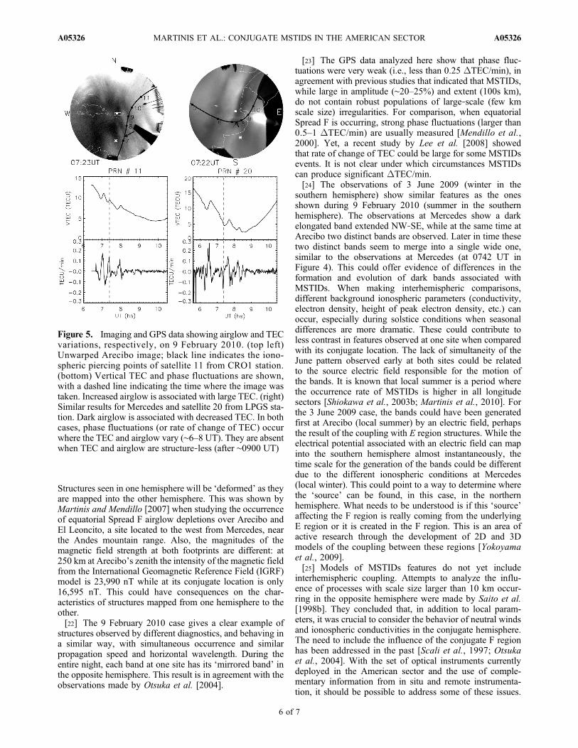
points traversing the region of depleted airglow, TECdecreases were observed. For example, Figure 5 shows tothe left Arecibo data and to the right simultaneous data forMercedes for the night of 9 February 2010. Imaging dataare shown to the top with superposed ionospheric piercingpoints of GPS PRN 11 observed by CRO1 and GPS PRN20 observed by LPGS. The arrows show the time along thetrajectory when the image was taken. The time series ofGPS TEC (center) and DTEC/min (bottom) are also shown.The vertical dashed line represents the time when the all‐sky image was taken. It is clear that the bright (dark) bandsare associated with increases (decreases) in TEC and thatrelatively weak phase fluctuations accompany both situa-tions. Even though the satellites detect TEC structures notexactly at their conjugate locations, the undulationsobserved at both hemispheres are remarkable similar. The

GPS analysis for the night of 3 June 2009 also showedphase fluctuations with negligible values, meaning thatlarge‐scale irregularities were not accompanying the band‐like structures observed by the imagers on that night.

3. Discussion and Summary

[20] The structures observed with the ASIs and GPSreceivers are common examples of processes occurring atmidlatitudes, widely referred as MSTIDs. There is still noclear mechanism for the formation of these structures but theobservation of simultaneous bands at both hemispheresprovides further proof that these processes are not simplyrelated to gravity waves occurring independently in eachhemisphere. An electrodynamical coupling must exist andcomplete theories need to address interhemispheric couplingas a key (and perhaps the most important) process.[21] When performing conjugate or interhemispheric

studies of electrodynamics at midlatitudes in the Americansector the presence of the south Atlantic magnetic anomaly(SAMA) will produce significant differences when com-pared to other longitudinal sectors. This anomaly affects theconfiguration of the magnetic field, especially in the southernhemisphere. In the Japanese‐Australian sector, the geometry(dipole‐like) dictates that mapping a circular FOV from onehemisphere to another results in another circular FOV[Otsuka et al., 2004]. In the American‐Atlantic sector, theSAMA distorts the dipolar geometry and, as a consequence,a circular FOV will not be mapped into another circle.

Figure 2. Three different nights with structures observed at both sites. (top) Arecibo images for 3 June2009, 21 September 2009, and 9 February 2010. The corresponding images obtained within a few min-utes at Mercedes are shown to the bottom. Fences, antenna, and light‐blocking elements appear to the eastin Arecibo’s imager. The Mercedes imager also shows blocking elements added to avoid light contami-nation from the cities of Buenos Aires and Mercedes. These images show full 180°FOV data.


4 of 7

Figure 3. (top) Unwarped images (i.e., converted into geographical coordinates), indicated schemati-cally by circles in Figure 1, for Arecibo images on the night of 9 February 2010. North is at the topof each image and east to the right. (bottom) Simultaneous images obtained with the Mercedes all‐skyimager. Asterisks in each image represent the geomagnetically conjugate point of the opposite hemisphereimager’s zenith location. Thus, structures observed at zenith with one imager are seen above the asteriskin the conjugate imager. The bright feature to the east at Mercedes is the Moon. These images use 160°FOV data, omitting the last 10° of zenith angle data shown in Figure 2.

Figure 4. Same format as in Figure 3 but for the night of 3 June 2009. Images at Mercedes have beenprocessed to subtract the Milky Way that is particularly prominent during this season. Notice that in eachvertical pair of simultaneous images, if a bright or dark feature falls at one site’s zenith (marked withwhite dots), the same feature is seen at its conjugate point (marked with white asterisks for Mercedes andblack asterisks for Arecibo) in the other imager.


5 of 7

Structures seen in one hemisphere will be ‘deformed’ as theyare mapped into the other hemisphere. This was shown byMartinis and Mendillo [2007] when studying the occurrenceof equatorial Spread F airglow depletions over Arecibo andEl Leoncito, a site located to the west from Mercedes, nearthe Andes mountain range. Also, the magnitudes of themagnetic field strength at both footprints are different: at250 km at Arecibo’s zenith the intensity of the magnetic fieldfrom the International Geomagnetic Reference Field (IGRF)model is 23,990 nT while at its conjugate location is only16,595 nT. This could have consequences on the char-acteristics of structures mapped from one hemisphere to theother.[22] The 9 February 2010 case gives a clear example of

structures observed by different diagnostics, and behaving ina similar way, with simultaneous occurrence and similarpropagation speed and horizontal wavelength. During theentire night, each band at one site has its ‘mirrored band’ inthe opposite hemisphere. This result is in agreement with theobservations made by Otsuka et al. [2004].

[23] The GPS data analyzed here show that phase fluc-tuations were very weak (i.e., less than 0.25 DTEC/min), inagreement with previous studies that indicated that MSTIDs,while large in amplitude (∼20–25%) and extent (100s km),do not contain robust populations of large‐scale (few kmscale size) irregularities. For comparison, when equatorialSpread F is occurring, strong phase fluctuations (larger than0.5–1 DTEC/min) are usually measured [Mendillo et al.,2000]. Yet, a recent study by Lee et al. [2008] showedthat rate of change of TEC could be large for some MSTIDsevents. It is not clear under which circumstances MSTIDscan produce significant DTEC/min.[24] The observations of 3 June 2009 (winter in the

southern hemisphere) show similar features as the onesshown during 9 February 2010 (summer in the southernhemisphere). The observations at Mercedes show a darkelongated band extended NW‐SE, while at the same time atArecibo two distinct bands are observed. Later in time thesetwo distinct bands seem to merge into a single wide one,similar to the observations at Mercedes (at 0742 UT inFigure 4). This could offer evidence of differences in theformation and evolution of dark bands associated withMSTIDs. When making interhemispheric comparisons,different background ionospheric parameters (conductivity,electron density, height of peak electron density, etc.) canoccur, especially during solstice conditions when seasonaldifferences are more dramatic. These could contribute toless contrast in features observed at one site when comparedwith its conjugate location. The lack of simultaneity of theJune pattern observed early at both sites could be relatedto the source electric field responsible for the motion ofthe bands. It is known that local summer is a period wherethe occurrence rate of MSTIDs is higher in all longitudesectors [Shiokawa et al., 2003b; Martinis et al., 2010]. Forthe 3 June 2009 case, the bands could have been generatedfirst at Arecibo (local summer) by an electric field, perhapsthe result of the coupling with E region structures. While theelectrical potential associated with an electric field can mapinto the southern hemisphere almost instantaneously, thetime scale for the generation of the bands could be differentdue to the different ionospheric conditions at Mercedes(local winter). This could point to a way to determine wherethe ‘source’ can be found, in this case, in the northernhemisphere. What needs to be understood is if this ‘source’affecting the F region is really coming from the underlyingE region or it is created in the F region. This is an area ofactive research through the development of 2D and 3Dmodels of the coupling between these regions [Yokoyamaet al., 2009].[25] Models of MSTIDs features do not yet include

interhemispheric coupling. Attempts to analyze the influ-ence of processes with scale size larger than 10 km occur-ring in the opposite hemisphere were made by Saito et al.[1998b]. They concluded that, in addition to local param-eters, it was crucial to consider the behavior of neutral windsand ionospheric conductivities in the conjugate hemisphere.The need to include the influence of the conjugate F regionhas been addressed in the past [Scali et al., 1997; Otsukaet al., 2004]. With the set of optical instruments currentlydeployed in the American sector and the use of comple-mentary information from in situ and remote instrumenta-tion, it should be possible to address some of these issues.

Figure 5. Imaging and GPS data showing airglow and TECvariations, respectively, on 9 February 2010. (top left)Unwarped Arecibo image; black line indicates the iono-spheric piercing points of satellite 11 from CRO1 station.(bottom) Vertical TEC and phase fluctuations are shown,with a dashed line indicating the time where the image wastaken. Increased airglow is associated with large TEC. (right)Similar results for Mercedes and satellite 20 from LPGS sta-tion. Dark airglow is associated with decreased TEC. In bothcases, phase fluctuations (or rate of change of TEC) occurwhere the TEC and airglow vary (∼6–8 UT). They are absentwhen TEC and airglow are structure‐less (after ∼0900 UT)


6 of 7

In particular, it needs to be determined if the band‐likestructures always appear simultaneously in both hemispheresand under which conditions they show significant iono-spheric irregularities. During the first year of observationsmost of the MSTIDs occurred simultaneously at both sites.[26] A proper and complete understanding of ionospheric

processes occurring at midlatitudes, such as MEFs, MSTIDs,and midlatitude spread F, will be obtained when observa-tions, as well as modeling, from the conjugate hemisphereare carefully taken into account.

[27] Acknowledgments. This work was supported in part by grantsfrom the Office of Naval Research, the National Science Foundation, andseed research funds from the Center for Space Physics at Boston University(BU). We thank Raul Garcia and Jonathan Friedman from the AreciboObservatory for their continuous assistance in the operation of the imagingsystem. We acknowledge the collaboration of Miguel De Laurenti, directorof the Mercedes Observatory, for his help in the installation and operationof the all‐sky imager. Data analysis assistance was provided by BU under-graduate Paul Zablowski.[28] Robert Lysak thanks the reviewer for their assistance in evaluating

this paper.

ReferencesAarons, J., M. Mendillo, R. Yantosca, and E. Kudeki (1996), GPS phasefluctuations in the equatorial region during the MISETA 1994 campaign,J. Geophys. Res., 101(A12), 26,851–26,862, doi:10.1029/96JA00981.

Behnke, R. A. (1979), F layer height bands in the nocturnal ionosphereover Arecibo, J. Geophys. Res., 84(A3), 974–978, doi:10.1029/JA084iA03p00974.

Bowman, G. G. (2001), A comparison of nighttime TID characteristicsbetween equatorial‐ionospheric‐anomaly crest and midlatitude regions,related to spread F occurrence, J. Geophys. Res., 106(A2), 1761–1769,doi:10.1029/2000JA900123.

Candido, C., A. A. Pimenta, J. A. Bittencourt, and F. Becker‐Guedes(2008), Statistical analysis of the occurrence of medium‐scale travelingionospheric disturbances over Brazilian low latitudes using OI 630.0 nmemission all‐sky images, Geophys. Res. Lett., 35, L17105, doi:10.1029/2008GL035043.

Garcia, F., M. Kelley, J. Makela, and C.‐S. Huang (2000), Airglow obser-vations of mesoscale low‐velocity traveling ionospheric disturbances atmidlatitudes, J. Geophys. Res., 105(A8), 18,407–18,415, doi:10.1029/1999JA000305.

Hunsucker, R. D. (1982), Atmospheric gravity waves generated in thehigh‐latitude ionosphere: A review, Rev. Geophys., 20, 293–315,doi:10.1029/RG020i002p00293.

Kelley, M., J. Makela, A. Saito, N. Aponte, M. Sulzer, and S. Gonzalez(2000), On the electrical structure of airglow depletion/height layer bandsover Arecibo, Geophys. Res. Lett., 27(18), 2837–2840, doi:10.1029/2000GL000024.

Lee, C. C., Y. A. Liou, Y. Otsuka, F. D. Chu, T. K. Yeh, K. Hoshinoo, andK. Matunaga (2008), Nighttime medium‐scale traveling ionospheric dis-turbances detected by network GPS receivers in Taiwan, J. Geophys.Res., 113, A12316, doi:10.1029/2008JA013250.

Martinis, C., and M. Mendillo (2007), Equatorial spread F‐related airglowdepletions at Arecibo and conjugate observations, J. Geophys. Res., 112,A10310, doi:10.1029/2007JA012403.

Martinis, C., J. Baumgardner, S. M. Smith, M. Colerico, and M. Mendillo(2006), Imaging science at El Leoncito, Argentina, Ann. Geophys., 24,1375–1385, doi:10.5194/angeo-24-1375-2006.

Martinis, C., J. Baumgardner, J. Wroten, and M. Mendillo (2010), Seasonaldependence ofMSTIDs obtained from 630.0 nm airglow imaging at Arecibo,Geophys. Res. Lett., 37, L11103, doi:10.1029/2010GL043569.

Mendillo, M., et al. (1997), Investigations of thermospheric‐ionosphericdynamics with 6300 Å images from the Arecibo Observatory, J. Geo-phys. Res., 102(A4), 7331–7343, doi:10.1029/96JA02786.

Mendillo, M., B. Lin, and J. Aarons (2000), The application of GPS obser-vations to equatorial aeronomy, Radio Sci., 35(3), 885–904, doi:10.1029/1999RS002208.

Miller, C., W. Swartz, M. Kelley, M. Mendillo, D. Nottingham, J. Scali,and B. Reinisch (1997), Electrodynamics of midlatitude spread F: 1.Observations of unstable, gravity wave‐induced ionospheric electricfields at tropical latitudes, J. Geophys. Res., 102(A6), 11,521–11,532,doi:10.1029/96JA03839.

Otsuka, Y., K. Shiokawa, T. Ogawa, and P. Wilkinson (2004), Geomag-netic conjugate observations of medium‐scale traveling ionospheric dis-turbances at midlatitude using all‐sky airglow imagers, Geophys. Res.Lett., 31, L15803, doi:10.1029/2004GL020262.

Pimenta, A. A., M. C. Kelley, Y. Sahai, J. A. Bittencourt, and P. R. Fagundes(2008), Thermospheric dark band structures observed in all‐sky OI 630 nmemission images over the Brazilian low‐latitude sector, J. Geophys. Res.,113, A01307, doi:10.1029/2007JA012444.

Richmond, A. D. (1995), Ionospheric electrodynamics using magnetic apexcoordinates, J. Geomag. Geoelectr., 47, 191–212.

Saito, A., T. Iyemori, M. Sugiura, N. C. Maynard, T. L. Aggson, L. H.Brace, M. Takeda, and M. Yamamoto (1995), Conjugate occurrence ofthe electric field fluctuations in the nighttime midlatitude ionosphere,J. Geophys. Res., 100(A11), 21,439–21,451, doi:10.1029/95JA01505.

Saito, A., T. Iyemori, L. G. Blomberg, M. Yamamoto, and M. Takeda(1998a), Conjugate observations of the mid‐latitude electric field fluctua-tions with the MU radar and the Freja satellite, J. Atmos. Sol. Terr. Phys.,60(1), 129–140, doi:10.1016/S1364-6826(97)00094-1.

Saito, A., T. Iyemori, and M. Takeda (1998b), Evolutionary process of10 kilometer scale irregularities in the nighttime midlatitude ionosphere,J. Geophys. Res., 103(A3), 3993–4000, doi:10.1029/97JA02517.

Scali, J., B. Reinisch, M. Kelley, C. Miller, W. Swartz, Q. Zhou, andS. Radicella (1997), Incoherent scatter radar and Digisonde observationsat tropical latitudes, including conjugate point studies, J. Geophys. Res.,102(A4), 7357–7367, doi:10.1029/96JA03519.

Shiokawa, K., Y. Otsuka, C. Ihara, T. Ogawa, and F. J. Rich (2003a),Ground and satellite observations of nighttime medium‐scale travelingionospheric disturbance at midlatitude, J. Geophys. Res., 108(A4),1145, doi:10.1029/2002JA009639.

Shiokawa, K., C. Ihara, Y. Otsuka, and T. Ogawa (2003b), Statistical studyof nighttime medium‐scale traveling ionospheric disturbances using mid-latitude airglow images, J. Geophys. Res., 108(A1), 1052, doi:10.1029/2002JA009491.

Shiokawa, K., et al. (2005), Geomagnetic conjugate observation of night-time medium‐scale and large‐scale traveling ionospheric disturbances:FRONT3 campaign, J. Geophys. Res., 110, A05303, doi:10.1029/2004JA010845.

Taylor, M., J. M. John, S. Fukao, and A. Saito (1998), Possible evidence ofgravity wave coupling into the midlatitude F region ionosphere duringthe SEEK campaign, Geophys. Res. Lett., 25, 1801–1804, doi:10.1029/97GL03448.

Yokoyama, T., D. L. Hysell, Y. Otsuka, and M. Yamamoto (2009), Three‐dimensional simulation of the coupled Perkins and Es‐layer instabilitiesin the nighttime midlatitude ionosphere, J. Geophys. Res., 114,A03308, doi:10.1029/2008JA013789.

J. Baumgardner, C. Martinis, M. Mendillo, and J. Wroten, Center forSpace Physics, Boston University, 725 Commonwealth Ave., Boston,MA 02215, USA. ([email protected])


7 of 7

all sky imaging observations of conjugate medium scale

Documents