all-optical information processing capacity of diffractive
TRANSCRIPT

1
All-Optical Information Processing Capacity of Diffractive Surfaces
Onur Kulce1,2,3,§, Deniz Mengu1,2,3,§, Yair Rivenson1,2,3, Aydogan Ozcan1,2,3,*
1 Electrical and Computer Engineering Department, University of California, Los Angeles, CA, 90095, USA
2 Bioengineering Department, University of California, Los Angeles, CA, 90095, USA
3 California NanoSystems Institute, University of California, Los Angeles, CA, 90095, USA
§ Equal contribution
* Corresponding author: [email protected]
Onur Kulce: [email protected]
Deniz Mengu: [email protected]
Yair Rivenson: [email protected]
Aydogan Ozcan: [email protected]

2
Abstract
The precise engineering of materials and surfaces has been at the heart of some of the recent
advances in optics and photonics. These advances related to the engineering of materials with new
functionalities have also opened up exciting avenues for designing trainable surfaces that can
perform computation and machine learning tasks through light-matter interactions and diffraction.
Here, we analyse the information processing capacity of coherent optical networks formed by
diffractive surfaces that are trained to perform an all-optical computational task between a given
input and output field-of-view. We show that the dimensionality of the all-optical solution space
covering the complex-valued transformations between the input and output fields-of-view is
linearly proportional to the number of diffractive surfaces within the optical network, up to a limit
that is dictated by the extent of the input and output fields-of-view. Deeper diffractive networks
that are composed of larger numbers of trainable surfaces can cover a higher-dimensional subspace
of the complex-valued linear transformations between a larger input field-of-view and a larger
output field-of-view and exhibit depth advantages in terms of their statistical inference, learning
and generalization capabilities for different image classification tasks when compared with a single
trainable diffractive surface. These analyses and conclusions are broadly applicable to various
forms of diffractive surfaces, including, e.g., plasmonic and/or dielectric-based metasurfaces and
flat optics, which can be used to form all-optical processors.

3
1. Introduction
The ever-growing area of engineered materials has empowered the design of novel components
and devices that can interact with and harness electromagnetic waves in unprecedented and unique
ways, offering various new functionalities 1–14. Owing to the precise control of material structure
and properties as well as the associated light-matter interaction at different scales, these engineered
material systems, including, e.g., plasmonics, metamaterials/metasurfaces and flat optics, have led
to fundamentally new capabilities in the imaging and sensing fields, among others 15–24. Optical
computing and information processing constitute yet another area that has harnessed engineered
light-matter interactions to perform computational tasks using wave optics and the propagation of
light through specially devised materials25–38. These approaches and many others highlight the
emerging uses of trained materials and surfaces as the workhorse of optical computation.
Here, we investigate the information processing capacity of trainable diffractive surfaces to shed
light on their computational power and limits. An all-optical diffractive network is physically
formed by a number of diffractive layers/surfaces and the free-space propagation between them
(see Fig. 1a). Individual transmission and/or reflection coefficients (i.e., neurons) of diffractive
surfaces are adjusted or trained to perform a desired input-output transformation task as the light
diffracts through these layers. Trained with deep-learning-based error back-propagation methods,
these diffractive networks have been shown to perform machine learning tasks such as image
classification and deterministic optical tasks including, e.g., wavelength demultiplexing, pulse
shaping and imaging38–44.
The forward model of a diffractive optical network can be mathematically formulated as a
complex-valued matrix operator that multiplies an input field vector to create an output field vector
at the detector plane/aperture. This operator is designed/trained using, e.g., deep learning to
transform a set of complex fields (forming, e.g., the input data classes) at the input aperture of the
optical network into another set of corresponding fields at the output aperture (forming, e.g., the
data classification signals) and is physically created through the interaction of the input light with
the designed diffractive surfaces as well as free-space propagation within the network (Fig. 1a).
In this paper, we investigate the dimensionality of the all-optical solution space that is covered by
a diffractive network design as a function of the number of diffractive surfaces, the number of
neurons per surface, and the size of the input and output fields-of-view. With our theoretical and
numerical analysis, we show that the dimensionality of the transformation solution space that can
be accessed through the task-specific design of a diffractive network is linearly proportional to the
number of diffractive surfaces, up to a limit that is governed by the extent of the input and output
fields-of-view. Stated differently, adding new diffractive surfaces into a given network design
increases the dimensionality of the solution space that can be all-optically processed by the
diffractive network until it reaches the linear transformation capacity dictated by the input and
output apertures (Fig. 1a). Beyond this limit, the addition of new trainable diffractive surfaces into
the optical network can cover a higher-dimensional solution space over larger input and output
fields-of-view, extending the space-bandwidth product of the all-optical processor.

4
Our theoretical analysis further reveals that, in addition to increasing the number of diffractive
surfaces within a network, another strategy to increase the all-optical processing capacity of a
diffractive network is to increase the number of trainable neurons per diffractive surface. However,
our numerical analysis involving different image classification tasks demonstrates that this strategy
of creating a higher-numerical-aperture (NA) optical network for all-optical processing of the input
information is not as effective as increasing the number of diffractive surfaces in terms of the blind
inference and generalization performance of the network. Overall, our theoretical and numerical
analyses support each other, revealing that deeper diffractive networks with larger numbers of
trainable diffractive surfaces exhibit depth advantages in terms of their statistical inference and
learning capabilities compared with a single trainable diffractive surface.
The presented analyses and conclusions are generally applicable to the design and investigation of
various coherent all-optical processors formed by diffractive surfaces such as, e.g., metamaterials,
plasmonic or dielectric-based metasurfaces, and flat-optics-based designer surfaces that can form
information processing networks to execute a desired computational task between an input and
output aperture.
2. Results
2.1. Theoretical Analysis of the Information Processing Capacity of Diffractive Surfaces
Let the 𝒙 and 𝒚 vectors represent the sampled optical fields (including the phase and amplitude
information) at the input and output apertures, respectively. We assume that the sizes of 𝒙 and 𝒚
are 𝑁𝑖 × 1 and 𝑁𝑜 × 1, defined by the input and output fields-of-view, respectively (see Fig. 1a);
these two quantities, 𝑁𝑖 and 𝑁𝑜, are simply proportional to the space-bandwidth product of the
input field and the output field at the input and output apertures of the diffractive network,
respectively. Outside the input field-of-view (FOV) defined by 𝑁𝑖, the rest of the points within the
input plane do not transmit light or any information to the diffractive network, i.e., they are
assumed to be blocked by, for example, an aperture. In a diffractive optical network composed of
transmissive and/or reflective surfaces that rely on linear optical materials, these vectors are related
to each other by 𝑨𝒙 = 𝒚, where 𝑨 represents the combined effects of the free-space wave
propagation and the transmission through (or reflection off of) the diffractive surfaces, where the
size of 𝑨 is 𝑁𝑜 × 𝑁𝑖. The matrix 𝑨 can be considered the mathematical operator that represents the
all-optical processing of the information carried by the input complex field (within the input field-
of-view/aperture), delivering the processing results to the desired output field-of-view.
Here, we prove that an optical network having a larger number of diffractive surfaces or trainable
neurons can generate a richer set for the transformation matrix 𝑨 up to a certain limit within the
set of all complex-valued matrices with size 𝑁𝑜 × 𝑁𝑖. Therefore, this section analytically
investigates the all-optical information processing capacity of diffractive networks composed of
diffractive surfaces. The input field is assumed to be monochromatic, spatially and temporally
coherent with an arbitrary polarization state, and the diffractive surfaces are assumed to be linear,
without any coupling to other states of polarization, which is ignored.

5
Let 𝑯𝒅 be an 𝑁 × 𝑁 matrix, which represents the Rayleigh-Sommerfeld diffraction between two
fields specified over parallel planes that are axially separated by a distance 𝑑. Since 𝑯𝒅 is created
from the free-space propagation convolution kernel, it is a Toeplitz matrix. Throughout the paper,
without loss of generality, we assume that 𝑁𝑖 = 𝑁𝑜 = 𝑁𝐹𝑂𝑉, 𝑁 ≥ 𝑁𝐹𝑂𝑉 and that the diffractive
surfaces are separated by free space, i.e., the refractive index surrounding the diffractive layers is
taken as n = 1. We also assume that the optical fields include only the propagating modes, i.e.,
travelling waves; stated differently, the evanescent modes along the propagation direction are not
included in our model since 𝑑 ≥ λ (Fig. 1b). With this assumption, we choose the sampling period
of the discretized complex fields to be λ/2, where λ is the wavelength of the monochromatic input
field. Accordingly, the eigenvalues of 𝑯𝒅 are in the form 𝑒𝑗𝑘𝑧𝑑 for 0 ≤ 𝑘𝑧 ≤ 𝑘𝑜, where 𝑘𝑜 is the
wavenumber of the optical field45.
Furthermore, let 𝑻𝒌 be an 𝑁𝐿𝑘 × 𝑁𝐿𝑘 matrix, which represents the 𝑘th diffractive surface/layer in
the network model, where 𝑁𝐿𝑘 is the number of neurons in the corresponding diffractive surface;
for a diffractive network composed of K surfaces, without loss of generality we assume
min(𝑁𝐿1, 𝑁𝐿2, … , 𝑁𝐿𝐾) ≥ 𝑁𝐹𝑂𝑉. Based on these definitions, the elements of 𝑻𝒌 are nonzero only
along its main diagonal entries. These diagonal entries represent the complex-valued transmittance
(or reflectance) values (i.e., the optical neurons) of the associated diffractive surface, with a
sampling period of λ/2. Furthermore, each diffractive surface defined by a given transmittance
matrix is assumed to be surrounded by a blocking layer within the same plane to avoid any optical
communication between the layers without passing through an intermediate diffractive surface.
This formalism embraces any form of diffractive surface, including, e.g., plasmonic or dielectric-
based metasurfaces. Even if the diffractive surface has deeply sub-wavelength structures, with a
much smaller sampling period compared to λ/2 and many more degrees of freedom (M) compared
to 𝑁𝐿𝑘, the information processing capability of a diffractive surface within a network is limited to
propagating modes since 𝑑 ≥ λ, which restricts the effective number of neurons per layer to 𝑁𝐿𝑘
(Fig. 1b). In other words, since we assume that only propagating modes can reach the subsequent
diffractive surfaces within the optical diffractive network, the sampling period (and hence, the
neuron size) of λ/2 is sufficient to represent these propagating modes in air46. According to
Shannon’s sampling theorem, since the spatial frequency band of the propagating modes in air is
restricted to the (−1/λ, 1/λ) interval, a neuron size that is smaller than λ/2 leads to oversampling
and over-utilization of the optical neurons of a given diffractive surface. On the other hand, if one
aims to control and engineer the evanescent modes, then a denser sampling period on each
diffractive surface is needed, which might be useful to build diffractive networks that have 𝑑 ≪ λ. In this near-field diffractive network, the enormously rich degrees of freedom enabled by various
metasurface designs with 𝑀 ≫ 𝑁𝐿𝑘 can be utilized to provide full and independent control of the
phase and amplitude coefficients of each individual neuron of a diffractive surface.
The underlying physical process of how the light is modulated by an optical neuron may vary in
different diffractive surface designs. In a dielectric-material-based transmissive design, for
example, phase modulation can be achieved by slowing down the light inside the material, where
the thickness of an optical neuron determines the amount of phase shift that the light beam
undergoes. Alternatively, liquid-crystal (LC)-based spatial light modulators (SLMs) or flat-optics-
based metasurfaces can also be employed as part of a diffractive network to generate the desired
phase and/or amplitude modulation on the transmitted or reflected light9,47.

6
Starting from Section 2.1.1, we investigate the physical properties of 𝑨, generated by different
numbers of diffractive surfaces and trainable neurons. In this analysis, without loss of generality,
each diffractive surface is assumed to be transmissive, following the schematics shown in Fig. 1a,
and its extension to reflective surfaces is straightforward and does not change our conclusions.
Finally, multiple (back and forth) reflections within a diffractive network composed of different
layers are ignored in our analysis, as these are much weaker processes compared to the forward
propagating modes.
2.1.1. Analysis of a single diffractive surface
The input-output relationship for a single diffractive surface that is placed between an input and
an output FOV (Fig. 1a) can be written as:
where d1 ≥ λ and d2 ≥ λ represent the axial distance between the input plane and the diffractive
surface, and the axial distance between the diffractive surface and the output plane, respectively.
Here we also assume that d1 ≠ d2; the Supplementary Information, Section S5 discusses the special
case of d1 = d2. Since there is only one diffractive surface in the network, we denote the
transmittance matrix as 𝑻𝟏, the size of which is 𝑁𝐿1 × 𝑁𝐿1, where L1 represents the diffractive
surface. Here, 𝑯𝒅𝟏′ is an 𝑁𝐿1 × 𝑁𝐹𝑂𝑉 matrix that is generated from the 𝑁𝐿1 × 𝑁𝐿1 propagation
matrix 𝑯𝒅𝟏 by deleting the appropriately chosen 𝑁𝐿1 − 𝑁𝐹𝑂𝑉-many columns. The positions of the
deleted columns correspond to the zero transmission values at the input plane that lie outside the
input field-of-view or aperture defined by 𝑁𝑖 = 𝑁𝐹𝑂𝑉 (Fig. 1a), i.e., not included in 𝒙. Similarly,
𝑯𝒅𝟐′ is an 𝑁𝐹𝑂𝑉 × 𝑁𝐿1 matrix that is generated from the 𝑁𝐿1 × 𝑁𝐿1 propagation matrix 𝑯𝒅𝟐 by
deleting the appropriately chosen 𝑁𝐿1 − 𝑁𝐹𝑂𝑉-many rows, which correspond to the locations
outside the output FOV or aperture defined by 𝑁𝑜 = 𝑁𝐹𝑂𝑉 in Fig. 1a; this means that the output
field is calculated only within the desired output aperture. As a result, 𝑯𝒅𝟏′ and 𝑯𝒅𝟐
′ have a rank of
𝑁𝐹𝑂𝑉.
To investigate the information processing capacity of 𝑨𝟏 based on a single diffractive surface, we
vectorize this matrix in the column order and denote it as 𝑣𝑒𝑐(𝑨𝟏) = 𝒂𝟏 48. Next, we show that
the set of possible 𝒂𝟏 vectors forms a min(𝑁𝐿1, 𝑁𝐹𝑂𝑉2 )-dimensional subset of an 𝑁𝐹𝑂𝑉
2 -dimensional
complex-valued vector field. The vector, 𝒂𝟏, can be written as:
where the superscript 𝑇 and ⊗ denote the transpose operation and Kronecker product,
respectively48. Here, the size of 𝑯𝒅𝟏′𝑇 ⊗𝑯𝒅𝟐
′ is 𝑁𝐹𝑂𝑉2 × 𝑁𝐿1
2 , and it is a full-rank matrix with rank
𝑁𝐹𝑂𝑉2 . In Equation 2, 𝑣𝑒𝑐(𝑻𝟏) = 𝒕𝟏 has at most 𝑁𝐿1 controllable/adjustable complex-valued
entries, which physically represent the neurons of the diffractive surface, and the rest of its entries
are all zero. These transmission coefficients lead to a linear combination of 𝑁𝐿1-many vectors of
𝑯𝒅𝟏′𝑇 ⊗𝑯𝒅𝟐
′ , where d1 ≠ d2 ≠ 0. If 𝑁𝐿1 ≤ 𝑁𝐹𝑂𝑉2 , these vectors subject to the linear combination are
𝒚 = 𝑯𝒅𝟐′ 𝑻𝟏𝑯𝒅𝟏
′ 𝒙 = 𝑨𝟏𝒙 1
𝑣𝑒𝑐(𝑨𝟏) = 𝒂𝟏 = 𝑣𝑒𝑐(𝑯𝒅𝟐′ 𝑻𝟏𝑯𝒅𝟏
′ )
= (𝑯𝒅𝟏′𝑇 ⊗𝑯𝒅𝟐
′ )𝑣𝑒𝑐(𝑻𝟏)
= (𝑯𝒅𝟏′𝑇 ⊗𝑯𝒅𝟐
′ )𝒕𝟏
2

7
linearly independent (see the Supplementary Information Section S4.1 and Supplementary Figure
S1). Hence, the set of resulting 𝒂𝟏 vectors generated by Equation 2 forms an 𝑁𝐿1-dimensional
subspace of the 𝑁𝐹𝑂𝑉2 -dimensional complex-valued vector space. On the other hand, if 𝑁𝐿1 >
𝑁𝐹𝑂𝑉2 , then the vectors in the linear combination start to become dependent on each other. In this
case of 𝑁𝐿1 > 𝑁𝐹𝑂𝑉2 , the dimensionality of the set of possible vector fields is limited to 𝑁𝐹𝑂𝑉
2 (also
see Supplementary Figure S1).
This analysis demonstrates that the set of complex field transformation vectors that can be
generated by a single diffractive surface that connects a given input and output FOV constitutes a
min(𝑁𝐿1, 𝑁𝐹𝑂𝑉2 )-dimensional subspace of an 𝑁𝐹𝑂𝑉
2 -dimensional complex-valued vector space.
These results are based on our earlier assumption that d1 ≥ λ, d2 ≥ λ and d1 ≠ d2. For the special
case of d1 = d2 ≥ λ, the upper limit of the dimensionality of the solution space that can be generated
by a single diffractive surface (K = 1) is reduced from 𝑁𝐹𝑂𝑉2 to (𝑁𝐹𝑂𝑉
2 + 𝑁𝐹𝑂𝑉)/2 due to the
combinatorial symmetries that exist in the optical path for d1 = d2 (see the Supplementary
Information, Section S5).
2.1.2. Analysis of an optical network formed by two diffractive surfaces
Here, we consider an optical network with two different (trainable) diffractive surfaces (K=2),
where the input-output relation can be written as:
𝑁𝑥 = max(𝑁𝐿1, 𝑁𝐿2) determines the sizes of the matrices in Equation 3, where 𝑁𝐿1 and 𝑁𝐿2
represent the number of neurons in the first and second diffractive surfaces, respectively; d1, d2
and d3 represent the axial distances between the diffractive surfaces (see Fig. 1a). Accordingly, the
sizes of 𝑯𝒅𝟏′ , 𝑯𝒅𝟐 and 𝑯𝒅𝟑
′ become 𝑁𝑥 × 𝑁𝐹𝑂𝑉, 𝑁𝑥 × 𝑁𝑥 and 𝑁𝐹𝑂𝑉 × 𝑁𝑥, respectively. Since we
have already assumed that min(𝑁𝐿1, 𝑁𝐿2) ≥ 𝑁𝐹𝑂𝑉, 𝑯𝒅𝟏′ and 𝑯𝒅𝟑
′ can be generated from the
corresponding 𝑁𝑥 × 𝑁𝑥 propagation matrices by deleting the appropriate columns and rows, as
described in Section 2.1.1. Because 𝑯𝒅𝟐 has a size of 𝑁𝑥 × 𝑁𝑥, there is no need to delete any rows
or columns from the associated propagation matrix. Although both 𝑻𝟏 and 𝑻𝟐 have a size of 𝑁𝑥 ×𝑁𝑥, the one corresponding to the diffractive surface that contains the smaller number of neurons
has some zero values along its main diagonal indices. The number of these zeros is 𝑁𝑥 −min(𝑁𝐿1, 𝑁𝐿2).
Similar to the analysis reported in Section 2.1.1, the vectorization of 𝑨𝟐 reveals:
𝒚 = 𝑯𝒅𝟑′ 𝑻𝟐𝑯𝒅𝟐𝑻𝟏𝑯𝒅𝟏
′ 𝒙 = 𝑨𝟐𝒙 3
𝑣𝑒𝑐(𝑨𝟐) = 𝒂𝟐 = 𝑣𝑒𝑐(𝑯𝒅𝟑′ 𝑻𝟐𝑯𝒅𝟐𝑻𝟏𝑯𝒅𝟏
′ )
= (𝑯𝒅𝟏′𝑇 ⊗𝑯𝒅𝟑
′ )𝑣𝑒𝑐(𝑻𝟐𝑯𝒅𝟐𝑻𝟏)
= (𝑯𝒅𝟏′𝑇 ⊗𝑯𝒅𝟑
′ )(𝑻𝟏𝑇⊗𝑻𝟐)𝑣𝑒𝑐(𝑯𝒅𝟐)
= (𝑯𝒅𝟏′𝑇 ⊗𝑯𝒅𝟑
′ )(𝑻𝟏⊗𝑻𝟐)𝑣𝑒𝑐(𝑯𝒅𝟐)
= (𝑯𝒅𝟏′𝑇 ⊗𝑯𝒅𝟑
′ )(𝑻𝟏⊗𝑻𝟐)𝒉𝒅𝟐
= (𝑯𝒅𝟏′𝑇 ⊗𝑯𝒅𝟑
′ )�̂�𝒅𝟐𝑑𝑖𝑎𝑔(𝑻𝟏⊗𝑻𝟐)
= (𝑯𝒅𝟏′𝑇 ⊗𝑯𝒅𝟑
′ )�̂�𝒅𝟐𝒕𝟏𝟐
4

8
where �̂�𝒅𝟐 is an 𝑁𝑥2 × 𝑁𝑥
2 matrix that has nonzero entries only along its main diagonal locations.
These entries are generated from 𝑣𝑒𝑐(𝑯𝒅𝟐) = 𝒉𝒅𝟐 such that �̂�𝒅𝟐 [𝑖, 𝑖] = 𝒉𝒅𝟐[𝑖]. Since the
𝑑𝑖𝑎𝑔(⋅) operator forms a vector from the main diagonal entries of its input matrix, the vector 𝒕𝟏𝟐 =𝑑𝑖𝑎𝑔(𝑻𝟏⊗𝑻𝟐) is generated such that 𝒕𝟏𝟐[𝑖] = (𝑻𝟏⊗𝑻𝟐)[𝑖, 𝑖]. The equality (𝑻𝟏⊗𝑻𝟐)𝒉𝒅𝟐 =
�̂�𝒅𝟐𝒕𝟏𝟐 stems from the fact that the nonzero elements of 𝑻𝟏⊗𝑻𝟐 are located only along its main
diagonal entries.
In Equation 4, 𝑯𝒅𝟏′𝑇 ⊗𝑯𝒅𝟑
′ has rank 𝑁𝐹𝑂𝑉2 . Since all the diagonal elements of �̂�𝒅𝟐are nonzero, it
has rank 𝑁𝑥2. As a result, (𝑯𝒅𝟏
𝑇 ⊗𝑯𝒅𝟑)�̂�𝒅𝟐 is a full-rank matrix with rank 𝑁𝐹𝑂𝑉2 . Additionally, the
nonzero elements of 𝒕𝟏𝟐 take the form 𝑡𝑖𝑗 = 𝑡1,𝑖𝑡2,𝑗, where 𝑡1,𝑖 and 𝑡2,𝑗 are the trainable/adjustable
complex transmittance values of the 𝑖th neuron of the 1st diffractive surface and the 𝑗th neuron of
the 2nd diffractive surface, respectively, for 𝑖 ∈ {1,2, … ,𝑁𝐿1} and 𝑗 ∈ {1,2, … , 𝑁𝐿2}. Then, the set
of possible 𝒂𝟐 vectors (Equation 4) can be written as:
where 𝒉𝒊𝒋 is the corresponding column vector of (𝑯𝒅𝟏′𝑇 ⊗𝑯𝒅𝟑
′ )�̂�𝒅𝟐.
Equation 5 is in the form of a complex-valued linear combination of 𝑁𝐿1𝑁𝐿2-many complex-valued
vectors, 𝒉𝒊𝒋. Since we assume min(𝑁𝐿1, 𝑁𝐿2) ≥ 𝑁𝐹𝑂𝑉, these vectors necessarily form a linearly
dependent set of vectors and this restricts the dimensionality of the vector space to 𝑁𝐹𝑂𝑉2 .
Moreover, due to the coupling of the complex-valued transmittance values of the two diffractive
surfaces (𝑡𝑖𝑗 = 𝑡1,𝑖𝑡2,𝑗) in Equation 5, the dimensionality of the resulting set of 𝒂𝟐 vectors can even
go below 𝑁𝐹𝑂𝑉2 , despite 𝑁𝐿1𝑁𝐿2 ≥ 𝑁𝐹𝑂𝑉
2 . In fact, in the Materials and Methods section, we show
that the set of 𝒂𝟐 vectors can form an 𝑁𝐿1+𝑁𝐿2 − 1-dimensional subspace of the 𝑁𝐹𝑂𝑉2 -
dimensional complex-valued vector space and can be written as:
where 𝒃𝒌 represents length-𝑁𝐹𝑂𝑉2 linearly independent vectors and 𝑐𝑘 represents complex-valued
coefficients, generated through the coupling of the transmittance values of the two independent
diffractive surfaces. The relationship between Equations 5 and 6 is also presented as a pseudo-
code in Table 1; see also Supplementary Tables S1-S3 and Supplementary Figure S2.
These analyses reveal that by using a diffractive optical network composed of two different
trainable diffractive surfaces (with neurons 𝑁𝐿1, 𝑁𝐿2), it is possible to generate an all-optical
solution that spans an 𝑁𝐿1+𝑁𝐿2 − 1 dimensional subspace of an 𝑁𝐹𝑂𝑉2 -dimensional complex-
valued vector space. As a special case, if we assume 𝑁 = 𝑁𝐿1 = 𝑁𝐿2 = 𝑁𝑖 = 𝑁𝑜 = 𝑁𝐹𝑂𝑉, the
resulting set of complex-valued linear transformation vectors forms a 2𝑁 − 1 dimensional
subspace of an 𝑁2-dimensional vector field. The Supplementary Information (Section S1 and
Table S1) also provides a coefficient and basis vector generation algorithm, independently
𝒂𝟐 =∑𝑡𝑖𝑗𝒉𝒊𝒋𝑖,𝑗
5
𝒂𝟐 = ∑ 𝑐𝑘𝒃𝒌
𝑁𝐿1+𝑁𝐿2−1
𝑘=1
6

9
reaching the same conclusion that this special case forms a 2𝑁 − 1 dimensional subspace of an
𝑁2-dimensional vector field. The upper limit of the solution space dimensionality that can be
achieved by a two-layered diffractive network is 𝑁𝐹𝑂𝑉2 , which is dictated by the input and output
fields-of-view between which the diffractive network is positioned.
In summary, these analyses show that the dimensionality of the all-optical solution space covered
by two trainable diffractive surfaces (K = 2) positioned between a given set of input-output FOV
is given by min(𝑁𝐹𝑂𝑉2 , N𝐿1+N𝐿2 − 1). Different from K = 1 architecture, which revealed a
restricted solution space when d1 = d2 (see the Supplementary Information, Section S5), diffractive
optical networks with K=2 do not exhibit a similar restriction related to the axial distances d1, d2
and d3 (see Supplementary Figure S2).
2.1.3. Analysis of an optical network formed by three or more diffractive surfaces
Next, we consider an optical network formed by more than 2 diffractive surfaces, with neurons of
(𝑁𝐿1, 𝑁𝐿2, ⋯ , 𝑁𝐿𝐾) for each layer, where K is the number of diffractive surfaces and 𝑁𝐿𝑘 represents
the number of neurons in the kth layer. In the previous section, we showed that a two-layered
network with (𝑁𝐿1, 𝑁𝐿2) neurons has the same solution space dimensionality as that of a single-
layered, larger diffractive network having N𝐿1+N𝐿2 − 1 individual neurons. If we assume that a
third diffractive surface (𝑁𝐿3) is added to this single-layer network with N𝐿1+N𝐿2 − 1 neurons,
this becomes equivalent to a two-layered network with (𝑁𝐿1+𝑁𝐿2 − 1 , 𝑁𝐿3) neurons. Based on
Section 2.1.2, the dimensionality of the all-optical solution space covered by this diffractive
network positioned between a set of input-output fields-of-view is given by
min(𝑁𝐹𝑂𝑉2 , 𝑁𝐿1+𝑁𝐿2+𝑁𝐿3 − 2); also see Supplementary Figure S3. For the special case of
𝑁𝐿1 = 𝑁𝐿2 = 𝑁𝐿3 = 𝑁𝑖 = 𝑁𝑜 = 𝑁, Supplementary Information Section S2 and Table S2
independently illustrate that the resulting vector field is indeed a 3𝑁 − 2 dimensional subspace of
an 𝑁2-dimensional vector field.
The above arguments can be extended to a network that has K diffractive surfaces. That is, for a
multi-surface diffractive network with a neuron distribution of (𝑁𝐿1, 𝑁𝐿2, ⋯ , 𝑁𝐿𝐾), the
dimensionality of the solution space (see Fig. 2) created by this diffractive network is given by:
which forms a subspace of an 𝑁𝐹𝑂𝑉2 -dimensional vector space that covers all the complex-valued
linear transformations between the input and output fields-of-view.
The upper bound on the dimensionality of the solution space, i.e., the 𝑁𝐹𝑂𝑉2 term in Equation 7, is
heuristically imposed by the number of possible ray interactions between the input and output
fields-of-view. That is, if we consider the diffractive optical network as a black box (Fig. 1a), its
operation can be intuitively understood as controlling the phase and/or amplitude of the light rays
that are collected from the input, to be guided to the output, following a lateral grid of λ/2 at the
min(𝑁𝐹𝑂𝑉2 , [∑𝑁𝐿𝑘
𝐾
𝑘=1
] − (𝐾 − 1))
7

10
input/output fields-of-view, determined by the diffraction limit of light. The second term in
Equation 7, on the other hand, reflects the total space-bandwidth product of K successive
diffractive surfaces, one following another. To intuitively understand the (𝐾 − 1) subtraction term
in Equation 7, one can hypothetically consider the simple case of 𝑁𝐿𝑘 = 𝑁𝐹𝑂𝑉 = 1 for all K
diffractive layers; in this case, [∑ 𝑁𝐿𝑘𝐾𝑘=1 ] − (𝐾 − 1) = 1, which simply indicates that K
successive diffractive surfaces (each with 𝑁𝐿𝑘 = 1) are equivalent, as physically expected, to a
single controllable diffractive surface with 𝑁𝐿=1.
Without loss of generality, if we assume 𝑁 = 𝑁𝑘 for all the diffractive surfaces, then the
dimensionality of the linear transformation solution space created by this diffractive network will
be 𝐾𝑁 − (𝐾 − 1), provided that 𝐾𝑁 − (𝐾 − 1) ≤ 𝑁𝐹𝑂𝑉2 . The Supplementary Information
(Section S3 and Table S3) also provides an independent proof of the same conclusion. This means
that for a fixed design choice of 𝑁 neurons per diffractive surface (determined by, e.g., the
limitations of the fabrication methods or other practical considerations), adding new diffractive
surfaces to the same diffractive network linearly increases the dimensionality of the solution space
that can be all-optically processed by the diffractive network between the input/output fields-of-
view. As we further increase K such that 𝐾𝑁 − (𝐾 − 1) ≥ 𝑁𝐹𝑂𝑉2 , the diffractive network reaches
its linear transformation capacity, and adding more layers or more neurons to the network does not
further contribute to its processing power for the desired input-output fields-of-view (see Fig. 2).
However, these deeper diffractive networks that have larger numbers of diffractive surfaces (i.e.,
𝐾𝑁 − (𝐾 − 1) ≥ 𝑁𝐹𝑂𝑉2 ) can cover a solution space with a dimensionality of 𝐾𝑁 − (𝐾 − 1) over
larger input and output fields-of-view. Stated differently, for any given choice of 𝑁 neurons per
diffractive surface, deeper diffractive networks that are composed of multiple surfaces can cover
a 𝐾𝑁 − (𝐾 − 1)-dimensional subspace of all the complex-valued linear transformations between
a larger input field-of-view (𝑁′𝑖 > 𝑁𝑖) and/or a larger output field-of view (𝑁′𝑜 > 𝑁𝑜), as long as
𝐾𝑁 − (𝐾 − 1) ≤ 𝑁′𝑖𝑁′𝑜. The conclusions of this analysis are also summarized in Fig. 2.
In addition to increasing K (the number of diffractive surfaces within an optical network), an
alternative strategy to increase the all-optical processing capabilities of a diffractive network is to
increase N, the number of neurons per diffractive surface/layer. However, as we numerically
demonstrate in the next section, this strategy is not as effective as increasing the number of
diffractive surfaces since deep-learning-based design tools are relatively inefficient in utilizing all
the degrees of freedom provided by a diffractive surface with 𝑁 >> 𝑁𝑜, 𝑁𝑖. This is partially related
to the fact that high-numerical-aperture optical systems are generally more difficult to optimize
and design. Moreover, if we consider a single-layer diffractive network design with a large Nmax
(which defines the maximum surface area that can be fabricated and engineered with the desired
transmission coefficients), even for this Nmax design, the addition of new diffractive surfaces with
Nmax at each surface linearly increases the dimensionality of the solution space created by the
diffractive network, covering linear transformations over larger input and output fields-of-view,
as discussed earlier. These reflect some of the important depth advantages of diffractive optical
networks that are formed by multiple diffractive surfaces. The next section further expands on this
using a numerical analysis of diffractive optical networks that are designed for image
classification.
2.2. Numerical Analysis of Diffractive Networks
11
The previous section showed that the dimensionality of the all-optical solution space covered by
K diffractive surfaces, forming an optical network positioned between an input and output field-
of-view, is determined by min(𝑁𝐹𝑂𝑉2 , [∑ 𝑁𝐿𝑘
𝐾𝑘=1 ] − (𝐾 − 1)). However, this mathematical
analysis does not shed light on the selection or optimization of the complex transmittance (or
reflectance) values of each neuron of a diffractive network that is assigned for a given
computational task. Here, we numerically investigate the function approximation power of
multiple diffractive surfaces in the (N, K) space using image classification as a computational goal
for the design of each diffractive network. Since NFOV and N are large numbers in practice, an
iterative optimization procedure based on error back-propagation and deep learning with a desired
loss function was used to design diffractive networks and compare their performances as a function
of (N, K).
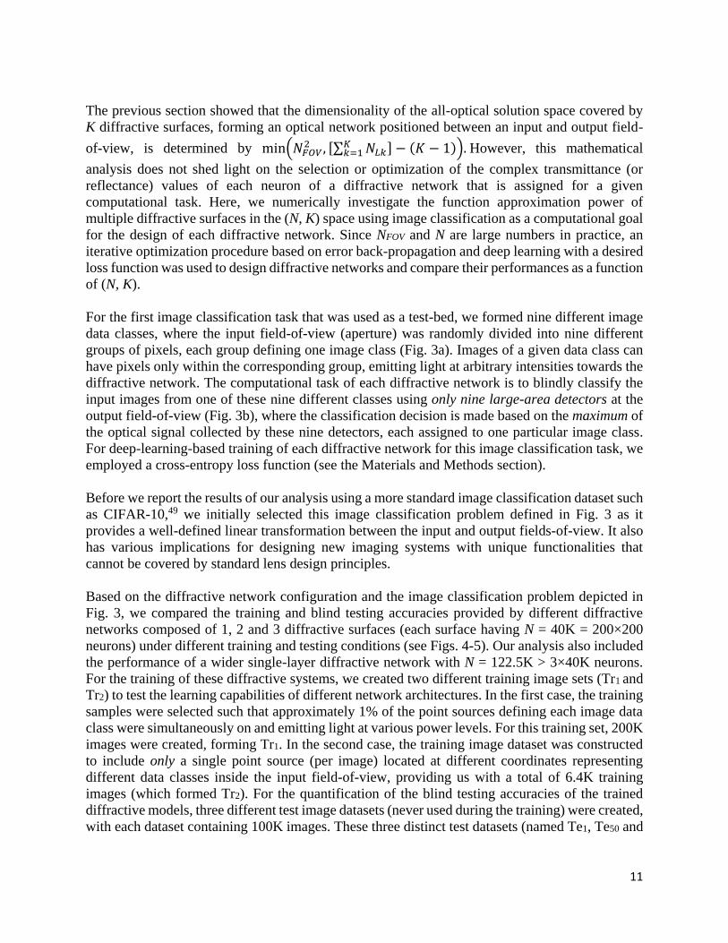
For the first image classification task that was used as a test-bed, we formed nine different image
data classes, where the input field-of-view (aperture) was randomly divided into nine different
groups of pixels, each group defining one image class (Fig. 3a). Images of a given data class can
have pixels only within the corresponding group, emitting light at arbitrary intensities towards the
diffractive network. The computational task of each diffractive network is to blindly classify the
input images from one of these nine different classes using only nine large-area detectors at the
output field-of-view (Fig. 3b), where the classification decision is made based on the maximum of
the optical signal collected by these nine detectors, each assigned to one particular image class.
For deep-learning-based training of each diffractive network for this image classification task, we
employed a cross-entropy loss function (see the Materials and Methods section).
Before we report the results of our analysis using a more standard image classification dataset such
as CIFAR-10,49 we initially selected this image classification problem defined in Fig. 3 as it
provides a well-defined linear transformation between the input and output fields-of-view. It also
has various implications for designing new imaging systems with unique functionalities that
cannot be covered by standard lens design principles.
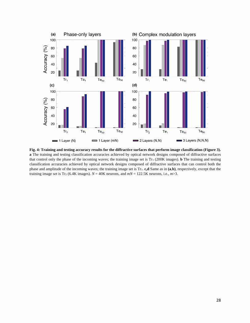
Based on the diffractive network configuration and the image classification problem depicted in
Fig. 3, we compared the training and blind testing accuracies provided by different diffractive
networks composed of 1, 2 and 3 diffractive surfaces (each surface having N = 40K = 200×200
neurons) under different training and testing conditions (see Figs. 4-5). Our analysis also included
the performance of a wider single-layer diffractive network with N = 122.5K > 3×40K neurons.
For the training of these diffractive systems, we created two different training image sets (Tr1 and
Tr2) to test the learning capabilities of different network architectures. In the first case, the training
samples were selected such that approximately 1% of the point sources defining each image data
class were simultaneously on and emitting light at various power levels. For this training set, 200K
images were created, forming Tr1. In the second case, the training image dataset was constructed
to include only a single point source (per image) located at different coordinates representing
different data classes inside the input field-of-view, providing us with a total of 6.4K training
images (which formed Tr2). For the quantification of the blind testing accuracies of the trained
diffractive models, three different test image datasets (never used during the training) were created,
with each dataset containing 100K images. These three distinct test datasets (named Te1, Te50 and

12
Te90) contain image samples that take contributions from 1% (Te1), 50% (Te50) and 90% (Te90) of
the points defining each image data class (see Fig. 3).
Figure 4 illustrates the blind classification accuracies achieved by the different diffractive network
models that we trained. We see that as the number of diffractive surfaces in the network increases,
the testing accuracies achieved by the final diffractive design improve significantly, meaning that
the linear transformation space covered by the diffractive network expands with the addition of
new trainable diffractive surfaces, in line with our former theoretical analysis. For instance, while
a diffractive image classification network with a single phase-only (complex) modulation surface
can achieve 24.48% (27.00%) for the test image set Te1, the three-layer versions of the same
architectures attain 85.2% (100.00%) blind testing accuracies, respectively (see Figs. 4a,b). Figure
5 shows the phase-only diffractive layers comprising the 1- and 3-layer diffractive optical networks
that are compared in Fig. 4a; Fig. 5 also reports some exemplary test images selected from Te1 and
Te50, along with the corresponding intensity distributions at the output planes of the diffractive
networks. The comparison between two- and three-layer diffractive systems also indicates a
similar conclusion for the test image set, Te1. However, as we increase the number of point sources
contributing to the test images, e.g., for the case of Te90, the blind testing classification accuracies
of both the two- and three-layer networks saturate at nearly 100%, indicating that the solution
space of the two-layer network already covers the optical transformation required to address this
relatively easier image classification problem set by Te90.
A direct comparison between the classification accuracies reported in Figs. 4a,c and Figs. 4b,d
further reveals that the phase-only modulation constraint relatively limits the approximation power
of the diffractive network since it places a restriction on the coefficients of the basis vectors, 𝒉𝒊𝒋.
For example, when a two-layer, phase-only diffractive network is trained with Tr1 and blindly
tested with the images of Te1, the training and testing accuracies are obtained as 78.72% and
78.44%, respectively. On the other hand, if the diffractive surfaces of the same network
architectures have independent control of the transmission amplitude and phase value of each
neuron of a given surface, the same training (Tr1) and testing (Te1) accuracy values increase to
97.68% and 97.39%, respectively.
As discussed in our earlier theoretical analysis, an alternative strategy to increase the all-optical
processing capabilities of a diffractive network is to increase N, the number of neurons per
diffractive surface. We also numerically investigated this scenario by training and testing another
diffractive image classifier with a single surface that contains 122.5K neurons, i.e., it has more
trainable neurons than the 3-layer diffractive designs reported in Fig. 4. As demonstrated in Fig.
4, although the performance of this larger/wider diffractive surface surpassed that of the previous,
narrower/smaller 1-layer designs with 40K trainable neurons, its blind testing accuracy could not
match the classification accuracies achieved by a 2-layer (2×40K neurons) network in both the
phase-only and complex modulation cases. Despite using more trainable neurons than the 2-layer
and 3-layer diffractive designs, the blind inference and generalization performance of this
larger/wider diffractive surface is worse than that of the multi-surface diffractive designs. In fact,
if we were to further increase the number of neurons in this single diffractive surface (further
increasing the effective numerical aperture of the diffractive network), the inference performance
gain due to these additional neurons that are farther away from the optical axis will asymptotically

13
go to zero since the corresponding k-vectors of these neurons carry a limited amount of optical
power for the desired transformations targeted between the input and output fields-of-view.
Another very important observation that one can make in Figs. 4c,d is that the performance
improvements due to the increasing number of diffractive surfaces are much more pronounced for
more challenging (i.e., limited) training image datasets, such as Tr2. With a significantly smaller
number of training images (6.4K images in Tr2 as opposed to 200K images in Tr1), multi-surface
diffractive networks trained with Tr2 successfully generalized to different test image datasets (Te1,
Te50 and Te90) and efficiently learned the image classification problem at hand, whereas the single-
surface diffractive networks (including the one with 122.5K trainable neurons per layer) almost
entirely failed to generalize; see, e.g., Figs. 4c,d, the blind testing accuracy values for the
diffractive models trained with Tr2.
Next, we applied our analysis to a widely used, standard image classification dataset and
investigated the performance of diffractive image classification networks comprised of one, three
and five diffractive surfaces using the CIFAR-10 image dataset49. Unlike the previous image
classification dataset (Fig. 3), the samples of CIFAR-10 contain images of physical objects, e.g.,
airplanes, birds, cats, dogs, etc., and CIFAR-10 has been widely used for quantifying the
approximation power associated with various deep neural network architectures. Here, we assume
that the CIFAR-10 images are encoded in the phase channel of the input field-of-view that is
illuminated with a uniform plane wave. For deep-learning-based training of the diffractive
classification networks, we adopted two different loss functions. The first loss function is based
on the mean-squared-error (MSE), which essentially formulates the design of the all-optical object
classification system as an image transformation/projection problem, and the second one is based
on the cross-entropy loss, which is commonly used to solve the multi-class separation problems in
the deep learning literature (refer to the Materials and Methods section for details).
The results of our analysis are summarized in Figs. 6a and 6b, which report the average blind
inference accuracies along with the corresponding standard deviations observed over the testing
of three different diffractive network models trained independently to classify the CIFAR-10 test
images using phase-only and complex-valued diffractive surfaces, respectively. The 1-, 3-, and 5-
layer phase-only (complex-valued) diffractive network architectures can attain blind classification
accuracies of 40.55∓0.10% (41.52∓0.09%), 44.47∓0.14% (45.88∓0.28%) and 45.53∓0.30%
(46.84∓0.46%), respectively, when they are trained based on the cross-entropy loss detailed in the
Materials and Methods section. On the other hand, with the use of the MSE loss, these
classification accuracies are reduced to 16.25∓0.48% (14.92∓0.26%), 29.08∓0.14%
(33.52∓0.40%) and 33.67∓0.57% (34.69∓0.11%), respectively. In agreement with the
conclusions of our previous results and the presented theoretical analysis, the blind testing
accuracies achieved by the all-optical diffractive classifiers improve with increasing number of
diffractive layers, K, independent of the loss function used and the modulation constraints imposed
on the trained surfaces (see Fig. 6).
Different from electronic neural networks, however, diffractive networks are physical machine
learning platforms with their own optical hardware; hence, practical design merits such as the
signal-to-noise ratio (SNR) and the contrast-to-noise ratio (CNR) should also be considered, as
these features can be critical for the success of these networks in various applications. Therefore,

14
in addition to the blind testing accuracies, the performance evaluation and comparison of these all-
optical diffractive classification systems involve two additional metrics that are analogous to the
SNR and CNR. The first is the classification efficiency, which we define as the ratio of the optical
signal collected by the target, ground-truth class detector, Igt, with respect to the total power
collected by all class detectors located at the output plane. The second performance metric refers
to the normalized difference between the optical signals measured by the ground-truth/correct
detector, Igt, and its strongest competitor, Isc, i.e., (𝐼𝑔𝑡 − 𝐼𝑠𝑐) / 𝐼𝑔𝑡; this optical signal contrast
metric is, in general, important since the relative level of detection noise with respect to this
difference is critical for translating the accuracies achieved by the numerical forward models to
the performance of the physically fabricated diffractive networks. Figure 6 reveals that the
improvements observed in the blind testing accuracies as a function of the number of diffractive
surfaces also apply to these two important diffractive network performance metrics, resulting from
the increased dimensionality of the all-optical solution space of the diffractive network with
increasing K. For instance, the diffractive network models presented in Fig. 6b, trained with the
cross-entropy (or MSE) loss function, provide classification efficiencies of 13.72∓0.03%
(13.98∓0.12%), 15.10∓0.08% (31.74∓0.41%) and 15.46∓0.08% (34.43∓0.28%) using complex-
valued 1-, 3- and 5-layers, respectively. Furthermore, the optical signal contrast attained by the
same diffractive network designs can be calculated as 10.83∓0.17% (9.25∓0.13%), 13.92∓0.28%
(35.23∓1.02%) and 14.88∓0.28% (38.67∓0.13%), respectively. Similar improvements are also
observed for the phase-only diffractive optical network models that are reported in Fig. 6a. These
results indicate that the increased dimensionality of the solution space with increasing K improves
the inference capacity as well as the robustness of the diffractive network models by enhancing
their optical efficiency and signal contrast.
Apart from the results and analyses reported in this section, the depth advantage of diffractive
networks has been empirically shown in the literature for some other applications and datasets,
such as, e.g., image classification38,40 and optical spectral filter design42.
3. Discussion
In a diffractive optical design problem, it is not guaranteed that the diffractive surface profiles will
converge to the optimum solution for a given (N, K) configuration. Furthermore, for most
applications of interest, such as image classification, the optimum transformation matrix that the
diffractive surfaces need to approximate is unknown; for example, what defines all the images of
cats vs. dogs (such as in the CIFAR-10 image dataset) is not known analytically to create a target
transformation. Nonetheless, it can be argued that as the dimensionality of the all-optical solution
space, and thus the approximation power of the diffractive surfaces, increases, the probability of
converging to a solution satisfying the desired design criteria also increases. In other words, even
if the optimization of the diffractive surfaces becomes trapped in a local minimum, which is
practically always the case, there is a greater chance that this state will be closer to the globally
optimal solution(s) for deeper diffractive networks with multiple trainable surfaces.
Although not considered in our analysis thus far, an interesting future direction to investigate is
the case where the axial distance between two successive diffractive surfaces is made much smaller
than the wavelength of light, i.e., d << λ. In this case, all the evanescent waves and the surface
modes of each diffractive layer will need to be carefully taken into account to analyse the all-
optical processing capabilities of the resulting diffractive network. This would significantly
15
increase the space-bandwidth product of the optical processor as the effective neuron size per
diffractive surface/layer can be deeply sub-wavelength if the near-field is taken into account.
Furthermore, due to the presence of near-field coupling between diffractive surfaces/layers, the
effective transmission or reflection coefficient of each neuron of a surface will no longer be an
independent parameter, as it will depend on the configuration/design of the other surfaces. If all of
these near-field related coupling effects are carefully taken into consideration during the design of
a diffractive optical network with d << λ, it can significantly enrich the solution space of multi-
layer coherent optical processors, assuming that the surface fabrication resolution and the signal-
to-noise ratio as well as the dynamic range at the detector plane are all sufficient. Despite the
theoretical richness of near-field-based diffractive optical networks, the design and
implementation of these systems bring substantial challenges in terms of their 3D fabrication and
alignment as well as the accuracy of the computational modelling of the associated physics within
the diffractive network, including multiple reflections and boundary conditions. While various
electromagnetic wave solvers can handle the numerical analysis of near-field diffractive systems,
practical aspects of a fabricated near-field diffractive neural network will present various sources
of imperfections and errors that might force the physical forward model to significantly deviate
from the numerical simulations.
In summary, we presented a theoretical and numerical analysis of the information processing
capacity and function approximation power of diffractive surfaces that can compute a given task
using temporally and spatially coherent light. In our analysis, we assumed that the polarization
state of the propagating light is preserved by the optical modulation on the diffractive surfaces and
that the axial distance between successive layers is kept large enough to ensure that the near-field
coupling and related effects can be ignored in the optical forward model. Based on these
assumptions, our analysis shows that the dimensionality of the all-optical solution space provided
by multi-layer diffractive networks expands linearly as a function of the number of trainable
surfaces, K, until it reaches the limit defined by the target input and output fields-of-view, i.e.,
min(𝑁𝐹𝑂𝑉2 , [∑ 𝑁𝐿𝑘
𝐾𝑘=1 ] − (𝐾 − 1)), as depicted in Equation 7 and Fig. 2. To numerically validate
these conclusions, we adopted a deep-learning-based training strategy to design diffractive image
classification systems for two distinct datasets (Figs. 3-6) and investigated their performance in
terms of blind inference accuracy, learning and generalization performance, classification
efficiency and optical signal contrast, confirming the depth advantages provided by multiple
diffractive surfaces compared to a single diffractive layer.
These results and conclusions, along with the underlying analyses, broadly cover various types of
diffractive surfaces, including, e.g., metamaterials/metasurfaces, nanoantenna arrays, plasmonics
and flat-optics-based designer surfaces. We believe that the deeply sub-wavelength design features
of, e.g., diffractive metasurfaces can open up new avenues in the design of coherent optical
processers by enabling independent control over the amplitude and phase modulation of neurons
of a diffractive layer, also providing unique opportunities to engineer the material dispersion
properties as needed for a given computational task.
4. Materials and Methods

16
4.1. Coefficient and basis vector generation for an optical network formed by two
diffractive surfaces
Here, we present the details of the coefficient and basis vector generation algorithm for a network
having two diffractive surfaces with the neurons (𝑁𝐿1, 𝑁𝐿2) to show that it is capable of forming a
vectorized transformation matrix in an 𝑁𝐿1+𝑁𝐿2 − 1 dimensional subspace of an 𝑁𝐹𝑂𝑉2 -
dimensional complex-valued vector space. The algorithm depends on the consumption of the
transmittance values from the first or the second diffractive layer, i.e., 𝑻𝟏 or 𝑻𝟐, at each step after
its initialization. A random neuron is first chosen from 𝑻𝟏 or 𝑻𝟐, and then a new basis vector is
formed. The chosen neuron becomes the coefficient of this new basis vector, which is generated
by using the previously chosen transmittance values and appropriate vectors from 𝒉𝒊𝒋 (Equation
5). The algorithm continues until all the transmittance values are assigned to an arbitrary complex-
valued coefficient and uses all the vectors of 𝒉𝒊𝒋 in forming the basis vectors.
In Table 1, a pseudo-code of the algorithm is also presented. In this table, 𝐶1,𝑘 and 𝐶2,𝑘 represent
the sets of transmittance values that include 𝑡1,𝑖 and 𝑡2,𝑗 , which were not chosen before (at time
step k), from the first and second diffractive surfaces, respectively. Additionally, 𝑐𝑘 = 𝑡1,𝑖 in Step
7 and 𝑐𝑘 = 𝑡2,𝑗 in Step 10 are the complex-valued coefficients that can be independently
determined. Similarly, 𝒃𝒌 = ∑ 𝑡2,𝑗𝒉𝒊𝒋𝑡2,𝑗∉𝐶2,𝑘 and 𝒃𝒌 = ∑ 𝑡1,𝑖𝒉𝒊𝒋 𝑡1,𝑖∉𝐶1,𝑘 are the basis vectors
generated at each step, where 𝑡1,𝑖 ∉ 𝐶1,𝑘 and 𝑡2,𝑗 ∉ 𝐶2,𝑘 represent the sets of coefficients that are
chosen before. The basis vectors in Step 7 and Step 10 are formed through the linear combinations
of the corresponding 𝒉𝒊𝒋 vectors.
By examining the algorithm in Table 1, it is straightforward to show that the total number of
generated basis vectors is 𝑁𝐿1+𝑁𝐿2 − 1. That is, at each time step k, only one coefficient either
from the first or the second layer is chosen, and only one basis vector is created. Since there are
𝑁𝐿1+𝑁𝐿2-many transmittance values where two of them are chosen together in Step 1, the total
number of time steps (coefficient and basis vectors) becomes 𝑁𝐿1+𝑁𝐿2 − 1. On the other hand,
showing that all the 𝑁𝐿1𝑁𝐿2-many 𝒉𝒊𝒋 vectors are used in the algorithm requires further analysis.
Without loss of generality, let 𝑻𝟏 be chosen 𝑛1 times starting from the time step 𝑘 = 2, and then
𝑻𝟐 is chosen 𝑛2 times. Similarly, 𝑻𝟏 and 𝑻𝟐 are chosen 𝑛3 and 𝑛4 times in the following cycles,
respectively. This pattern continues until all 𝑁𝐿1+𝑁𝐿2-many transmittance values are consumed.
Here, we show the partition of the selection of the transmittance values from 𝑻𝟏 and 𝑻𝟐 for each
time step k into s many chunks, i.e.,
To show that 𝑁𝐿1𝑁𝐿2-many 𝒉𝒊𝒋 vectors are used in the algorithm regardless of the values of s and
𝑛𝑖, we first define
𝑝𝑖 = 𝑛𝑖 + 𝑝𝑖−2 for even values of i ≥ 2 𝑞𝑖 = 𝑛𝑖 + 𝑞𝑖−2 for odd values of i ≥ 1
𝑘 = {2,3,…⏟
𝑛1
, …⏟ ,𝑛2
…⏟ ,𝑛3
…⏟ ,𝑛4
… , …𝑁𝐿1+𝑁𝐿2 − 2,𝑁𝐿1+𝑁𝐿2 − 1⏟ 𝑛𝑠
} 8

17
where 𝑝0 = 0 and 𝑞−1 = 1. Based on this, the total number of consumed basis vectors inside each
summation in Table 1 (Steps 7 and 10) can be written as:
where each summation gives the number of consumed 𝒉𝒊𝒋 vectors in the corresponding chunk.
Please note that based on the partition given by Equation 8, 𝑞𝑠−1 and 𝑝𝑠 become equal to 𝑁𝐿1 and
𝑁𝐿2 − 1, respectively. One can show, by carrying out this summation, that all the terms except
𝑁𝐿1𝑁𝐿2 cancel each other out, and therefore, 𝑛ℎ = 𝑁𝐿1𝑁𝐿2, demonstrating that all the 𝑁𝐿1𝑁𝐿2-many
𝒉𝒊𝒋 vectors are used in the algorithm. Here, we assumed that the transmittance values from the first
diffractive layer are consumed first. However, even if it were assumed that the transmittance values
from the second diffractive layer are consumed first, the result does not change (also see
Supplementary Information Section S4.2 and Figure S2).
The Supplementary Information and Table S1 also report an independent analysis of the special
case for 𝑁𝐿1 = 𝑁𝐿2 = 𝑁𝑖 = 𝑁𝑜 = 𝑁 and Table S3 reports the special case of 𝑁𝐿2 = 𝑁𝑖 = 𝑁𝑜 = 𝑁
and 𝑁𝐿1 = (𝐾 − 1)𝑁 − (𝐾 − 2), all of which confirm the conclusions reported here. The
Supplementary Information also includes an analysis of the coefficient and basis vector generation
algorithm for a network formed by three diffractive surfaces (K=3) when 𝑁𝐿1 = 𝑁𝐿2 = 𝑁𝐿3 =𝑁𝑖 = 𝑁𝑜 = 𝑁 (see Table S2); also see Supplementary Figure S3 for additional numerical analysis
of K = 3 case, further confirming the same conclusions.
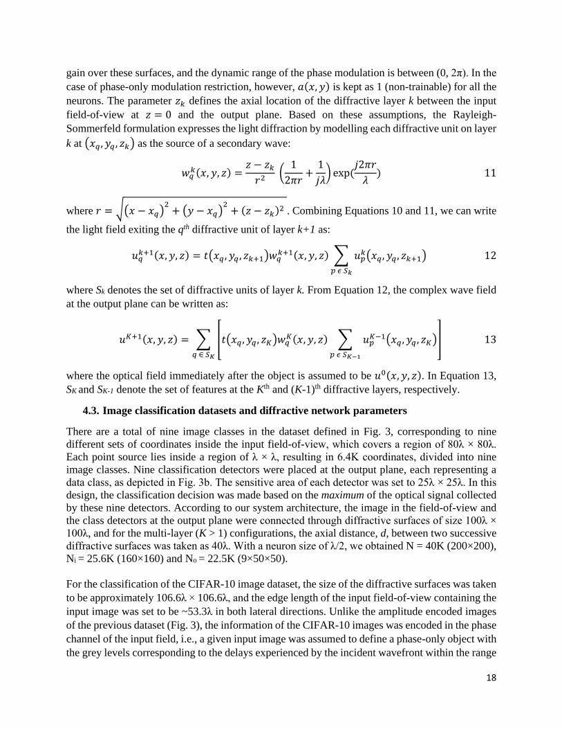
4.2. Optical forward model
In a coherent optical processor composed of diffractive surfaces, the optical transformation
between a given pair of input/output fields-of-view is established through the modulation of light
by a series of diffractive surfaces, which we modelled as two-dimensional, thin, multiplicative
elements. According to our formulation, the complex-valued transmittance of a diffractive surface,
k, is defined as:
𝑡(𝑥, 𝑦, 𝑧𝑘) = 𝑎(𝑥, 𝑦) exp(𝑗2𝜋𝜙(𝑥, 𝑦)) 10
where 𝑎(𝑥, 𝑦) and 𝜙(𝑥, 𝑦) denote the trainable amplitude and the phase modulation functions of
diffractive layer k. The values of 𝑎(𝑥, 𝑦), in general, lie in the interval (0, 1), i.e., there is no optical
𝑛ℎ = 1 +∑1
𝑞1
𝑘=2
+ ∑ 𝑞1
𝑝2+𝑞1
𝑘=𝑞1+1
+ ∑ (𝑝2
𝑞3+𝑝2
𝑘=𝑝2+𝑞1+1
+ 1) + ∑ 𝑞3
𝑝4+𝑞3
𝑘=𝑞3+𝑝2+1
+ ∑ (𝑝4
𝑞5+𝑝4
𝑘=𝑝4+𝑞3+1
+ 1) + ∑ 𝑞5
𝑝6+𝑞5
𝑘=𝑞5+𝑝4+1
+ ∑ (𝑝6
𝑞7+𝑝6
𝑘=𝑝6+𝑞5+1
+ 1)
+ ⋯
+ ∑ (𝑝𝑠−2
𝑁𝐿1+𝑝𝑠−2
𝑘=𝑝s−2+𝑞𝑠−3+1
+ 1) + ∑ 𝑁𝐿1
𝑁𝐿1+𝑁𝐿2−1
𝑘=𝑁𝐿1+𝑝𝑠−2+1
9
18
gain over these surfaces, and the dynamic range of the phase modulation is between (0, 2π). In the
case of phase-only modulation restriction, however, 𝑎(𝑥, 𝑦) is kept as 1 (non-trainable) for all the
neurons. The parameter 𝑧𝑘 defines the axial location of the diffractive layer k between the input
field-of-view at 𝑧 = 0 and the output plane. Based on these assumptions, the Rayleigh-
Sommerfeld formulation expresses the light diffraction by modelling each diffractive unit on layer
k at (𝑥𝑞 , 𝑦𝑞 , 𝑧𝑘) as the source of a secondary wave:
𝑤𝑞𝑘(𝑥, 𝑦, 𝑧) =
𝑧 − 𝑧𝑘𝑟2
(1
2𝜋𝑟+1
𝑗𝜆) exp (
𝑗2𝜋𝑟
𝜆) 11
where 𝑟 = √(𝑥 − 𝑥𝑞)2+ (𝑦 − 𝑥𝑞)
2+ (𝑧 − 𝑧𝑘)
2 . Combining Equations 10 and 11, we can write
the light field exiting the qth diffractive unit of layer k+1 as:
𝑢𝑞𝑘+1(𝑥, 𝑦, 𝑧) = 𝑡(𝑥𝑞 , 𝑦𝑞 , 𝑧𝑘+1)𝑤𝑞
𝑘+1(𝑥, 𝑦, 𝑧) ∑ 𝑢𝑝𝑘(𝑥𝑞, 𝑦𝑞 , 𝑧𝑘+1)
𝑝 𝜖 𝑆𝑘
12
where Sk denotes the set of diffractive units of layer k. From Equation 12, the complex wave field
at the output plane can be written as:
𝑢𝐾+1(𝑥, 𝑦, 𝑧) = ∑ [𝑡(𝑥𝑞 , 𝑦𝑞 , 𝑧𝐾)𝑤𝑞𝐾(𝑥, 𝑦, 𝑧) ∑ 𝑢𝑝
𝐾−1(𝑥𝑞 , 𝑦𝑞 , 𝑧𝐾)
𝑝 𝜖 𝑆𝐾−1
]
𝑞 ∈ 𝑆𝐾
13
where the optical field immediately after the object is assumed to be 𝑢0(𝑥, 𝑦, 𝑧). In Equation 13,
SK and SK-1 denote the set of features at the Kth and (K-1)th diffractive layers, respectively.
4.3. Image classification datasets and diffractive network parameters
There are a total of nine image classes in the dataset defined in Fig. 3, corresponding to nine
different sets of coordinates inside the input field-of-view, which covers a region of 80λ × 80λ.
Each point source lies inside a region of λ × λ, resulting in 6.4K coordinates, divided into nine
image classes. Nine classification detectors were placed at the output plane, each representing a
data class, as depicted in Fig. 3b. The sensitive area of each detector was set to 25λ × 25λ. In this
design, the classification decision was made based on the maximum of the optical signal collected
by these nine detectors. According to our system architecture, the image in the field-of-view and
the class detectors at the output plane were connected through diffractive surfaces of size 100λ ×
100λ, and for the multi-layer (K > 1) configurations, the axial distance, d, between two successive
diffractive surfaces was taken as 40λ. With a neuron size of λ/2, we obtained N = 40K (200×200),
Ni = 25.6K (160×160) and No = 22.5K (9×50×50).
For the classification of the CIFAR-10 image dataset, the size of the diffractive surfaces was taken
to be approximately 106.6λ × 106.6λ, and the edge length of the input field-of-view containing the
input image was set to be ~53.3λ in both lateral directions. Unlike the amplitude encoded images
of the previous dataset (Fig. 3), the information of the CIFAR-10 images was encoded in the phase
channel of the input field, i.e., a given input image was assumed to define a phase-only object with
the grey levels corresponding to the delays experienced by the incident wavefront within the range

19
[0, λ). To form the phase-only object inputs based on the CIFAR-10 dataset, we converted the
RGB samples to greyscale by computing their YCrCb representations. Then, unsigned 8-bit integer
values in the Y channel were converted into float32 values and normalized to the range [0, 1].
These normalized greyscale images were then mapped to phase values between [0, 2π). The
original CIFAR-10 dataset49 has 50K training and 10K test images. In the diffractive optical
network designs presented here, we used all 50K and 10K images during the training and testing
stages, respectively. Therefore, the blind classification accuracy, efficiency and optical signal
contrast values depicted in Fig. 6 were computed over the entire 10K test set. Supplementary
Figures S4 and S5 demonstrate 600 examples of the greyscale CIFAR-10 images used in the
training and testing phases of the presented diffractive network models, respectively.
The responsivity of the 10 class detectors placed at the output plane (each representing one CIFAR-
10 data class, e.g., automobile, ship, truck, etc.) was assumed to be identical and uniform over an
area of 6.4λ × 6.4λ. The axial distance between two successive diffractive surfaces in the design
was assumed to be 40λ. Similarly, the input and output fields-of-view were placed 40λ away from
the first and last diffractive layers, respectively.
4.4. Loss functions and training details
For a given dataset with C classes, one way of designing an all-optical diffractive classification
network is to place C class detectors at the output plane, establishing a one-to-one correspondence
between data classes and the opto-electronic detectors. Accordingly, the training of these systems
aims to find/optimize the diffractive surfaces that can route most of the input photons, thus the
optical signal power, to the corresponding detector representing the data class of a given input
object.
The first loss function that we used for the training of diffractive optical networks is the cross-
entropy loss, which is frequently used in machine learning for multi-class image classification.
This loss function acts on the optical intensities collected by the class detectors at the output plane
and is defined as:
ℒ = −∑ 𝑔𝑐log (ℴ𝑐)
𝑐 𝜖 𝐶
14
where 𝑔𝑐 and ℴ𝑐 denote the entry in the one-hot label vector and the class score of class c,
respectively. The class score ℴ𝑐, on the other hand, is defined as a function of the normalized
optical signals, 𝑰′;
ℴ𝑐 =exp(𝐼𝑐
′)
∑ exp (𝐼𝑐′)𝑐 𝜖 𝐶 15
Equation 15 is the well-known softmax function. The normalized optical signals 𝑰′ are defined as 𝑰
max {𝑰}× 𝑇, where I is the vector of the detected optical signals for each class detector and T is a
constant parameter that induces a virtual contrast, helping to increase the efficacy of training.

20
Alternatively, the all-optical classification design achieved using a diffractive network can be cast
as a coherent image projection problem by defining a ground-truth spatial intensity profile at the
output plane for each data class and an associated loss function that acts over the synthesized
optical signals at the output plane. Accordingly, the mean-squared-error (MSE) loss function used
in Fig. 6 computes the difference between a ground-truth intensity profile, 𝐼𝑔𝑐(𝑥, 𝑦), devised for
class c and the intensity of the complex wave field at the output plane, i.e., |𝑢𝐾+1(𝑥, 𝑦)|2. We
defined 𝐼𝑔𝑐(𝑥, 𝑦) as:
𝐼𝑔𝑐(𝑥, 𝑦) = {
1 𝑖𝑓 𝑥 𝜖 𝐷𝑥𝑐 𝑎𝑛𝑑 𝑦 𝜖 𝐷𝑦
𝑐
0 𝑜𝑡ℎ𝑒𝑟𝑤𝑖𝑠𝑒 16
where 𝐷𝑥𝑐 and 𝐷𝑦
𝑐 represent the sensitive/active area of the class detector corresponding to class c.
The related MSE loss function, ℒ𝑚𝑠𝑒, can then be defined as:
ℒ𝑚𝑠𝑒 = ∫∫||𝑢𝐾+1(𝑥, 𝑦)|2 − 𝐼𝑔
𝑐(𝑥, 𝑦)|2𝑑𝑥𝑑𝑦 17
All network models used in this work were trained using Python (v3.6.5) and TensorFlow (v1.15.0,
Google Inc.). We selected the Adam50 optimizer during the training of all the models, and its
parameters were taken as the default values used in TensorFlow and kept identical in each model.
The learning rate of the diffractive optical networks was set to 0.001.
References
1. Pendry, J. B. Negative Refraction Makes a Perfect Lens. Physical Review Letters 85, 3966–3969
(2000).
2. Cubukcu, E., Aydin, K., Ozbay, E., Foteinopoulo, S. & Soukoulis, C. M. Negative refraction by
photonic crystals. Nature 423, 604–605 (2003).
3. Fang, N. Sub-Diffraction-Limited Optical Imaging with a Silver Superlens. Science 308, 534–537
(2005).
4. Jacob, Z., Alekseyev, L. V. & Narimanov, E. Optical Hyperlens: Far-field imaging beyond the
diffraction limit. 10 (2006).
5. Engheta, N. Circuits with Light at Nanoscales: Optical Nanocircuits Inspired by Metamaterials.
Science 317, 1698–1702 (2017).

21
6. Liu, Z., Lee, H., Xiong, Y., Sun, C. & Zhang, X. Far-Field Optical Hyperlens Magnifying Sub-
Diffraction-Limited Objects. Science 315, 1686–1686 (2007).
7. MacDonald, K. F., Sámson, Z. L., Stockman, M. I. & Zheludev, N. I. Ultrafast active plasmonics.
Nature Photonics 3, 55–58 (2009).
8. Lin, D., Fan, P., Hasman, E. & Brongersma, M. L. Dielectric gradient metasurface optical elements.
Science 345, 298–302 (2014).
9. Yu, N. & Capasso, F. Flat optics with designer metasurfaces. Nature Materials 13, 139–150 (2014).
10. Kuznetsov, A. I., Miroshnichenko, A. E., Brongersma, M. L., Kivshar, Y. S. & Luk’yanchuk, B.
Optically resonant dielectric nanostructures. Science 354, aag2472 (2016).
11. Shalaev, V. M. Optical negative-index metamaterials. Nature Photonics 1, 41–48 (2007).
12. Chen, H.-T., Taylor, A. J. & Yu, N. A review of metasurfaces: physics and applications. Reports on
Progress in Physics 79, 076401 (2016).
13. Smith, D. R. Metamaterials and Negative Refractive Index. Science 305, 788–792 (2004).
14. Yu, N. et al. Flat Optics: Controlling Wavefronts With Optical Antenna Metasurfaces. IEEE Journal
of Selected Topics in Quantum Electronics 19, 4700423–4700423 (2013).
15. Maier, S. A. et al. Local detection of electromagnetic energy transport below the diffraction limit in
metal nanoparticle plasmon waveguides. Nature Materials 2, 229–232 (2003).
16. Alù, A. & Engheta, N. Achieving transparency with plasmonic and metamaterial coatings. Physical
Review E 72, (2005).
17. Schurig, D. et al. Metamaterial Electromagnetic Cloak at Microwave Frequencies. Science 314, 977–
980 (2006).
18. Pendry, J. B. Controlling Electromagnetic Fields. Science 312, 1780–1782 (2006).
19. Cai, W., Chettiar, U. K., Kildishev, A. V. & Shalaev, V. M. Optical cloaking with metamaterials.
Nature Photonics 1, 224–227 (2007).
20. Valentine, J., Li, J., Zentgraf, T., Bartal, G. & Zhang, X. An optical cloak made of dielectrics. Nature
Materials 8, 568–571 (2009).

22
21. Narimanov, E. E. & Kildishev, A. V. Optical black hole: Broadband omnidirectional light absorber.
Applied Physics Letters 95, 041106 (2009).
22. Oulton, R. F. et al. Plasmon lasers at deep subwavelength scale. Nature 461, 629–632 (2009).
23. Zhao, Y., Belkin, M. A. & Alù, A. Twisted optical metamaterials for planarized ultrathin broadband
circular polarizers. Nature Communications 3, (2012).
24. Watts, C. M. et al. Terahertz compressive imaging with metamaterial spatial light modulators. Nature
Photonics 8, 605–609 (2014).
25. Estakhri, N. M., Edwards, B. & Engheta, N. Inverse-designed metastructures that solve equations.
Science 363, 1333–1338 (2019).
26. Hughes, T. W., Williamson, I. A. D., Minkov, M. & Fan, S. Wave physics as an analog recurrent
neural network. Science Advances 5, eaay6946 (2019).
27. Qian, C. et al. Performing optical logic operations by a diffractive neural network. Light: Science &
Applications 9, (2020).
28. Psaltis, D., Brady, D., Gu, X.-G. & Lin, S. Holography in artificial neural networks. Nature 343,
325–330 (1990).
29. Shen, Y. et al. Deep learning with coherent nanophotonic circuits. Nature Photon 11, 441–446
(2017).
30. Shastri, B. J. et al. Neuromorphic Photonics, Principles of. in Encyclopedia of Complexity and
Systems Science (ed. Meyers, R. A.) 1–37 (Springer Berlin Heidelberg, 2018). doi:10.1007/978-3-
642-27737-5_702-1.
31. Bueno, J. et al. Reinforcement learning in a large-scale photonic recurrent neural network. Optica 5,
756 (2018).
32. Feldmann, J., Youngblood, N., Wright, C. D., Bhaskaran, H. & Pernice, W. H. P. All-optical spiking
neurosynaptic networks with self-learning capabilities. Nature 569, 208–214 (2019).
33. Miscuglio, M. et al. All-optical nonlinear activation function for photonic neural networks [Invited].
Optical Materials Express 8, 3851 (2018).

23
34. Tait, A. N. et al. Neuromorphic photonic networks using silicon photonic weight banks. Scientific
Reports 7, (2017).
35. George, J. et al. Electrooptic Nonlinear Activation Functions for Vector Matrix Multiplications in
Optical Neural Networks. in Advanced Photonics 2018 (BGPP, IPR, NP, NOMA, Sensors, Networks,
SPPCom, SOF) SpW4G.3 (OSA, 2018). doi:10.1364/SPPCOM.2018.SpW4G.3.
36. Mehrabian, A., Al-Kabani, Y., Sorger, V. J. & El-Ghazawi, T. PCNNA: A Photonic Convolutional
Neural Network Accelerator. in 2018 31st IEEE International System-on-Chip Conference (SOCC)
169–173 (2018). doi:10.1109/SOCC.2018.8618542.
37. Sande, G. V. der, Brunner, D. & Soriano, M. C. Advances in photonic reservoir computing.
Nanophotonics 6, 561–576 (2017).
38. Lin, X. et al. All-optical machine learning using diffractive deep neural networks. Science 361, 1004–
1008 (2018).
39. Li, J., Mengu, D., Luo, Y., Rivenson, Y. & Ozcan, A. Class-specific differential detection in
diffractive optical neural networks improves inference accuracy. AP 1, 046001 (2019).
40. Mengu, D., Luo, Y., Rivenson, Y. & Ozcan, A. Analysis of Diffractive Optical Neural Networks and
Their Integration With Electronic Neural Networks. IEEE J. Select. Topics Quantum Electron. 26, 1–
14 (2020).
41. Veli, M. et al. Terahertz Pulse Shaping Using Diffractive Legos. arXiv:2006.16599 [cs, physics].
42. Luo, Y. et al. Design of task-specific optical systems using broadband diffractive neural networks.
Light Sci Appl 8, 112 (2019).
43. Mengu, D. et al. Misalignment resilient diffractive optical networks. Nanophotonics 0, (2020).
44. Li, J. et al. Machine Vision using Diffractive Spectral Encoding. arXiv:2005.11387 [cs, eess,
physics] (2020).
45. Esmer, G. B., Uzunov, V., Onural, L., Ozaktas, H. M. & Gotchev, A. Diffraction field computation
from arbitrarily distributed data points in space. Signal Processing: Image Communication 22, 178–
187 (2007).

24
46. Goodman, J. W. Introduction to Fourier Optics. (Roberts and Company Publishers, 2005).
47. Zhang, Z., You, Z. & Chu, D. Fundamentals of phase-only liquid crystal on silicon (LCOS) devices.
Light: Science & Applications 3, e213–e213 (2014).
48. Moon, T. K. & Sterling, W. C. Mathematical Methods and Algorithms for Signal Processing. (2000).
49. CIFAR-10 and CIFAR-100 datasets. https://www.cs.toronto.edu/~kriz/cifar.html.
50. Kingma, D. P. & Ba, J. Adam: A Method for Stochastic Optimization. arXiv:1412.6980 [cs] (2014).

25
Figures and Tables
Fig. 1: Schematic of a multi-surface diffractive network. a Schematic of a diffractive optical network that connects an
input field-of-view (aperture) composed of 𝑁𝑖 points to a desired region-of-interest at the output plane/aperture covering
𝑁𝑜 points, through K diffractive surfaces with N neurons per surface, sampled at a period of 𝜆 2𝑛⁄ , where 𝜆 and 𝑛 represent
the illumination wavelength and the refractive index of the medium between the surfaces, respectively. Without loss of
generality, 𝑛 = 1 was assumed in this manuscript. b The communication between two successive diffractive surfaces occurs
through propagating waves when the axial separation (d) between these layers is larger than 𝜆. Even if the diffractive surface
has deeply sub-wavelength structures, as in the case of, e.g., metasurfaces, with a much smaller sampling period compared
to 𝜆 2⁄ and many more degrees of freedom (M) compared to N, the information processing capability of a diffractive surface
within a network is limited to propagating modes since d ≥ λ; this limits the effective number of neurons per layer to N, even
for a surface with M >> N. H and H* refer to the forward and backward wave propagation, respectively.

26
Fig. 2: Dimensionality (D) of the all-optical solution space covered by multi-layer diffractive networks. a The
behaviour of the dimensionality of the all-optical solution space as the number of layers increases for two different diffractive
surface designs with 𝑁 = 𝑁1 and 𝑁 = 𝑁2 neurons per surface, where 𝑁2 > 𝑁1. The smallest number of diffractive surfaces,
⌈Ks⌉, satisfying the condition 𝐾𝑆𝑁 − (𝐾𝑆 − 1) ≥ 𝑁𝑖 × 𝑁𝑜 determines the ideal depth of the network for a given N, 𝑁𝑖 and
𝑁𝑂. For the sake of simplicity, we assumed 𝑁𝑖 = 𝑁𝑜 = 𝑁𝐹𝑂𝑉−𝑖, where 4 different input/output fields-of-view are illustrated
in the plot, i.e., 𝑁𝐹𝑂𝑉−4 > 𝑁𝐹𝑂𝑉−3 > 𝑁𝐹𝑂𝑉−2 > 𝑁𝐹𝑂𝑉−1. ⌈Ks⌉ refers to the ceiling function, defining the number of diffractive
surfaces within an optical network design. b The distribution of the dimensionality of the all-optical solution space as a
function of N and K for 4 different fields-of-view, 𝑁𝐹𝑂𝑉−𝑖, and the corresponding turning points, Si, which are shown in (a).
For K=1, d1 ≠ d2 is assumed. Also see Supplementary Figures S1-S3 for some examples of K=1, 2 and 3.

27
Fig. 3: Spatially encoded image classification dataset. a Nine image data classes are shown (presented in different
colours), defined inside the input field-of-view (80λ × 80λ). Each λ × λ area inside the field-of-view is randomly assigned
to one image data class. An image belongs to a given data class if and only if all of its nonzero entries belong to the pixels
that are assigned to that particular data class. b The layout of the 9 class detectors positioned at the output plane. Each
detector has an active area of 25λ × 25λ, and for a given input image, the decision on class assignment is made based on the
maximum optical signal among these 9 detectors. c Side view of the schematic of the diffractive network layers, as well as
the input and output fields-of-view. d Example images for 9 different data classes. Three samples for each image data class
are illustrated here, randomly drawn from the 3 test datasets (Te1, Te50, and Te90) that were used to quantify the blind
inference accuracies of our diffractive network models (see Fig. 4).
28
Fig. 4: Training and testing accuracy results for the diffractive surfaces that perform image classification (Figure 3).
a The training and testing classification accuracies achieved by optical network designs composed of diffractive surfaces
that control only the phase of the incoming waves; the training image set is Tr1 (200K images). b The training and testing
classification accuracies achieved by optical network designs composed of diffractive surfaces that can control both the
phase and amplitude of the incoming waves; the training image set is Tr1. c,d Same as in (a,b), respectively, except that the
training image set is Tr2 (6.4K images). N = 40K neurons, and mN = 122.5K neurons, i.e., m>3.
29
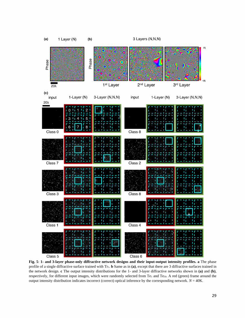
Fig. 5: 1- and 3-layer phase-only diffractive network designs and their input-output intensity profiles. a The phase
profile of a single diffractive surface trained with Tr1. b Same as in (a), except that there are 3 diffractive surfaces trained in
the network design. c The output intensity distributions for the 1- and 3-layer diffractive networks shown in (a) and (b),
respectively, for different input images, which were randomly selected from Te1 and Te50. A red (green) frame around the
output intensity distribution indicates incorrect (correct) optical inference by the corresponding network. N = 40K.

30
Fig. 6: Comparison of the 1-, 3- and 5-layer diffractive networks trained for CIFAR-10 image classification using the
MSE and cross-entropy loss functions. a Results for diffractive surfaces that modulate only the phase information of the
incoming wave. b Results for diffractive surfaces that modulate both the phase and amplitude information of the incoming
wave. The increase in the dimensionality of the all-optical solution space with additional diffractive surfaces of a network
brings significant advantages in terms of generalization, blind testing accuracy, classification efficiency and optical signal
contrast. The classification efficiency denotes the ratio of the optical power detected by the correct class detector with respect
to the total detected optical power by all the class detectors at the output plane. Optical signal contrast refers to the normalized
difference between the optical signals measured by the ground-truth (correct) detector and its strongest competitor detector
at the output plane.

31
Table 1. Coefficient (𝑐𝑘) and basis vector (𝒃𝒌) generation algorithm pseudo-code for an optical
network that has two diffractive surfaces. See the theoretical analysis and Equation 6 of the main
text. See also Supplementary Tables S1-S3.
1 Randomly choose 𝑡1,𝑖 from the set 𝐶1,1 and 𝑡2,𝑗 from the set 𝐶2,1, and assign desired values to
the chosen 𝑡1,𝑖 and 𝑡2,𝑗
2 𝑐1𝒃𝟏 = 𝑡1,𝑖𝑡2,𝑗𝒉𝒊𝒋
3 k=2
4
Randomly choose 𝑻𝟏 or 𝑻𝟐 if 𝐶1,𝑘 ≠ ∅ and 𝐶2,𝑘 ≠ ∅
Choose 𝑻𝟏 if 𝐶1,𝑘 ≠ ∅ and 𝐶2,𝑘 = ∅
Choose 𝑻𝟐 if 𝐶1,𝑘 = ∅ and 𝐶2,𝑘 ≠ ∅
5 If 𝑻𝟏 is chosen in Step 4:
6 Randomly choose 𝑡1,𝑖 from the set 𝐶1,𝑘, and assign a desired value to the chosen 𝑡1,𝑖
7 𝑐𝑘𝒃𝒌 = 𝑡1,𝑖 (∑ 𝑡2,𝑗𝒉𝒊𝒋 𝑡2,𝑗∉𝐶2,𝑘 )
8 else:
9 Randomly choose 𝑡2,𝑗 from the set 𝐶2,𝑘, and assign a desired value to the chosen 𝑡2,𝑗
10 𝑐𝑘𝒃𝒌 = 𝑡2,𝑗(∑ 𝑡1,𝑖𝒉𝒊𝒋 𝑡1,𝑖∉𝐶1,𝑘 )
11 k = k+1
12 If 𝐶1,𝑘 ≠ ∅ or 𝐶2,𝑘 ≠ ∅:
13 Return to Step 4
14 else:
15 Exit